Abstract
630.0 nm all-sky imaging data are used to detect airglow depletions associated with equatorial spread F. Pairs of imagers located at geomagnetically conjugate locations in the American sector at low and mid-latitudes provide information on the occurrence rate and zonal motion of airglow depletions. Airglow depletions are seen extending to magnetic latitudes as high as 25°. An asymmetric extension is observed with structures in the northern hemisphere reaching higher latitudes. By tracking the zonal motion of airglow depletions, zonal plasma drifts in the thermosphere can be inferred and their simultaneous behavior in both hemispheres investigated. Case studies using El Leoncito and Mercedes imagers in the southern hemisphere, and the respective magnetically conjugate imagers at Villa de Leyva and Arecibo, provide consistent evidence of the influence of the South Atlantic Magnetic Anomaly on the dynamics and characteristics of the thermosphere–ionosphere system at low and mid-latitudes.
1. Introduction
The equatorial and low latitude ionospheric region hosts a variety of processes, including the occurrence of ionospheric irregularities, commonly known as equatorial spread F (ESF), as well as the enhancements in the neutral temperature near the local midnight—the midnight temperature maximum (MTM). The crests of the equatorial ionization anomaly (EIA), typically located between 10° and 20° magnetic latitude, depending among other factors on solar activity, can be used to define the boundaries of the low latitude region. Poleward from the crests, other processes are observed, like medium-scale travelling ionospheric disturbances (MSTIDs). One then can expect the region between ~15° and 25° magnetic latitude to be a transition zone from the dominance of equatorial to mid-latitude physics.
All-sky imagers (ASIs) are optical instruments that provide information about these processes by measuring airglow emissions at different wavelengths. When looking at the 630.0 nm emission, the result of the dissociative recombination of O2+, followed by the relaxation of the excited atomic oxygen state O (1D), an all-sky imaging system can sample an area of ~106 km2 at 250 km, and thus one can measure these processes when they do not occur directly overhead. For example, from an instrument located at ~20° geographic latitude, like the one at the Arecibo Observatory, structures seen in 630.0 nm to the south at a ~75° zenith angle are occurring at ~10° geographic latitude, very close to the region where the northern crest of the EIA can be found.
Boston University has established a network of ASIs with sites at opposite ends of the same geomagnetic field lines in each hemisphere, i.e., geomagnetic conjugate sites [1]. The ASIs are autonomous instruments that operate in mini-observatories situated at four conjugate pairs in North and South America, plus one pair linking Europe and South Africa. In this paper, we describe results from two pairs of ASIs in the American longitude sector, Arecibo (18.3° N, 66.7° W) and Mercedes (34.7° S, 59.4° W), and El Leoncito (31.8° S, 69.3° W) and Villa de Leyva (5.6° N, 73.5° W). Raw images need to be processed in order to assign a latitude and longitude to every pixel. This implies that an emission height needs to be assumed, and during low solar activity, 250 km is typically used. For a more quantitative way to determine the emission altitude, the Boston University Airglow Model [2] is used. In this model the airglow emission altitude is calculated using ionospheric profiles from IRI-2016 [3] and thermospheric profiles from NRLMSISE-00 [4].
Figure 1 shows a map with the fields of view of the imagers, assuming an emission height of 250 km and zenith angles less than 80°. The dashed lines represent apex height contours of 750 and 2400 km, corresponding to magnetic latitudes of 15° and 30°, respectively. During low solar activity, the common feature observed at these sites is the wave-like pattern of medium-scale travelling ionospheric disturbances (MSTIDs). During mid and high solar activity, ESF structures tend to be more common, with some reaching apex heights (height of a magnetic field line at the geomagnetic equator) as high as ~2000 km. Thus, in addition to seeing ESF signatures frequently at El Leoncito and Villa de Leyva, the “low latitude sites”, close to ~15° magnetic latitude, they can also be detected at Mercedes and Arecibo, the “mid-latitude sites”, close to ~25° magnetic latitude. The zenith locations of the Mercedes and Arecibo ASIs are poleward from the crests of the equatorial ionization anomaly and the processes typically observed at the equatorial and low-latitude sites (like ESF) do not frequently reach zenith.
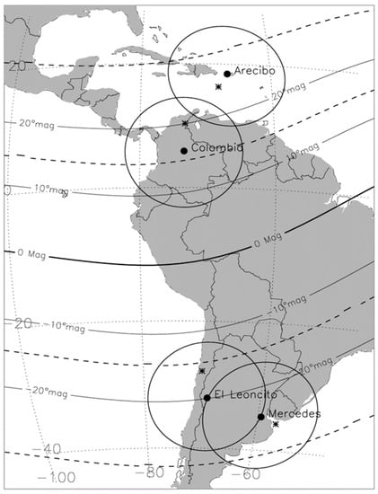
Figure 1.
Map showing the locations and fields of view of the all-sky imagers used in this study. Circles represent the FOV at 250 km and zenith angles less than 80°. The black dots refer to the zenith at each location and asterisks identify the magnetically conjugate imager’s zenith. The magnetic equator and ±10° and ±20° magnetic latitude lines are indicated. The dashed curves represent the apex heights of 750 km and 2400 km.
The work by [5] showed examples of airglow depletions reaching the field of view of the Arecibo all-sky imager that were associated with equatorial spread F. A case shown in that study used the El Leoncito ASI, in the southern hemisphere, with a field of view overlapping with a small region of the mapped Arecibo ASI, and detected a depletion that was also observed in the Arecibo ASI. This was evidence of the geomagnetically conjugate behavior of the structures associated with ESF; but, as stated above, ESF-related airglow depletions are not very common at the Arecibo latitudes. Reference [6] analyzed the occurrence rate of MSTIDs, a more common phenomenon at these latitudes, during the 2002–2007 period and showed that peaks of ~60% were observed during the winter and summer solstices. The unusually high winter peak, not observed at other longitude sectors [7], prompted speculation on the influence of the opposite hemisphere on the formation of MSTIDs. Driven by these previous studies, an all-sky imager was installed at Mercedes, near the conjugate point of Arecibo. As a result, reference [8] showed simultaneous and conjugate observations of MSTIDs at the two sites and proposed that the particular conditions in this longitude sector in the southern hemisphere, like the presence of the South Atlantic Magnetic Anomaly and a high occurrence of sporadic E layer structures, were responsible for the patterns observed.
This study will investigate the occurrence of ESF-related airglow depletions at Arecibo and will compare magnetically conjugate observations using the imagers at Arecibo and Mercedes and, to the west, at El Leoncito and Villa de Leyva.
2. Observations
2.1. Arecibo ESF Depletions
ESF-related structures are not common at latitudes above ~20° magnetic latitude. Reference [6] studied the seasonal behavior of MSTIDs using the Arecibo ASI during the years 2002–2007. They showed peak occurrence rates close to 60% during both solstices. Figure 2 shows the percentage occurrence rate of the ESF-related structures at Arecibo during the same period. The occurrence rate is much smaller (~15%) and peaks during the December solstice. This result is in agreement with the general longitudinal morphology of ESF occurrence at low latitudes [9,10,11].
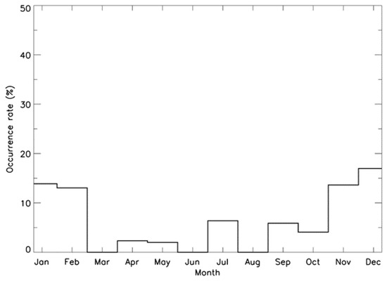
Figure 2.
Seasonal variation in the occurrence rate of equatorial spread F (ESF) structures observed inside the field of view of the Arecibo all-sky imager during the 2002–2007 period. A main peak is clearly observed during the December solstice.
The small occurrence rate percentage of ESF-related airglow depletions should not be surprising considering that in order to detect them using 630.0 nm emissions the flux tubes affected (the airglow depletions represent the footpoints of the depleted flux tubes) need to reach magnetic field apex altitudes higher than ~1500 km. This requires, among other factors, strong upward drifts during the post-sunset period. The observations presented here were carried out during the declining phase and minimum phase of solar cycle 23, when upward drifts are small. For the cases observed, a strong correlation with geomagnetic activity was found. Out of the 36 cases of nights with ESF-related airglow depletions, almost 40% occurred during relatively high magnetic activity, when the large rate of change of the equatorial Dst index was close to local sunset. This points to the influence of prompt penetration electric fields that provide an additional source of upward plasma drifts. This effect was discussed in reference [12] when trying to explain the positive or negative effects of a geomagnetic storm in the triggering of ESF. Thus, even if solar activity is not high, ESF effects can be observed at mid-latitudes at locations where, typically, equatorial effects do not reach.
2.2. Magnetically Conjugate Observations
The results described in the previous section prompted subsequent studies involving the ASI installed at the Mercedes Astronomical Observatory in 2009, close to the geomagnetic conjugate point of Arecibo. The next set of results was obtained from May 2009 until February 2012 with the ASIs at Arecibo and Mercedes. This period covers the deepest solar minimum of solar cycle 23 that lasted until early 2010 and the increasing activity of the next cycle. As stated above, in order to observe airglow depletion associated with ESF at high latitudes, particular conditions need to occur, like, high solar activity and/or the proper timing of intensification of geomagnetic storms in the dusk sector to allow the prompt penetration of electric fields to trigger the irregularities [12]. A magnetic field line reaching Mercedes’ zenith (~34o S) at ~250 km has an apex height of ~1800 km. In the northern hemisphere, the same field line reaches ~13° N, i.e., south of Arecibo’s zenith (see Figure 2). Thus, the ASIs at Mercedes and Arecibo allow us to simultaneously study the footpoints of the depleted flux tubes associated with the ESF structures. Figure 3 shows an example of the simultaneous observations of ESF-related airglow depletions on the night of 25 October 2011 at three different times. Three snapshots show a one-to-one correlation between the structures observed at both sites. These images are unwarped at 250 km, and the rest of the analysis using the Mercedes and Arecibo data was also done using 250 km.
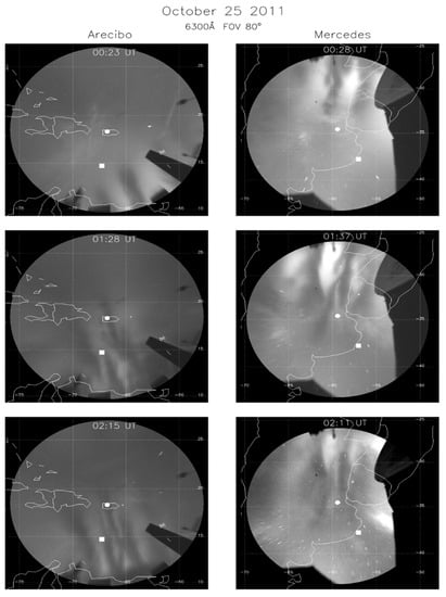
Figure 3.
Simultaneous conjugate observations during 25 October 2011 from Arecibo (left) and Mercedes (right). Images at three different times show a one-to-one correlation between the structures observed at both sites. Images at both sites are unwarped using an altitude of 250 km. Depletions at Mercedes are wider and some of them do not reach latitudes as high as the ones over Arecibo. For example, the middle and bottom panels show a depletion that reaches a ~20° N passing through zenith in the Arecibo imager; but, it is not as clear in the Mercedes imager, hardly reaching the conjugate point, indicated as a white square.
Depletions at Mercedes seem to be wider and some of them seem not to reach similar magnetic latitudes as observed in Arecibo. For example, the middle and bottom panel show a depletion that reaches ~20° S, passing through zenith in the Arecibo imager; however, it is not as clear in the Mercedes imager, hardly reaching the conjugate point, indicated as a white square. Overall, the conjugate images show an excellent spatial correspondence, although some particularities are observed: the longitudinal extent of the depletions seems to be wider in the southern hemisphere, and the latitudinal extension is higher in the northern hemisphere.
Table 1 shows a summary of the number of ESF cases observed from May 2009 to February 2012 and the corresponding average F10.7 index. It is clear that the increased solar activity led to an increase in the number of nights with ESF structures observed at both sites. During the year 2011, not only the number of ESF-related structures increased, but also how far in latitude these structures reached, with some cases extending past the location of Arecibo’s zenith, i.e., apex heights greater than 2400 km (see Figure 1). The number of ESF-related airglow depletions was 81 for Arecibo and 122 for Mercedes. Simultaneous conjugate observations were observed in 51 nights. Due to the lower magnetic latitude of the Mercedes Observatory, more depletions are observed at this site. The simultaneous cases were observed mostly during the December solstice, and, on average, they reached apex heights around 2000 km, so they were visible only to the south of Arecibo and close to zenith at Mercedes.

Table 1.
Summary of the number of ESF-related airglow depletions observed at Mercedes and Arecibo.
Figure 4 shows the occurrence rate of the airglow depletions observed at Arecibo (solid lines) and Mercedes (dashed lines). Both locations show peak occurrence during the December solstice. The higher magnetic latitude of Arecibo explains why the ESF cases are less frequently observed than at Mercedes. The Arecibo result is consistent with the one carried out during the 2002–2007 period (Figure 2), with a higher peak as a consequence of the higher solar activity.
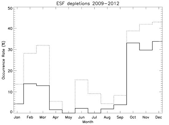
Figure 4.
Occurrence rate of ESF depletions observed at Mercedes (dashed lines) and Arecibo (solid lines). Similar seasonal dependence is observed at both sites, with peak occurrence during the December solstice.
Not all the cases observed during the June solstice occurred during high geomagnetic activity. The main conclusion from the Arecibo–Mercedes simultaneous measurements is that the conjugate behavior of the ESF-related airglow depletions is always observed at these mid-latitude sites, with structures showing very strong similarities in morphology and characteristics; however, we have found cases when the large-scale ESF structures are not symmetric, meaning that they are not observed at similar magnetic latitudes, in particular when they have apex heights higher than ~2000 km. In general, this is observed during solstice conditions when very different background conditions exist at both hemispheres (winter vs. summer) and the contrast between the background and the ESF structure might be affected by them, impacting the detectability of the depletions. Different meridional winds might also affect the plasma distribution, adding another factor that needs to be taken into account when studying the inter-hemispheric characteristics of the airglow depletions associated with ESF.
We also analyzed conjugate observations from the El Leoncito–Villa de Leyva pair, located in the western part of South America, at lower latitudes. A study by [13] combined data from three BU all-sky imagers located in the western part of South America, Villa de Leyva, Jicamarca, and El Leoncito. They investigated the conditions at Jicamarca that would lead to the development of the high altitude, or topside, plumes observed at both hemispheres. Now we use the El Leoncito–Villa de Leyva pair to show that similar structuring is observed in general, although cases were found when the northern hemisphere depletions reach further in latitude. Figure 5 shows an example of conjugate ESF depletions. The left panel shows an unwarped image at Villa de Leyva on 10 March 2015 at 02:06 UT. The BU Airglow Model was used to determine an emission height of 250 km at this time for the two sites. The right panel corresponds to an image from the El Leoncito all-sky imager at the same time. Two depletions with very similar structuring are seen reaching the same magnetic latitudes in both hemispheres.
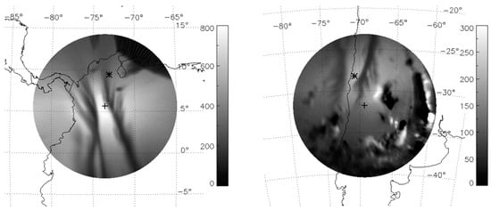
Figure 5.
(left) Unwarped 6300 Å image from the Villa de Leyva ASI at 02:06 UT on 10 March 2015. The cross is the location of the ASI and the asterisk represents the magnetic conjugate location of El Leoncito’s zenith; (right) unwarped simultaneous 6300 Å image from El Leoncito ASI. The asterisk shows the magnetic conjugate location of the northern hemisphere imager’s zenith. Both images were unwarped at 250 km.
Figure 6 shows a more detailed comparison of the structures observed with images covering an area of 5° latitude × 5° longitude. The left image is a zoomed-in region of the Villa de Leyva all-sky image shown in Figure 5. The right image is a zoomed-in region of the mapped El Leoncito image, shown in Figure 5, into the Northern hemisphere using a realistic geomagnetic field model. A remarkable one-to-one correspondence is observed.
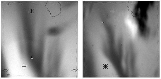
Figure 6.
(left) 5° × 5° zoomed in region close to the zenith of the Villa de Leyva ASI, indicated as a plus symbol. The asterisk represents the conjugate location of El Leoncito’s zenith; (right) 5° × 5° zoomed in mapped region from El Leoncito ASI. The asterisk here represents the conjugate point of Villa de Leyva’s zenith and the plus symbol the location of El Leoncito’s zenith.
But, as it was the case for the Arecibo–Mercedes pair, there are nights when differences are observed, with depletions in one hemisphere reaching higher magnetic latitudes than the ones observed in the opposite hemisphere. An example of such a case is shown in Figure 7. During the night of 29 November 2014, multiple depletions were observed at both sites. Partly cloudy conditions during the night made it difficult to identify the conjugate depletions at all the times. In the same format as Figure 4, Figure 5 and Figure 6, the left panel in Figure 7 shows the unwarped images from the Villa de Leyva all-sky imager at 03:36 UT and 04:13 UT, assuming a 250 km emission height. Apex height contour lines at 500, 700, 900, and 1100 km are shown in black. As the night progresses, the depletions drift to the east. Three depletions that can be observed in multiple images are identified with the letters A, B, and C at Villa de Leyva. The bright wide structure between ~0° and 5° is the northern crest of the equatorial ionization anomaly. The simultaneous images from El Leoncito (right panel) shows conjugate depletions labelled A* and B*. Depletion C* is not observed, even though at Villa de Leyva depletion C is almost reaching an apex height of 700 km. Depletion B* extends from the top of the image to less than the 1100 km apex height, while in the northern hemisphere, depletion B is seen easily reaching 1100 km. The southern crest of the EIA is observed but covering only the eastern part of the field of view.
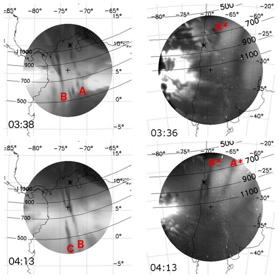
Figure 7.
(left) Villa de Leyva unwarped images at 03:38 UT (top) and 04:13UT (bottom) using an emission height of 250 km. Eastward moving depletions labelled A, B, and C are indicated; (right) simultaneous images from El Leoncito, unwarped at 300 km, where the conjugate depletions are marked as A* and B*. While depletion C extends to almost 700 km apex height, depletion C* is not seen in the field of view of the El Leoncito imager.
In summary, the two pairs of conjugate all-sky imagers have shown that airglow depletions in the southern hemisphere show different characteristics than the ones observed in the northern hemisphere.
2.3. Magnetically Conjugate Zonal Velocities
In addition to the morphological studies of airglow depletions at magnetically conjugate locations, we have also compared the zonal drifts of the depletions obtained by following their motion in both hemispheres. The 630.0 nm all-sky images have been used extensively in the past to determine zonal plasma motion [14,15,16,17]. The zonal velocities of the ESF were taken at various magnetic latitudes along the structure. The velocities were found from a longitude vs. time plot (velogram), which allowed for a quadratic curve to be fit to the zonal motion of the ESF. The derivative of this fit is the zonal velocity. Depletions can also be tracked through multiple images by determining their centers and following their motion. There are two main sources of error in the determination of the velocity. The first source of error is due to emission altitude. For a given image, the higher the height assumed to unwarp it, the larger the velocity. This is because the same image is projected onto a larger area and the distance the depletion travels between the two images will increase. An uncertainty of ±25 km is assumed in the calculation. The second source of error is associated with the determination of the center of the depletion and how this center is tracked at different times. The center of the depletion can be determined within ±10 km, providing a negligible uncertainty in the velocity determination. Overall, a systematic error in the velocity determination of ±20 m/s is obtained. Figure 8 shows an example of the simultaneous velocities obtained from the Arecibo–Mercedes pair at different latitudes, assuming an emission height of 250 km at both sites. Cuts were made at Arecibo at 7° N, 9.5° N, and 12° N, and at Mercedes, in the southern hemisphere, at the respective magnetic conjugate locations: 27° S, 29.5° S, and 32° N. The zonal velocities were computed taking into account the magnetic declination at the location where the depletion is observed. This is important in particular for the Arecibo–Mercedes pair because in this longitude sector magnetic declination can be as high as 20° E. Consistent higher zonal velocities are measured at Mercedes, with a clear latitudinal dependence observed, with lower values at higher latitudes. This has been reported in the past [14] and is the source of the typical inverted C-shape of airglow depletions [18].
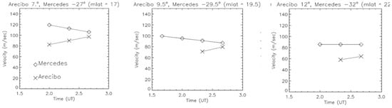
Figure 8.
Example of velocities obtained on 27 February 2011 for depletions at different latitudes: 17° magnetic latitude (left), 19.5° magnetic latitude (center), and 22° magnetic latitude (right). Mercedes values are consistently higher than the ones measured at Arecibo.
In this study we have computed velocities from several nights and multiple depletions. Figure 9 shows the result of combining data from eight quiet nights during the years 2011 and 2012 with 42 individual airglow depletions visible simultaneously at Arecibo and Mercedes. Values are binned every 30 min and each data point is labelled with the initial letter of the site and a number indicating the number of data points used to obtain the average result. It is important to note that in this calculation we are not concerned with latitudinal variations in the velocity, but how the values in one hemisphere compare with the values in the opposite hemisphere. An overall trend of higher speeds in the southern hemisphere is observed, with values being ~30–35% higher.
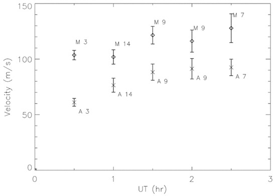
Figure 9.
Zonal velocities from conjugate locations at Arecibo and Mercedes. Each individual data point is computed by averaging the values at different latitudes and binning the data in 30 min intervals. Mercedes values are shown with diamond symbols and Arecibo values with crosses. Each value has a number indicating how many points were used to compute it. Error bars represent the standard deviation of the mean.
Data from the other pair of conjugate sites, Villa de Leyva and El Leoncito, located at lower latitudes, has also been used to investigate the zonal velocities of airglow plasma depletions at both hemispheres. Figure 10 shows three examples on the nights of 12 January 2015 (left), 10 March 2015 (center), and 13 September 2015 (right). Velocities from Villa de Leyva are shown with diamond symbols and velocities from El Leoncito with cross symbols. Vertical bars show the error in the determination of the velocity. Each night shows that the velocities at El Leoncito are consistently higher than those at Villa de Leyva, similar to the result shown in Figure 9, where the southern hemisphere site values are higher.
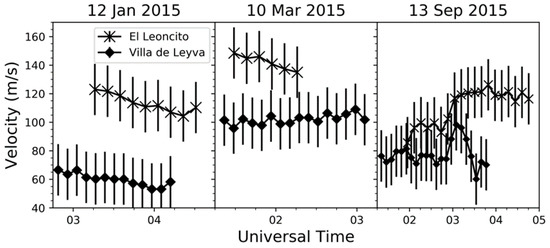
Figure 10.
Zonal velocities calculated on three different nights at Villa de Leyva (diamond) and El Leoncito (cross). Heights used for El Leoncito (Villa de Leyva) were 300, 250, and 260 km (240, 230, and 250 km) for 12 January 2015, 10 March 2015, and 13 September 2015, respectively. Higher zonal drifts are measured in the southern hemisphere.
3. Discussion
Different characteristics of ESF-related airglow depletions have been investigated: the seasonal occurrence of conjugate ESF depletions and the latitudinal extent and zonal velocity of depletions observed simultaneously in both hemispheres. ESF effects are observed at magnetic latitudes as high as ~25°. Previous case studies of conjugate ESF signatures using all-sky imagers showed an exact one-to-one correlation in the latitudinal extent at both hemispheres [19,20]. We have observed depletions in the northern hemisphere that extend to higher latitudes than the corresponding conjugate depletions in the southern hemisphere.
Extreme cases with depleted structures observed in GPS-TEC and airglow data were reported recently [21,22,23]. These structures were associated with ESF and reached magnetic latitudes as high as 40°. Very active geomagnetic conditions were present during these observations. In this work, we show that airglow depletions can reach latitudes that usually are considered outside the region of influence of equatorial processes. Even though the percentage rates are low, as shown in Figure 2 and Figure 4, the detection at mid latitudes of a process—typically constrained to occur at low latitudes—reflects the dynamical coupling between the equatorial and mid-latitude regions. Modeling efforts have not been successful in reproducing ESF-structures reaching apex heights higher than 1500–2000 km. While semi-empirical modeling offered a buoyancy mechanism to account for the >1000 km apex height plumes [24], subsequent full 3D numerical modeling did not achieve similar results [25,26].
In order to determine in a more quantitative way the latitudinal extent of the ESF-related airglow depletions, images from the Villa de Leyva–El Leoncito pair are calibrated to get airglow brightness in Rayleigh units (1 R = 106 photons/cm2secstr) and horizontal cuts are taken through a Villa de Leyva image on 10 March 2015 at two fixed geographic latitudes, 7° and 9°, indicated in Figure 11 (left) as the red horizontal lines. The conjugate locations for every point along the lines have been computed using the IGRF-12 magnetic field model [27] to create the red curves at El Leoncito (right).
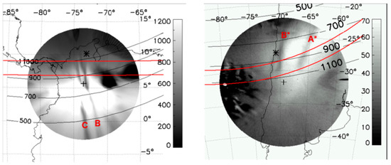
Figure 11.
(left) A 630.0 nm image taken with the Villa de Leyva ASI at 04:13 UT on 29 November 2014. The red lines represent cuts through the image at a constant geographic latitude of 9° N and 7° N. The red letters mark the different depletions. The bright airglow between ~0 and 5° is the northern crest of the equatorial ionization anomaly; (right) simultaneous image from the El Leoncito ASI. The red curves are the conjugate locations of the cuts in the Villa de Leyva image. Solid black contours are lines of constant magnetic apex altitude in kilometers. The gray scale associated with each image shows the emission in Rayleighs. Depletions B and B* are conjugate structures.
At this time the only common depletions observed are labelled B and B*. Depletion B bifurcates into two structures right above zenith in the Villa de Leyva image. We compared the brightness of the two branches of this depletion. Peak airglow at Villa de Leyva is around 1 kR near zenith due to the presence of a very strong northern crest of the EIA. El Leoncito airglow emission is much lower, peaking only at about 70 R. The two conjugate cuts plotted over El Leoncito show that although the depletions reach over 1100 km at Villa de Leyva they do not extend that far in the southern hemisphere. Figure 12 shows the brightness values along the fixed latitudes on the Villa de Leyva ASI (blue line). The values for El Leoncito are shown in orange and are mapped along magnetic field lines back to the northern hemisphere in order to display them in the same coordinates as Villa de Leyva.
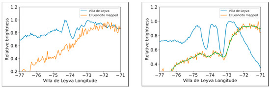
Figure 12.
(left) Blue line represents the normalized brightness obtained from the cut at 9° N over the Villa de Leyva imager. The orange line is the brightness from the conjugate line at El Leoncito (the top red curve on the right image from Figure 11) mapped along magnetic field lines to the Villa de Leyva coordinate system; (right) Normalized brightness from the 7° N cut over Villa de Leyva (blue line). The orange line is the brightness from the conjugate line at El Leoncito (the bottom red curve on the right image from Figure 11). The green line is a running average of 7 pixels to make the depletions more clearly visible. Only the right panel shows that two depletions are visible at Villa de Leyva and El Leoncito between −73° and −75° longitudes.
The data has been normalized to the maximum value along the lines. The left plot corresponds to the 9° N cut, showing no depleted airglow in the El Leoncito data, while the right plot, corresponding to the 7° N cut, shows very clearly the depletions at Villa de Leyva and El Leoncito (an average curve, in green, was overlaid to help identify the two depletions observed at El Leoncito).
We next explore the potential reasons for the different latitude reach: height chosen to unwarp the images, observational limitations due to weak airglow, and different background conditions due to meridional winds. The altitude of the airglow emission could contribute to the different latitudinal extent of the depletions. Recently, reference [2] showed how variations in the assumed airglow emission altitude can lead to apparent interhemispheric asymmetries in the of ESF depletions, in particular when looking at the tilt of the depletions. For the cases presented in Figure 3 and Figure 7, in order to have the depletions reaching the same apex heights in both hemispheres, the images from the southern hemisphere sites would have to be unwarped ~200 km higher than the heights used in the analysis, an unrealistic situation because this would imply a peak emission height close to 500 km. Changes in the 630.0 nm airglow emission can be a result of changes in electron density or changes in the height of the F layer. Another wavelength used in all-sky imagers is 777.4 nm, sensitive only to changes in total electron content (TEC). In this study, similar results are observed in the 777.4 nm depletions, proving that the lower extent of the El Leoncito depletions is not due to limitations in detectability at 630.0 nm. While the low levels of airglow emission at El Leoncito are not affecting the detectability of the latitudinal extent of the depletions, the difference in brightness between the two sites may offer some insight into why the depletions extent is different. A difference in the background emission at two conjugate sites is a regular occurrence. The gray color scale next to each image in Figure 11 shows that on 29 November 2014 the background 630.0 nm emission is greater at Villa de Leyva than at El Leoncito by a factor of about 15. Using the Boston University airglow model [2] with NRLMSISE-00 and IRI-2016 as inputs, the brightness computed over El Leoncito was 70 R and over Villa de Leyva it was 170 R, only a factor of ~2.5 higher. In order to further investigate the large asymmetry observed in the brightness we looked at the total electron content (TEC) from GPS receivers. At El Leoncito, 20 TECu (1 TECu = 1016 el/m2) was measured at 04:00 UT and over Bogota, a station close to Villa de Leyva, a value of 80 TECu was measured. These measured TEC values can be compared with the TEC outputs from IRI-2016: 19 TECu over El Leoncito, close to the measured value, and 12 TECu over Bogota, ~6.5 times smaller than the measured value. The ratio of measured and modeled TEC over Bogota is similar to the ratio of measured and modeled emission (~7) and thus it accounts for most of the discrepancy between the modeled emission (170 R) and the measured emission (1.2 kR). Plasma redistribution is occurring and this is related to meridional neutral winds that have been previously shown to impact plasma distribution at equatorial and low latitudes [28]. A trans-equatorial wind blowing from the summer hemisphere to the winter hemisphere drags the ions due to ion-neutral collisions and the presence of the magnetic field forces them to move up first and, after they cross the magnetic equator, down along the magnetic field lines, producing an enhancement in TEC and, consequently, in the 630-nm airglow intensity. Meridional winds that are in the same direction in both hemispheres have been shown to modify the equatorial plasma distribution [25]. Average results from Horizontal Wind Model 14 (HWM-14) [29] show that during the December solstice a strong northward wind is present during the night. Specific runs confirm these results, with meridional winds close to 100 m/s at El Leoncito and around 30 m/s at Villa de Leyva. Therefore, northward winds in both hemispheres are likely the major cause of the differences in airglow brightness, TEC, and the latitudinal extent of the airglow depletions.
The second topic studied here included the zonal plasma velocities at conjugate locations in both hemispheres. Several cases using the Arecibo–Mercedes pair have consistently shown the southern hemisphere values larger than the northern hemisphere ones. In addition, case studies using the Villa de Leyva–El Leoncito pair, located closer to the magnetic equator, also show higher velocities in the Southern hemisphere. During the COPEX (Conjugate Point Equatorial Experiment) campaign, conjugate imagers in the Brazilian region at ~ ±10° magnetic latitude were used to compare the characteristics of the conjugate airglow depletions and the conjugate zonal velocities [15,20]. The campaign included GPS receivers that were used to obtain the drifts by measuring how scintillation patterns moved at each location. The main results indicated that there was a perfect symmetry between the depletions observed at both hemispheres. When comparing the zonal drifts inferred from the motion of airglow depletions, they found that they were very similar. These results are different to the ones obtained here.
Model calculations shown in [30] can be used to explain the observations presented in this paper. Using Quasi Dipolar coordinates (a non-orthogonal system that defines magnetic latitudes and longitudes such that they are constant along field lines) and the IGRF-12 magnetic field model, the zonal plasma velocity v is calculated from v = E × B/B2, where E is the electric field and B is the Earth’s magnetic field. The electric field is mainly due to the F-region dynamo given by the following equation: E = −U × B, where U is the Pedersen conductivity-weighted neutral zonal wind and B is the Earth’s magnetic field. These equations can be used to determine the ratio of the velocities at the two sites. The magnetic field is easily calculated at both sites. The electric field requires a more complex analysis, as discussed in [30] where the authors set up a system of basis vectors that are used to map the electric field along magnetic field lines. Mapping electric fields in a QD coordinate system allows for velocities to be mapped along field lines as well using the equation defining v. In their paper they show that the drift velocity can be separated into two components, magnetic zonal and magnetic meridional, both constant along magnetic field lines, by using their basis vectors. Using this technique, they create a map showing the difference in magnetic east and magnetic north velocities between conjugate locations, meaning that it is possible to compute, for example, how much the eastward component varies when it is mapped into the conjugate hemisphere. This is shown in Figure 13 where the map for the zonal component is reproduced. For a purely dipolar geomagnetic field on a spherical Earth all the values in Figure 13 would be 1. Values greater than these idealized dipolar values are plotted with red contours, while values less than the dipolar values are plotted with blue contours. If we consider a horizontal 100 m/s ExB velocity toward magnetic east at magnetic coordinates 30° N, 0° E, 250 km altitude, its horizontal component at the conjugate point is about 145 m/s (reading a scale factor of about 1.45 at the southern conjugate point). If we start with a 100 m/s horizontal magnetic eastward ExB velocity at magnetic coordinates 30° S, 0° E, we see that the velocity in the conjugate hemisphere is about 70 m/s magnetic eastward. These are the deviations from a purely dipolar mapping. This is the result of assuming that the electric potential along a field line is constant, so the potential difference between the two adjacent field lines in the zonal direction is also constant along a magnetic field line. The electric field (or negative of the gradient of the electric potential) and the magnetic field are geometry dependent, so we can conclude that the ExB velocity in one hemisphere has a different magnitude and direction than the velocity at the conjugate location. The contour lines show that zonal velocities near El Leoncito and Mercedes are on average about 1.3–1.4 times greater than the velocities at their conjugate locations. If the Earth’s magnetic field were a pure dipole then the model would show no difference in velocity. This ratio of velocities is consistent with our results, i.e., higher velocities in the Southern hemisphere.
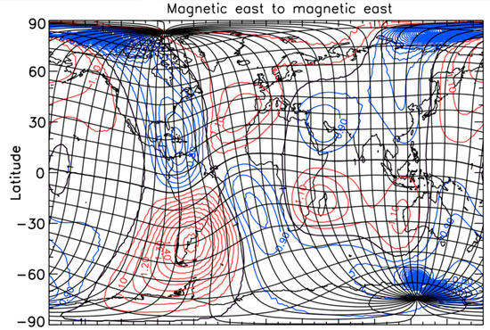
Figure 13.
Map of the zonal velocity differences between conjugate locations. Represented here are the deviations from a purely dipolar mapping. Values greater than these idealized dipolar values are plotted with red contours, while values less than the dipolar values are plotted with blue contours (adapted from [30]).
4. Conclusions
Using all-sky imagers at magnetically conjugate locations, different characteristics of airglow depletions associated with equatorial spread F were investigated. We found that the occurrence of ESF-related airglow depletions at the Arecibo Observatory is more frequent than previously thought. We also investigated the simultaneous occurrence of depletions in both hemispheres and found that during relatively low solar activity they can reach magnetic latitudes as high as 25°. Analysis of the latitudinal extent observed with the two pairs of magnetically conjugate sites shows that the depletions extend to higher latitudes in the northern hemisphere. Background conditions are affected by seasonal differences, but the presence of a net northward wind re-distributes the plasma and affects the way that the depletions behave, causing an inter-hemisphere difference.
We have also investigated the zonal motion of the depletions in both hemispheres. Results show that higher drifts are consistently measured in the Southern hemisphere. On average, the difference is around 30–35%. The faster velocities are attributed to the particular configuration of the magnetic field of the Earth in this longitude sector, i.e., South Atlantic Magnetic Anomaly. Model results indicate that a 100 m/s drift in the northern hemisphere in the American and Caribbean sectors at around 20–25° magnetic latitude is converted into a 130–140 m/s when compared to the drift at the conjugate location. A weaker magnetic field in this region means that there is a smaller zonal ExB drift. The difference in the magnetic field is consistent with the difference in the measured velocity.
Performing magnetically conjugate measurements of airglow depletions associated with ESF provides insights into their characteristics and can help to understand how the Earth’s magnetic field affects the dynamics of ionospheric plasma.
Author Contributions
Conceptualization, C.M. and D.H.; data curation, J.W. and S.P.; investigation, C.M., D.H., C.S., R.M., and J.B.; methodology, C.M., J.B. and J.W.; resources, S.P.; software, J.W.; supervision, C.M.; visualization, C.M., J.W., C.S., D.H. and R.M.; writing—original draft, C.M.; writing—review and editing, C.M., J.W., and D.H. All authors have read and agreed to the published version of the manuscript.
Funding
This work was supported by NSF Aeronomy grant number 1552301, C. Martinis PI. Maintenance and archiving of the all-sky images used in this study are supported by NSF Aeronomy grant number 1659304, M. Mendillo PI. Some of this research was performed while D. Hickey held an NRC Research Associateship award at the US Naval Research Laboratory. D. Hickey’s work is supported by the United States Chief of Naval Research (US CNR).
Acknowledgments
We thank the continuous help of the personnel from the all-sky imager sites used in this study. TEC-GPS values for Bogota and El Leoncito stations were obtained from the LISN website (http://lisn.igp.gob.pe/). All-sky images are available for public viewing as quick-look images and movies at www.buimaging.com.
Conflicts of Interest
The authors declare no conflict of interest.
References
- Martinis, C.; Baumgardner, J.; Wroten, J.; Mendillo, M. All-sky-imaging capabilities for ionospheric space weather research using geomagnetic conjugate point observing sites. Adv. Space Res. 2018, 61, 1636–1651. [Google Scholar] [CrossRef]
- Hickey, D.A.; Sau, S.; Narayanan, V.L.; Gurubaran, S. A possible explanation of interhemispheric asymmetry of equatorial plasma bubbles in airglow images. J. Geophys. Res. Space 2020, 125, e2019JA027592. [Google Scholar] [CrossRef]
- Bilitza, D.; Altadill, D.; Truhlik, V.; Shubin, V.; Galkin, I.; Reinisch, B.; Huang, X. International reference ionosphere 2016: From ionospheric climate to real-time weather predictions. Space Weather 2017, 15, 418–429. [Google Scholar] [CrossRef]
- Picone, J.M.; Hedin, A.E.; Drob, D.P.; Aikin, A.C. NRLMSISE-00 empirical model of the atmosphere: Statistical comparisons and scientific issues. J. Geophys. Res. 2002, 107, 1468. [Google Scholar] [CrossRef]
- Martinis, C.; Mendillo, M. Equatorial spread F-related airglow depletions at Arecibo and conjugate observations. J. Geophys. Res. 2007, 112, A10310. [Google Scholar] [CrossRef]
- Martinis, C.; Baumgardner, J.; Wroten, J.; Mendillo, M. Seasonal dependence of MSTIDs obtained from 630.0 nm airglow imaging at Arecibo. Geophys. Res. Lett. 2010, 37, L11103. [Google Scholar] [CrossRef]
- Shiokawa, K.; Ihara, C.; Otsuka, Y.; Ogawa, T. Statistical study of nighttime medium-scale traveling ionospheric disturbances using midlatitude airglow images. J. Geophys. Res. 2003, 108, 1052. [Google Scholar] [CrossRef]
- Martinis, C.; Baumgardner, J.; Wroten, J.; Mendillo, M. All-sky imaging observations of conjugate medium-scale traveling ionospheric disturbances in the American sector. J. Geophys. Res. 2011, 116, A05326. [Google Scholar] [CrossRef]
- Aarons, J. The longitudinal morphology of equatorial F-layer irregularities relevant to their occurrence. Space Sci. Rev. 1993, 63, 209–243. [Google Scholar] [CrossRef]
- Burke, W.; Huang, C.; Gentile, L.; Bauer, L. Seasonal-longitudinal variability of equatorial plasma bubbles. Ann. Gepphys. 2004, 22, 3089–3098. [Google Scholar] [CrossRef]
- Aa, E.; Zou, S.; Liu, S. Statistical analysis of equatorial plasma irregularities retrieved from Swarm 2013–2019 observations. J. Geophys. Res. Space 2020, 125, e2019JA027022. [Google Scholar] [CrossRef]
- Martinis, C.; Mendillo, M.; Aarons, J. Toward a synthesis of equatorial spread-F (ESF) onset and suppression during geomagnetic storms. J. Geophys. Res. 2005, 110, A07306. [Google Scholar] [CrossRef]
- Hickey, D.A.; Martinis, C.R.; Mendillo, M.; Baumgardner, J.; Wroten, J.; Milla, M. Simultaneous 6300 Å airglow and radar observations of ionospheric irregularities and dynamics at the geomagnetic equator. Ann. Geophys. 2018, 36, 473–487. [Google Scholar] [CrossRef]
- Martinis, C.; Eccles, J.V.; Baumgardner, J.; Manzano, J.; Mendillo, M. Latitude dependence of zonal plasma drifts obtained from dual-site airglow observations. J. Geophys. Res. 2003, 108, 1129. [Google Scholar] [CrossRef]
- Sobral, J.H.A.; Abdu, M.A.; Pedersen, T.R.; Castilho, V.; Arruda, D.; Muella, M.; Batista, I.; Mascarenhas, M.; de Paula, E.; Kintner, P. Ionospheric zonal velocities at conjugate points over Brazil during the COPEX campaign: Experimental observations and theoretical validations. J. Geophys. Res. 2009, 114, A04309. [Google Scholar] [CrossRef]
- Chapagain, N.P.; Fisher, D.J.; Meriwether, J.W. Comparison of zonal neutral winds with equatorial plasma bubble and plasma drift velocities. J. Geophys. Res. Space Phys. 2013, 118, 1802–1812. [Google Scholar] [CrossRef]
- Fukushima, D.; Shiokawa, K.; Otsuka, Y.; Nishioka, M.; Kubota, M.; Tsugawa, T.; Nagatsuma, T.; Komonjinda, S.; Yatini, C.Y. Geomagnetically conjugate observation of plasma bubbles and thermospheric neutral winds at low latitudes. J. Geophys. Res. Space Phys. 2015, 120, 2222–2231. [Google Scholar] [CrossRef]
- Kelley, M.C.; Makela, J.J.; Paxton, L.J.; Kamalabadi, F.; Comberiate, J.M.; Kil, H. The first coordinated ground- and space-based optical observations of equatorial plasma bubbles. Geophys. Res. Lett. 2003, 30, 1766. [Google Scholar] [CrossRef]
- Otsuka, Y.; Shiokawa, K.; Ogawa, T.; Wilkinson, P. Geomagnetic conjugate observations of equatorial airglow depletions. Geophys. Res. Lett. 2002, 29, 15. [Google Scholar] [CrossRef]
- Abdu, M.A.; Batista, I.S.; Reinisch, B.W.; de Souza, J.R.; Sobral, J.H.A.; Pedersen, T.R.; Medeiros, A.F.; Schuch, N.J.; de Paula, E.R.; Groves, K.M. Conjugate Point Equatorial Experiment (COPEX) campaign in Brazil: Electrodynamics highlights on spread F development conditions and day-to-day variability. J. Geophys. Res. 2009, 114, A04308. [Google Scholar] [CrossRef]
- Ma, G.; Maruyama, T. A super bubble detected by dense GPS network at east Asian longitudes. Geophys. Res. Lett. 2006, 33, L21103. [Google Scholar] [CrossRef]
- Martinis, C.; Baumgardner, J.; Mendillo, M.; Wroten, J.; Coster, A.; Paxton, L. The night when the auroral and equatorial ionospheres converged. J. Geophys. Res. Space Phys. 2015, 120, 8085–8095. [Google Scholar] [CrossRef]
- Aa, E.; Zou, S.; Ridley, A.J.; Zhang, S.; Coster, A.; Erickson, P.; Liu, S.; Ren, J. Merging of storm time midlatitude traveling ionospheric disturbances and equatorial plasma bubbles. Space Weather 2019, 17, 285–298. [Google Scholar] [CrossRef]
- Mendillo, M.; Zesta, E.; Shodhan, S.; Sultan, P. Observations and modeling of the coupled latitude-altitude patterns of equatorial plasma depletions. J. Geophys. Res. 2005, 110, A09303. [Google Scholar] [CrossRef]
- Krall, J.; Huba, J.D.; Martinis, C. Three-dimensional modeling of equatorial spread-F airglow enhancements. Geophys. Res. Lett. 2009, 36, L10103. [Google Scholar] [CrossRef]
- Krall, J.; Huba, J.D.; Ossakow, S.L.; Joyce, G. Why do equatorial ionospheric bubbles stop rising? Geophys. Res. Lett. 2010, 37, L09105. [Google Scholar] [CrossRef]
- Thébault, E.; Finlay, C.C.; Beggan, C.D.; Alken, P.; Aubert, J.; Barrois, O.; Bertrand, F.; Bondar, T.; Boness, A.; Brocco, L. International Geomagnetic Reference Field: The 12th generation. Earth Planets Space 2015, 67, 79. [Google Scholar] [CrossRef]
- Rishbeth, H. Thermospheric winds and the F-region: A review. J. Atmos. Terr. Phys. 1972, 34, 1–47. [Google Scholar] [CrossRef]
- Drob, D.P.; Emmert, J.T.; Meriwether, J.W.; Makela, J.; Doornbos, J.; Conde, M.; Hernandez, G.; Noto, J.; Zawdie, K.A.; McDonald, S.E. An update to the Horizontal Wind Model (HWM): The quiet time thermosphere. Earth Space Sci. 2015, 2, 301–319. [Google Scholar] [CrossRef]
- Laundal, K.M.; Richmond, A.D. Magnetic Coordinate Systems. Space Sci. Rev. 2017, 206, 27–59. [Google Scholar] [CrossRef]


© 2020 by the authors. Licensee MDPI, Basel, Switzerland. This article is an open access article distributed under the terms and conditions of the Creative Commons Attribution (CC BY) license (http://creativecommons.org/licenses/by/4.0/).