Abstract
In 2020, the world was affected by an unprecedented health crisis. Europe had to close its internal and external borders, and the majority of countries had to impose lockdowns on their people. Shops, restaurants, building sites, and industries had to close, and working from home became the rule. This paper reflects a study conducted from 17 March to 25 June 2020, in which homemade low-cost devices measured PM2.5 concentrations at three different locations around a Belgian school and background concentrations. The period monitored covered seven reopening stages from lockdown to the reopening of borders. The overall analysis did not show any correlation between traffic and PM2.5 concentrations in the streets in any of the phases. However, the analysis of each reopening showed that it was possible to observe significant differences in the background concentrations measured in a rural town and on urban streets.
1. Introduction
In European urban areas, pollutants are mainly emitted by road traffic and residential heating [1,2]. Particulate matter (PM) represents a fraction of these pollutants, but it is considered to be particularly hazardous. Particles ≤ 10 µm in diameter (PM10) can enter the body via the respiratory tract and, in the case of the smallest particles, reach the bloodstream. Chronic or acute exposure causes heart or respiratory disease [3]. The toxicity of these particles depends on quantity, diameter (the smaller they are, the deeper they penetrate the body), and composition [4,5].
In 2006, the World Health Organization recommended that annual average levels of PM10 and PM2.5 not exceed 20 and 10 µg/m3, respectively [6]. Today, there is still a gap between the WHO recommendations and the European Union’s annual limits. As set out in directive 2008/50/CE for 2020, these are 40 µg/m3 for PM10 and 20 µg/m3 for PM2.5 [7]. According to the directive, EU urban exposure above the PM2.5 concentration limit in 2016 was 8%, but the limit at that time was 25 µg/m3. That 8% has since increased to 77% according to the WHO recommendations [8]. For the same year in Belgium (2020) the annual mean PM2.5 concentration was 12.7 µg/m3, which contributed to 7600 premature deaths and 75,800 years of life lost (YLL).
Household wood burning and road traffic are considered to be the primary sources of PM in European cities [2,9]. The composition and the size of PM from home heating depend on the type of wood-burning appliance, fuel, and combustion conditions [10]. PM from vehicles is generated from vehicle exhaust and brake, tire, and road wear. In addition, turbulence generated by wheels can re-suspend PM that had fallen to the ground [9]. A fraction of PM concentration may also come from pollen from inside or outside the city [2], from cultivated soils, and from long-range transboundary air pollution [2,11,12]. It is also necessary to take into account urban topography, which in some cases leads to the “canyon street” phenomenon, which traps pollutants at the pedestrian level [13,14,15].
In 2020, marked by the COVID-19 pandemic, many countries imposed different lockdown strategies. People were forced to stay at home, and shops, schools, and borders were closed. In this way, the anthropic activity of 2020 was governed by political decisions based on the evolution of the pandemic. One of the first consequences was a decrease in traffic and industrial activity. For example, traffic decreased 65–85% in Madrid, Rome, London, and Paris [16], and studies showed that SO2, CO, and NO2 concentrations also decreased; however, PM2.5 and PM10 concentrations decreased less than their precursor gases [16].
Belgium was one of the first European countries to impose a lockdown in March 2020 and was marked by a decrease in its gross domestic product [17]. The first three weeks of confinement saw a 98.5% reduction in traffic, and travel distances were reduced by 80% [18]. Despite this general reduction in traffic, however, reports from Brussels Environment and the official air quality agency of Wallonia, the Scientific Institute of Public Service (ISSeP), showed that during the lockdown, Brussels and the French-speaking region of Wallonia had PM10 and PM2.5 levels comparable to values before the lockdown [19,20]. The reports insisted that traffic was not the main source of PM in the capital [19]. In Wallonia, it accounted for 17% of PM2.5 and 12% of PM10 concentrations [20].
Belgium is a small country (30,688 km2)—only 9% of the land is residential compared to farmland (44%) and forests (20%) [21]—and this share of land use may have been a factor since these reports stated that PM2.5 concentrations were influenced by fertilizer applications [19,20]. Indeed, fertilizer is a source of so-called secondary particles from precursors like ammonia [22,23]. In addition, meteorological conditions were not favorable because there were few rainy days to disperse pollutants [20]. Under these conditions, it is difficult to evaluate the effect of the lockdown on PM2.5 concentrations.
The European and Belgian studies focused on big cities, but there were no data for smaller towns like Arlon. The aim of our work is to evaluate the effect of the lockdown and reduced road traffic on the air pollution in this small rural town in Wallonia.
One of the objectives was to determine if the conclusions in the Wallonia report were applicable to small rural towns. The use of low-cost sensors allowed the monitoring of pollutants in an area where there are no official monitoring stations to fill the data gap. We developed devices with commercial optical sensors, and a PM2.5 measurement campaign was organized from March to June 2020. Road traffic, one of the main sources of urban PM, was also measured, and a dataset from an official monitoring station (about 14 km NW of Arlon), that measured background PM2.5 concentrations was used.
2. Materials and Methods
2.1. Sampling Site
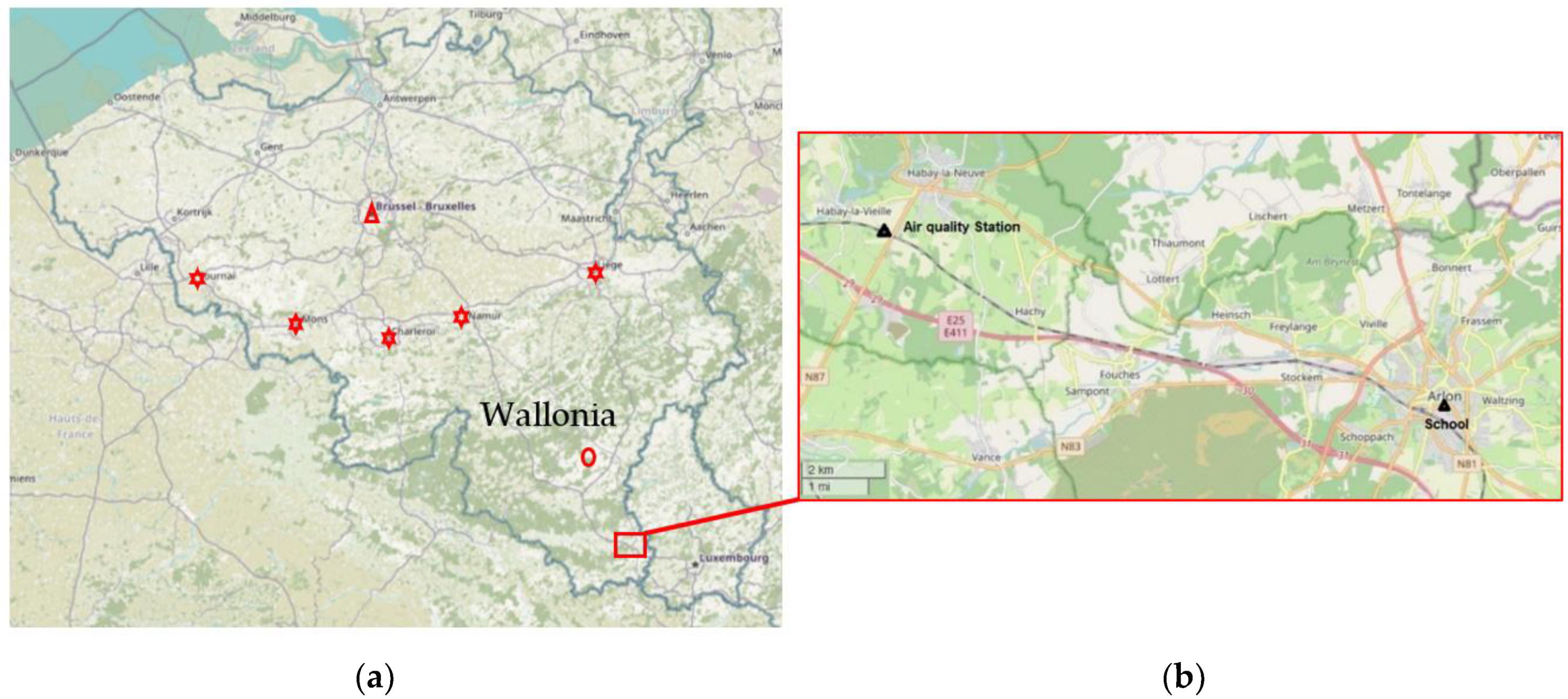
Monitoring of PM2.5 concentrations was conducted around a school in the town of Arlon (49°68′ N; 5°81′ E), 166 km to the south of Brussels (Figure 1).

Figure 1.
(a) Map showing Belgium and the Grand Duchy of Luxembourg. Wallonia is one of three regions in Belgium. Stars indicate the largest cities in Wallonia; the triangle marks the capital, Brussels; and the circle is the meteorological station of Sainte-Ode. (b) Detail map showing Arlon and Habay-la-Vieille with its reference station. Map data © OpenStreetMap contributors, CC BY-SA.
The school has about 1950 primary and secondary students. Arlon lies at an altitude of 426 m a.s.l. The climate is temperate-oceanic, and the annual average temperature is 9 °C with an average in winter of 0.7 °C and 17.7 °C in summer. Average annual rainfall is 839.7 mm [24]. Land use around Arlon city is mostly farmland (yellow) and forest (green) (Figure 2).
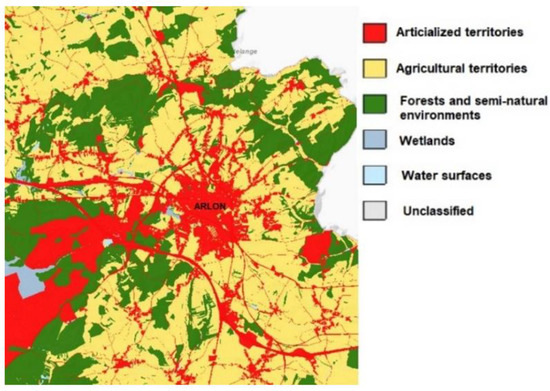
Figure 2.
Land use around Arlon (Service Public de Wallonie, COSW 2007 (1 January 2008). Scale 1/75.000. Produced by Claudia Falzone. Using Cigale © SPW—2021 (13 January 2021)).
Whereas Brussels, also the capital of the EU, has 7392.96 inhabitants/km2 [25], Arlon has 251 [26]. There are no factories or big commercial areas in its center, and the main cause of vehicular traffic is schools, and once a week the market (Thursday) draws people from the surrounding area. Half the people in Arlon work in the Grand Duchy of Luxembourg (52%, distance between Arlon center and nearest border: 3.66 km), 35% work in the city, and 13% work outside the city [27]. Due to its proximity to the Grand Duchy of Luxembourg, Arlon is also a transit city for other border workers.
This school, Institut Notre-Dame d’Arlon, was chosen as a study site for its urban characteristics. It is bounded by three streets and situated in the city center (Figure 3). It was built on a slope, so the streets are at different elevations.
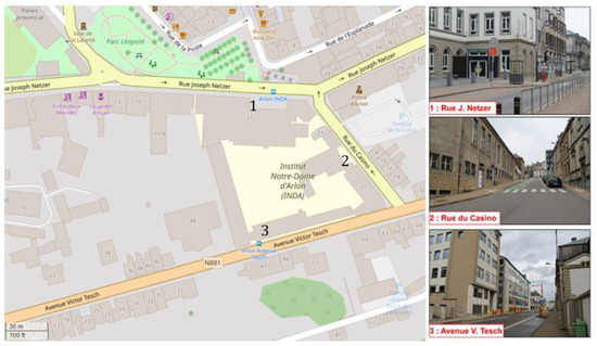
Figure 3.
Sampling site: a primary and secondary school in Arlon bounded by three streets [28]. Numbers indicate the position of the sampling devices. Map data © OpenStreetMap contributors, CC BY-SA.
- Rue Joseph Netzer (hereafter “Netzer”) is a one-way street in front of the main entrance to the secondary school section: altitude 411 m;
- Rue du Casino, (hereafter “Casino”) is a one-way street in front of the main entrance to the primary school section. The street rises 8.7% southeast to northwest;
- Avenue Victor Tesch, (hereafter “Tesch”) is two-way street in front of the second entrance of the secondary school section: altitude 400 m.
2.2. Material
2.2.1. PM2.5 Monitoring––Low-Cost Sensors
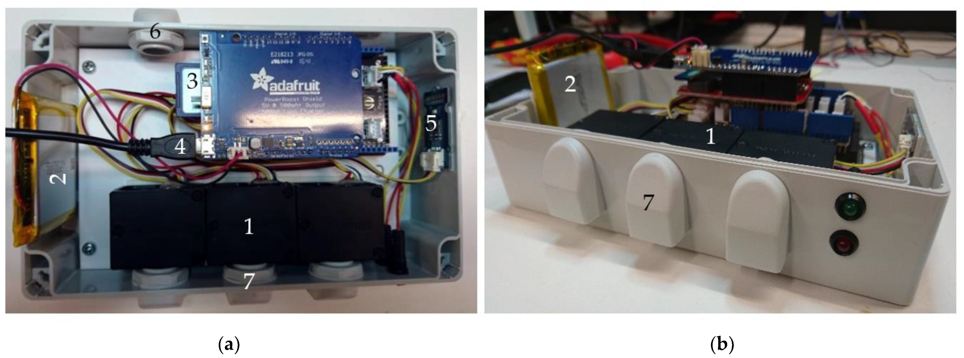
The concentrations of PM2.5 around the school were measured using devices developed by the University of Liege––Sensing of Atmospheres and Monitoring (ULiège–SAM) and called “3PM” (Figure 4). These devices were composed of three battery-run Honeywell PM2.5 optical sensors (HPMA115S0) that had an operating time of about 10 h. Charging time was about 14 h. Data from each sensor were recorded on an SD card with a time step set to one minute.
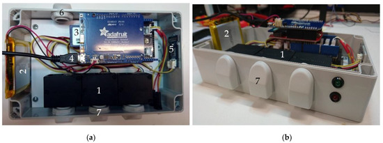
Figure 4.
“3PM” device developed by the University of Liege. (a) Internal view with: 1. Tree Honeywell HPMA115S0 sensors, 2. Battery, 3. SD card, 4. µUSB connector for charging, 5. Temperature (°C)/relative humidity (%) and pressure (hPa), 6. Air outlet and 7. Air inlet. (b) Front of the instrument.
The three devices were placed around the school: one on each street above an entrance. To avoid the influence of the properties of each device, they were rotated among the three sites.
The PM2.5 concentrations from the three sensors were averaged, and all data treatment was carried out on these averaged values. To prevent the influence of extreme values, a data filtering system was set up based on the accuracy values of the sensors provided by the manufacturer (0–100 µg/m3 = ±15 µg/m3; 100–1000 µg/m3 = ±15%) [29]:
- The median of the three sensors was calculated for each time step;
- If a sensor value differed by 15 µg/m3 (median less than 100 µg/m3) or 15% (median greater than 100 µg/m3), the value was rejected as likely being due to sensor fouling. Otherwise, the three values were conserved.
The performance evaluation of the devices was carried out according to the method user guide [30] described in a previous paper [31]. For concentrations below 18 µg/m³, the three devices have an expanded uncertainty of 11%, 15% and 14% for the device 1, 2 and 3 respectively. According to the equivalence method, bellow 25%, no correction is required. For concentrations above 18 µg/m³, a correction is necessary to reach the expended uncertainties of 22%, 26% and 23% for the device 1, 2 and 3 respectively. The majority of the concentrations measured during the containment period were below 18 µg/m³, therefore no correction was necessary.
2.2.2. Traffic Monitoring
The traffic was measured with three TMS-SA units (from iCOMS) (precision or accuracy: speed, ±3 km/h at <100 km/h and 3% at >100 km/h; classification, ±10% (max. four lengths classes); counting, ±3%). The three units were lent by the Scientific Institute of Public Service (ISSeP) and located in each street in compliance with the conditions of placement given by the provider (placed in determining height and at a certain distance of pedestrian crossing and parking areas). The dataset included average speed, the number of light-duty and heavy-duty vehicles, and the total number of vehicles at 1 min intervals.
2.2.3. PM2.5––Reference Monitoring Station
The background concentration of PM2.5 was monitored by a GRIMM EDM180, an instrument certified equivalent to the reference gravimetric method according to the “Guidance for the Demonstration of Equivalence of Ambient Air Monitoring Methods” (European reference) [30]. The official air quality monitoring station nearest to Arlon is the one at Habay-la-Vieille (“Habay”), about 14 km from Arlon (Figure 1b). This rural air quality station is the southernmost in Belgium.
The PM2.5 dataset was extracted for the period 1 January 2017 to 30 September 2020 in a half-hourly format from the wallonair website https://www.wallonair.be/fr/ (accessed on 9 October 2020); data were published by the Walloon Air and Climate Agency (AwAC) and ISSeP.
Meteorological data were collected from the Sainte-Ode station about 34 km from Habay. The weather variables could explain a decrease in PM2.5 concentrations resulting either from dispersion or precipitation.
2.3. Measurement Campaign
The measurement campaign was carried out from 17 March to 25 June 2020. During this period, PM2.5 concentrations and traffic were monitored at the same time.
On the basis of communications from the Belgian National Security Council [32], a timetable for the various reopening periods was drawn up.
- Conf1: (17 March to 14 April 2020) lockdown;
- Conf2: (15 April to 03 May 2020) reopening of the DIY shops and resumption of building work;
- P1A: (4 May to 10 May 2020) reopening of industries;
- P1B: (11 May to 17 May 2020) reopening of shops;
- P2: (18 May to 7 June 2020) reopening of museums and zoos, resumption of outdoor sports (club), authorization to see each other in private, reopening of schools but only for students in the final cycle (primary and secondary);
- P3: (8 June to 14 June 2020) personal bubble increased to 10 people, reopening of hotels, restaurants, and catering (HoReCa) sectors, resumption of indoor sports;
- P4: (from 15 June) reopening of borders.
The three “3PM” devices did not work continuously during the campaign for the following reasons: lifetime of the battery, interdiction on going out due to strict lockdown, and rainy days when devices must be shut off. The summary of the active days is presented in Table 1. Generally, the daily measurements began between 07:00 and 08:00 and ended between 16:00 and 17:00.

Table 1.
Measurement campaign of PM2.5 concentrations around urban school.
Traffic was measured from 25 March to 22 June 2020 (the loan of the instruments stopped on this date). For Casino, the instrument did not work from 22 April at 10:00 to 23 April at 11:00 because of a dead battery.
2.4. Data Treatment
Due to the non-normality of the dataset, a non-parametric Mann–Whitney Wilcoxon test was chosen to compare the values statistically. This test allowed the comparison of datasets two by two on the basis of their medians. The Holm correction was applied to the p-values.
All the data treatment was realized with RStudio (v.1.3.1093)-R (v.4.0.2) [33]. The following packages were used: “lubridate” [34] (inherent in the handling of dates), “reshape2” [35] (contains functions useful for formatting datasets), “ggplot2” [36] (graphics), “ggpubr” [37] (graphics including statistics), “viridis” [38] (color palette), “openair” [39] (time average and wind roses).
3. Results and Discussion
3.1. Background PM2.5 Concentrations—Time Evolution
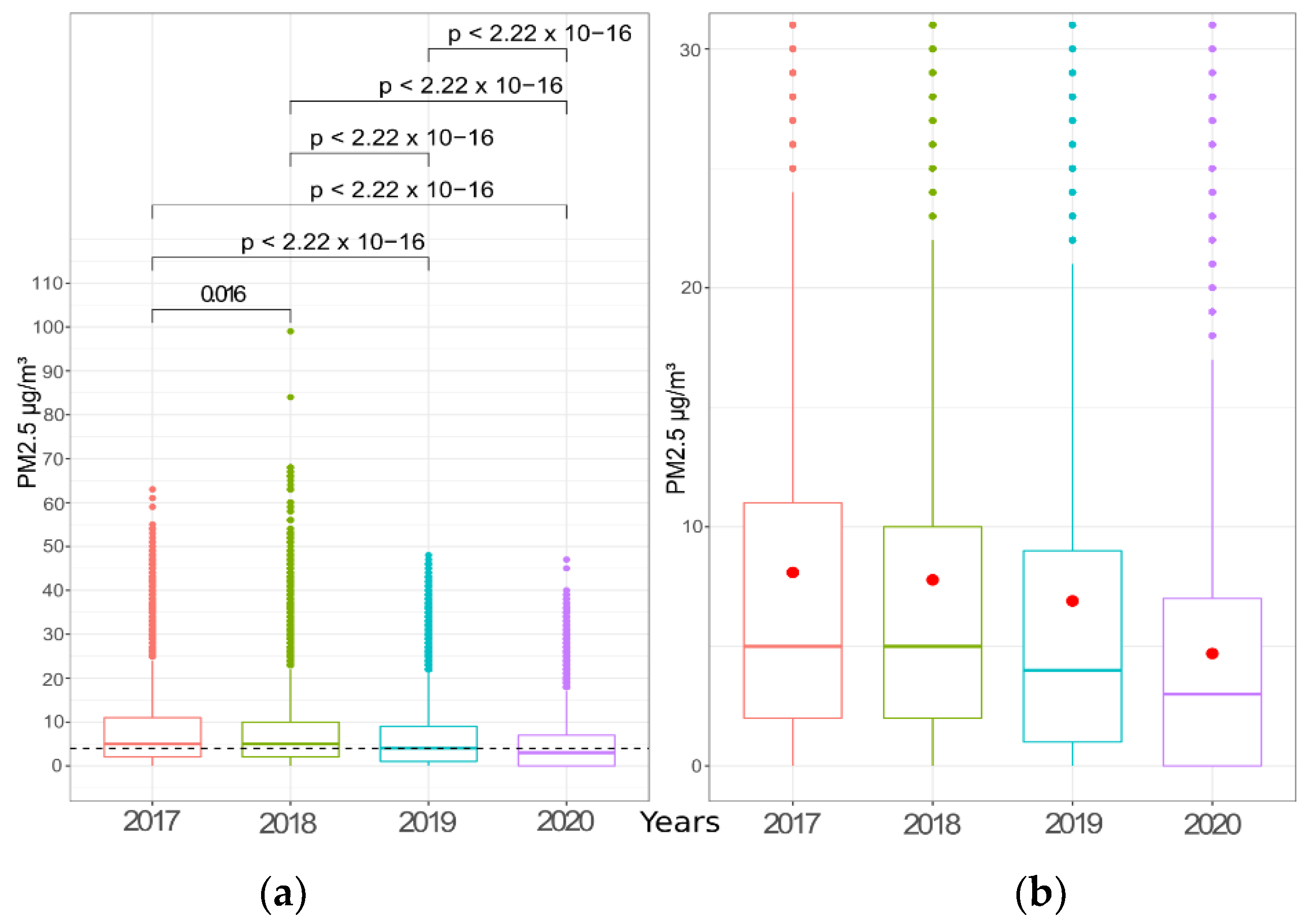
The background PM2.5 concentrations of the Habay station were analyzed from January to September for the years 2017–2020 (the 2020 period was the time of the Arlon measurement campaign). This analysis highlighted a change in PM2.5 concentrations during the last years before the pandemic. Figure 5 shows the boxplots of PM2.5 concentrations for January to September with p-values from the statistical tests and the median for all years (4 µg/m3—dashed line). Significant reductions were observed between each couple of years. The box bounded by the 25–75% interquartile range included lower values in recent years, and the averages decreased over time: 8.1, 7.8, 6.9, and 4.7 µg/m3 for 2017, 2018, 2019, and 2020, respectively.
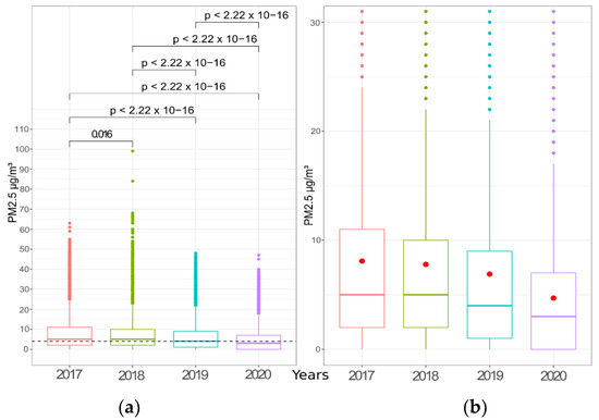
Figure 5.
Comparison among the four years for the period January to September for the Habay air quality station (rural station). The p–values are the results of a Mann–Whitney Wilcoxon pairwise test with the Holm correction (αthreshold = 0.05). The dashed line corresponds to the median (4 µg/m3) of the four years for the period. (a) complete dataset; (b) detail from 0 to 30 µg/m3; averages in red points.
The explanatory variables for the decrease in PM are numerous: rain (washing effect), favorable atmospheric stability, wind direction, or anthropogenic activity. For this Habay dataset, only rain was known, so a potential PM diminution trend corresponding to rainy days was investigated. Days without rain (0 mm) were added up for each 273-day period (January to September) for each year: 2017: 131/273 (48%, 1 NA); 2018: 156/273 (58%, 2 NAs); 2019: 138/273 (51%, 2 NAs) and 2020: 151/274 (55%, 0 NA). In fact, the number of rain-free days per year did not seem to explain the decrease in PM2.5 concentrations over time. Further investigation should be added to understand the complexity of the PM pollution evolution over several years, but that is not the objective of this work.
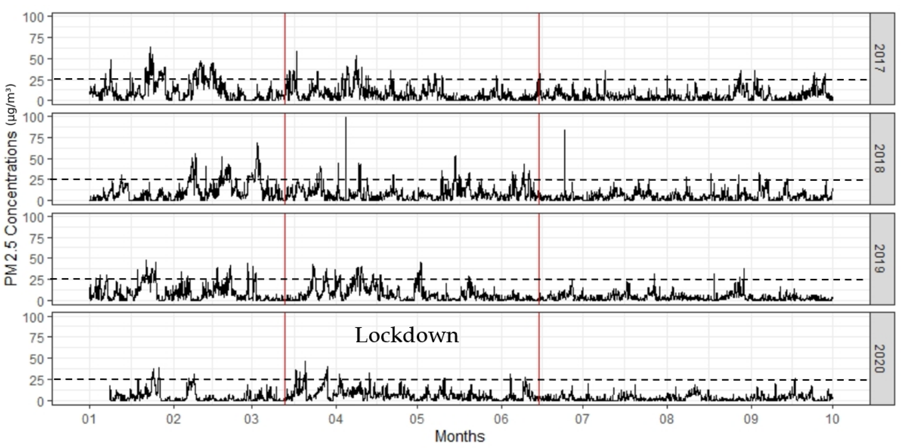
In 2020, the period before the lockdown (Figure 6, left red line) shows that the concentrations were lower than in the other years. During the lockdown, some episodes of concentration higher than 25 µg/m3 (dashed line) were unexpectedly observed. After 15 June, when containment ended (Figure 6, right red line), the frequency of concentrations below 12 µg/m3 was surprisingly lower than during the containment and lower for 2020 than for the other years.
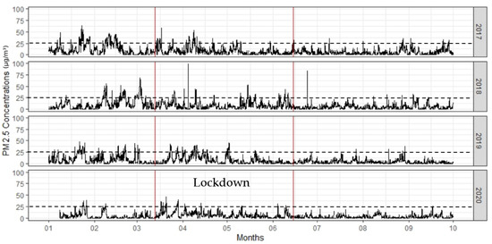
Figure 6.
PM2.5 concentrations from 1 January to 30 September in different years. The red lines delimitate the lockdown period for 2020, from 13 March to 15 June. The dashed line: PM2.5 limit value in 2020.
3.2. Weather Conditions—Before, during, and after the Lockdown
Among the four years analyzed, 2020 had the lowest PM2.5 concentrations. These results are in agreement with the study carried out by the ISSeP at the quality monitoring station in Charleroi (Figure 1, urban station) [20]. The authors of the report also presented conditions from the Sainte-Ode station, which is not very far from Habay, so its data may be considered as representative of the weather conditions at Habay for the periods before, during, and after lockdown:
- Before lockdown: winds were predominantly from the southwest with a higher average wind speed than in previous years. Precipitation was heavier and more frequent. These meteorological conditions were largely favorable to good air quality, which explains the differences in PM2.5 concentrations compared with previous years [20].
- During lockdown: the weather was dry, sunny with continental currents (ENE), which were not favorable to good air quality, especially in the spring when particulate matter peaks are more frequent, particularly due to agricultural activity [20]. However, the PM2.5 concentrations at the Habay station were lower than for previous years. One explanation could be the reduction of human activity like driving. Another explanation could be that the wind direction did not transport ambient air from the highway (source of PM2.5) to the measurement station (Figure 2, highway E25/E411). Despite this observation, there were some peaks of concentration. Indeed, an ENE wind could have transported PM from agricultural areas, the village of Habay-la-Neuve, or forests (pollen emission).
- After lockdown: Weather conditions were identical to what they were during confinement, i.e., unfavorable for good air quality with a risk of particulate peaks typical of spring [20]. The unexpected low PM2.5 concentrations, observed in Figure 6, were probably due to the decrease in agricultural activity (spreading activity), wind direction, and teleworking still being in force.
3.3. Evolution of Traffic between 2019 and 2020 during the Confinement in Arlon
The first traffic measurement campaign in Arlon was held from 17 April to 2 May 2019 inclusive. The second, from 25 March to 21 June 2020, started later than the PM2.5 concentration campaign (17 March to 25 June).
The comparison of traffic between 2019 and 2020 was carried out for the period from 17 April to 2 May. The 2019 period covered seven days of school holidays and nine school days, and 2020 covered 16 days during Conf2 and one public holiday. As shown in Figure 7, the number of vehicles was significantly different for the same period. A decrease was observed from 2019 to 2020 (about 60% for the three streets). These observations were in agreement with the observations made in other countries during the lockdown [16]. This reduction clearly showed the impact of containment on traffic.
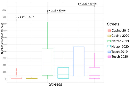
Figure 7.
Comparison between measurement traffic campaigns taken in 2019 and 2020 (17 April–2 May, inclusive); p–values were the results of Mann–Whitney Wilcoxon pairwise tests with the Holm correction (αthreshold = 0.05).
To better understand the PM2.5 results in Arlon (cf. Section 3.3), it is necessary to consider the distribution of traffic among the three streets. Under normal conditions, Casino had a frequency rate about 80% lower than that of Netzer and Tesch, which presented the same frequency profiles. Even after the reopening of DIY shops and construction trades, the number of vehicles did not return to 2019 levels despite the holiday period.
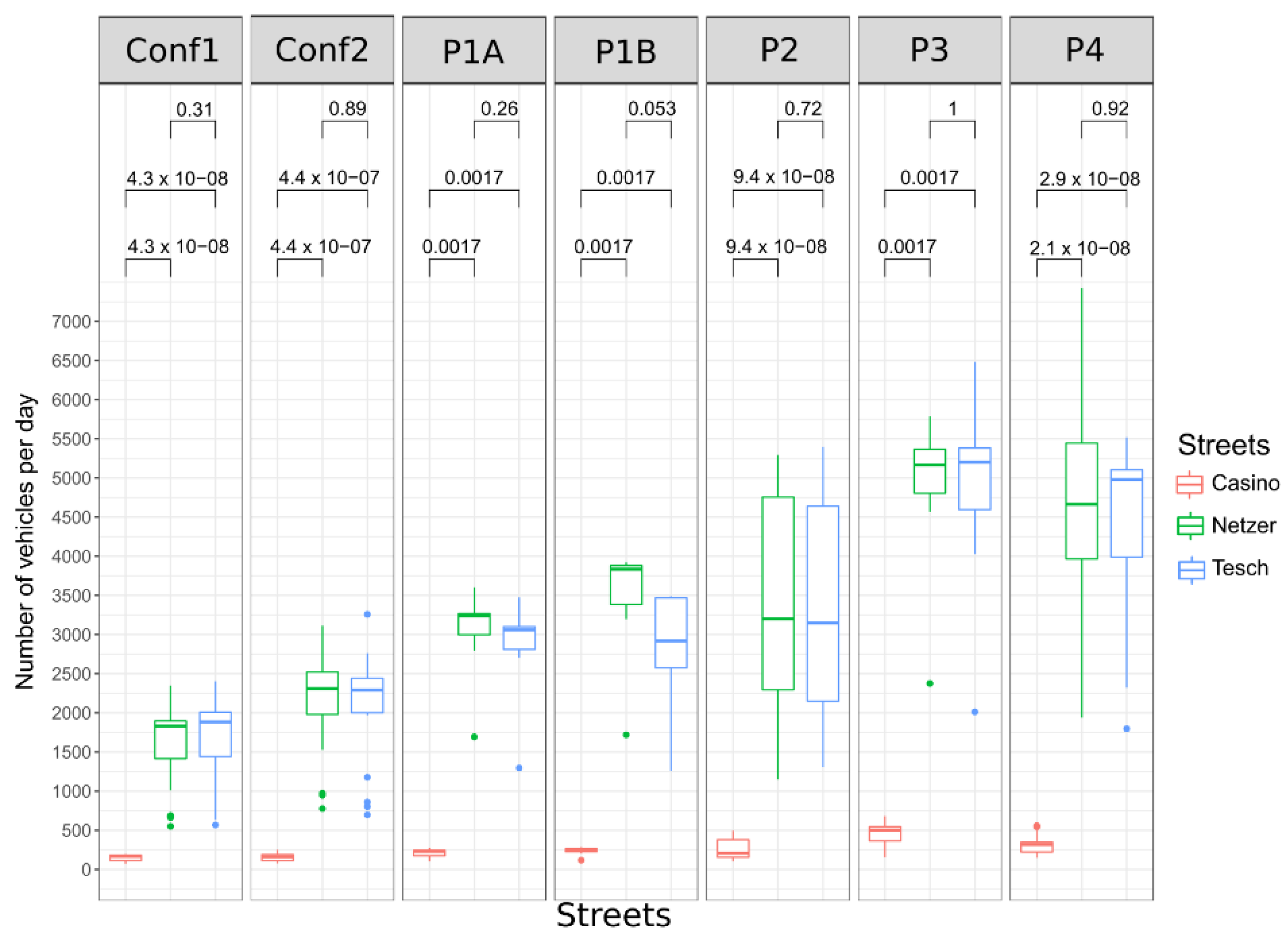
In general, traffic on each street increased during the different reopening periods (Figure 8). During weekends, the number of vehicles decreased in Arlon for each period (Figure S1). The same observation was made for Wednesday, mainly because for Belgian schools it is a half-day, and those who work part-time take the day off (Figure S1).
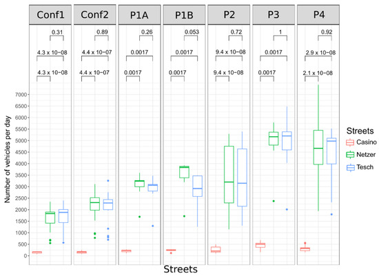
Figure 8.
The sum of vehicles per day for each period. The p–values are the results of a Mann–Whitney Wilcoxon pairwise test with the Holm correction (αthreshold = 0.05).
3.4. PM2.5 Concentration in Arlon–Evolution and Explanations
During the lockdown, the PM2.5 concentrations measured at Arlon should have been similar to the background concentrations measured at the reference Habay station if the winds were from the NW or the reverse (NW–SE axis Habay–Arlon, Figure 1), or if the ambient air were not affected by local pollution. Variations between the two sites could be explained by a difference in wind direction, but also by specific local events. For each period, an analysis was performed to identify the possible causes of the concentration variations. The evolution of the PM in the Arlon streets was presented as well as the relationship among the three streets.
Each period was determined by the number of days, not by the number of observations (i.e., P1A is represented by days 4, 5, and 8 for Netzer; days 5 and 6 for Casino; days 4, 6, and 8 for Tesch; days 4, 5, 6, and 8 for Habay). For the same period, the measured days could be different due to a device being out of order (Table 1); however, the number of days was the same for each site (except for P1A and P1B). The number of measurements depended on the battery life of the devices.
PM2.5 on the three streets of Arlon and in Habay (Table S1) decreased over the periods, but this was not related to traffic, which increased according to the stoppage and opening of human activities. The PM2.5 reduction was probably due to factors that could not be formally identified in this study.
Moreover, a positive correlation was observed for PM2.5 concentration means in each period between each street and the Habay station. However, there were differences that could be explained by wind direction (opposite from Habay), local events in the streets (building work), and agricultural activity (Figure S2).
For each period, a detailed explanation was proposed to understand if the lockdown were responsible for a decrease or increase in PM2.5 concentrations.
During the Conf1 period (17 March–14 April), before the reopening (Figure S3), PM2.5 concentrations in Habay and on the streets of Arlon were similar despite the dominant winds coming mainly from E/ENE.
In contrast, the Conf2 period (15 April–5 May), the reopening of DIY shops and resumption of building work (Figure S4), showed a 1 µg/m3 increase relative to the background levels for the couples Habay–Casino and Habay–Netzer, while the dominant winds were the same as during Conf1. The explanation is probably linked to the resumption of construction at the intersection of the two streets. Moreover, the construction work was located to the east of the devices in the direction of the wind. The construction site could have been a source of PM2.5 from dust and lorry traffic. At the announcement of the containment, construction was interrupted during the last phase of structural works.
For the P1A period (4–10 May), the reopening of industries (Figure S5) showed a 5 µg/m3 increase for Netzer in the couples Casino–Netzer and Habay–Netzer and a 3 µg/m3 increase for Netzer–Tesch even though the prevailing winds were from a similar direction as for Conf1 and Conf2. The higher concentration in Netzer could be explained by the poor dispersal of pollutants because low wind speed was observed during construction activity.
During the P1B period (11–17 May), the reopening of shops (Figure S6) showed a 3 µg/m3 increase relative to background levels for the couple Netzer–Habay and 2 µg/m3 for Tesch–Habay. Higher traffic on Tesch and Netzer, coupled with low wind speeds from the NNE/ENE, might have been responsible for the higher PM2.5 concentrations in the two streets.
In the P2 period (18 May–7 June), the reopening of museums and zoos, resumption of outdoor sports (club), authorization to see each other in private, reopening of schools for primary and secondary students in their final cycle (Figure S7) showed 1 µg/m3 increase relative to background levels for the couple Casino–Habay, and 2 µg/m3 for the couples Netzer–Habay and Tesch–Habay. There was no dominant wind direction, and wind speeds were mostly slow. Street traffic could explain these slight differences in concentration.
During the P3 period (8–14 June), when the personal bubble increased to 10 people, the HoReCa sector reopened, and indoor sports resumed (Figure S8), measurements of PM2.5 concentrations in Habay for the first time showed an increase compared to previous periods (Table S1). Moreover, no significant differences were observed between Arlon and Habay, which went against our expectations. Indeed, following the relaxing of health constraints (especially those related to schools: number of students that is allowed, extended class hours, resumption of face-to-face teaching), we expected to see a more marked increase for Arlon. Similarities in concentrations could be explained by the wind direction, WNW/ESE, the Habay–Arlon axis.
The P4 period (from 15 June), when borders reopened (Figure S9) showed different increases for the following couples: 1 µg/m3 for Netzer (Casino–Netzer and Netzer-Tesch), 3 µg/m3 for Casino (Casino–Habay), 4 µg/m3 for Netzer (Netzer-Habay), and 3 µg/m3 for Tesch (Tesch-Habay). The concentrations measured in Habay were low despite the southwest wind’s bringing ambient air from the highway. Therefore, traffic from the highway did not seem to impact the concentrations measured in Habay. Actually, at that time, working from home was still in force in Belgium and in the Grand Duchy of Luxembourg, and the traffic on this highway, which is mainly used by cross-border Luxembourger workers, was probably lower than usual. The higher PM2.5 concentrations in Netzer could have been the result of a traffic peak (Figure S1) due to school exams. The wind direction and the positive slope of Casino street could explain the low pollution dispersion.
As the reopening progressed, the mean number of vehicles per 30 min increased for each street (Figure S10). The traffic on Netzer and Tesch streets increased more or less equally over time (Spearman coefficient ρ = 0.66, Figure S11). However, this observation did not apply to Casino–Netzer or Casino–Tesch: ρ = 0.29 and ρ = 0.30, respectively (Figure S11). Background PM2.5 levels did not appear to behave similarly to traffic density over time (Figure S10). The background concentration was removed from the PM2.5 concentrations measured for each street and compared to the traffic (Figure S11). The concentrations fit very well between them but no correlation could be found between PM2.5 concentrations (street concentration minus background concentration) and the level of traffic (sum of vehicles per 30 min): ρ = 0.028, 0.029 and 0.026 for Casino, Netzer, and Tesch, respectively (Figure S11). This lack of correlation was probably due to: (i) the fact that the number of vehicles on the roads of southern Belgium did not return to the number for previous years (see 3.2), and (ii) the low contribution of traffic to the formation of PM2.5 (17% for Wallonia [20]). In Arlon, climatic conditions and fertilizer application in spring during dry weather seemed to be the most influential factors for PM2.5 concentrations.
4. Conclusions
At the rural station in Habay-la-Vieille, the last few years have been marked by a downward trend in measurements of background PM2.5 concentrations. The year 2020, a special year due to the confinement, showed even lower concentrations from January to September than for previous years. However, it was not obvious that the confinement (traffic reduction, decrease in human activity) was the main explanation. Indeed, the report “Impact du confinement Covid-19 sur la qualité de l’air en Région wallone” [20] explained that the confinement and the reduction of road traffic did not reduce PM2.5 concentrations in Wallonia by very much. In contrast, the weather played a considerable role. The beginning of the year (before the lockdown) brought conditions favorable to good air quality, which explained the low concentrations of PM2.5 compared to previous years. Unexpectedly, the lockdown period showed higher average concentrations than the pre-lockdown period. The meteorological conditions were unfavorable to good air quality, probably because of agricultural activities.
This study aimed to understand the situation near a school in a small rural town (Arlon). A PM2.5 measurement campaign was tied to a traffic count from 17 March to 22 June 2020. It turned out that over the entire period there was no correlation between traffic and PM2.5 concentrations. However, detailed analysis of each period revealed that it was possible to observe slight significant differences between the background concentrations measured in Habay and in Arlon (variation between 1 and 5 µg/m3 for the streets). For some of these differences, traffic nevertheless could have played a local role because the differences in the maximum values between Habay and Netzer were 30 µg/m3 for the P2 period. The construction site located near the entrance of the school and the weather conditions (low wind speed) also explained these differences. It is important to note that the level of traffic, even at the end of the reopening, did not return to the 2019 level. Indeed, schooling resumed in a restrictive manner (no 100% attendance for any classes) and working from home was still in place for office work.
To determine the correct contribution of traffic to the PM2.5 emissions around the school, this experiment could be replicated by considering both school and non-school periods. It could be accompanied by a study of the composition of the particles according to the different periods of the year (not only the spring but also the winter, during which time domestic heating is an important PM2.5 source).
Following this study, it seemed that the containment did not improve PM2.5 concentrations in a small rural city. Indeed, after the containment, concentrations remained relatively low despite the increase in human activity. This was in line with the findings for Wallonia and can be explained by exceptional weather conditions.
Supplementary Materials
The following are available online at https://www.mdpi.com/article/10.3390/atmos12101333/s1, Table S1: Statistics of PM2.5 concentrations (µg/m3) for each period; Figure S1: Traffic evolution over time for the three streets: Casino, Netzer, and Tesch. The number of vehicles corresponds to the sum per day for each street; Figure S2: Comparison among PM2.5 concentrations (µg/m3) of each site and by period; Figure S3: Comparison among the three streets and Habay for Conf1. n = number of observations and order = x-axis labels. The p-values are the results of a pairwise Mann–Whitney Wilcoxon test with Holm correction. The wind rose shows the wind directions and speeds for Conf1 from 06:00 to 18:00 (data from the Sainte-Ode at 30 m height); Figure S4: Comparison among the three streets and Habay for Conf2. n = number of observations and order = x-axis labels. The p-values are the results of a pairwise Mann–Whitney Wilcoxon test with Holm correction. The wind rose shows the wind directions and speeds for Conf2 from 06:00 to 18:00 (data from the Sainte-Ode at 30 m height); Figure S5: Comparison among the three streets and Habay for P1A. n = number of observations and order = x-axis labels. The p-values are the results of a pairwise Mann–Whitney Wilcoxon test with Holm correction. The wind rose shows the wind directions and speeds for P1A from 06:00 to 18:00 (data from the Sainte-Ode at 30 m height); Figure S6: Comparison among the three streets and Habay for P1B. n = number of observations and order = x-axis labels. The p-values are the results of a pairwise Mann–Whitney Wilcoxon test with Holm correction. The wind rose shows the wind directions and speeds for P1B from 6:00 to 18:00 (data from the Sainte-Ode at 30 m height); Figure S7: Comparison among the three streets and Habay for P2. n = number of observations and order = x-axis labels. The p-values are the results of a pairwise Mann–Whitney Wilcoxon test with Holm correction. The wind rose shows the wind directions and speeds for P2 from 06:00 to 18:00 (data from the Sainte-Ode at 30 m height); Figure S8: Comparison among the three streets and Habay for P3. n = number of observations and order = x-axis labels. The p-values are the results of a pairwise Mann–Whitney Wilcoxon test with Holm correction. The wind rose shows the wind directions and speeds for P3 from 06:00 to 18:00 (data from the Sainte-Ode at 30 m height); Figure S9: Comparison among the three streets and Habay for P4. n = number of observations and order = x-axis labels. The p-values are the results of a pairwise Mann–Whitney Wilcoxon test with Holm correction. The wind rose shows the wind directions and speeds for P4 from 06:00 to 18:00 (data from the Sainte-Ode at 30 m height); Figure S10: Time plots of the mean of vehicles per 30 min, the concentration of PM2.5 measured at Habay-la-Vieille, and the rain quantity measure in mm. Each period is represented by a vertical dashed line; Figure S11: Correlation between PM2.5 concentrations in µg/m3 and the traffic level for each site (sum of vehicles/30 min). The Spearman coefficient is shown in the upper panel.
Author Contributions
Conceptualization, C.F.; methodology, C.F. and J.M.; code development, C.F. and J.M.; validation, C.F., A.-C.R. and J.M.; formal analysis, C.F.; investigation, J.M.; resources, A.-C.R.; data curation, C.F.; writing—original draft preparation, C.F.; writing—review and editing, C.F.; supervision, A.-C.R. All authors have read and agreed to the published version of the manuscript.
Funding
This research received no external funding.
Institutional Review Board Statement
Not applicable.
Informed Consent Statement
Not applicable.
Data Availability Statement
The PM2.5 dataset from the ISSeP stations was extracted from the wallonair website https://www.wallonair.be/fr/ (accessed on 9 October 2020); The PM2.5 dataset from our instruments are not published.
Acknowledgments
The authors would like to thank M. Dury, F. Lenartz and N. Fernemont from ISSeP, the city of Arlon, the school (INDA) and L. Collard.
Conflicts of Interest
The authors declare no conflict of interest.
References
- European Environment Agency. Air Quality in Europe: 2020 Report; European Environment Agency: København, Denmark, 2020. [Google Scholar]
- Goodsite, M.E.; Hertel, O.; Johnson, M.S.; Jørgensen, N.R. Urban Air Quality: Sources and Concentrations. In Air Pollution Sources, Statistics and Health Effects; Goodsite, M.E., Johnson, M.S., Hertel, O., Eds.; Springer: New York, NY, USA, 2021; pp. 193–214. ISBN 9781071605950. [Google Scholar]
- U.S. Environmental Protection Agency. Health and Environmental Effects of Particulate Matter (PM). Available online: https://www.epa.gov/pm-pollution/health-and-environmental-effects-particulate-matter-pm (accessed on 9 February 2021).
- Daellenbach, K.R.; Uzu, G.; Jiang, J.; Cassagnes, L.-E.; Leni, Z.; Vlachou, A.; Stefenelli, G.; Canonaco, F.; Weber, S.; Segers, A.; et al. Sources of particulate-matter air pollution and its oxidative potential in Europe. Nat. Cell Biol. 2020, 587, 414–419. [Google Scholar] [CrossRef]
- Steenhof, M.; Gosens, I.; Strak, M.; Godri, K.J.; Hoek, G.; Cassee, F.R.; Mudway, I.S.; Kelly, F.J.; Harrison, R.M.; Lebret, E.; et al. In vitro toxicity of particulate matter (PM) collected at different sites in the Netherlands is associated with PM composition, size fraction and oxidative potential–The RAPTES project. Part. Fibre Toxicol. 2011, 8, 26. [Google Scholar] [CrossRef] [PubMed] [Green Version]
- Air Quality Guidelines: Global Update 2005: Particulate Matter, Ozone, Nitrogen Dioxide, and Sulfur Dioxide; World Health Organization (Ed.) World Health Organization: Copenhagen, Denmark, 2006; ISBN 9789289021920. [Google Scholar]
- European Parliament and Council Directive 2008/50/CE—Ambient Air Quality and Cleaner Air for Europe. 2008. Available online: https://eur-lex.europa.eu/eli/dir/2008/50/oj/fra?locale=en) (accessed on 18 September 2015).
- European Environment Agency. Air Quality in Europe: 2019 Report; European Environment Agency: København, Denmark, 2019. [Google Scholar]
- Amato, F.; Schaap, M.; Reche, C.; Querol, X. Road Traffic: A major source of particulate matter in Europe. In Urban Air Quality in Europe; Viana, M., Ed.; Springer: Berlin/Heidelberg, Germany, 2013; Volume 26, pp. 165–193. ISBN 9783642384509. [Google Scholar]
- Herich, H.; Hueglin, C. Residential Wood Burning: A Major Source of Fine Particulate Matter in Alpine Valleys in Central Europe. In Urban Air Quality in Europe; Viana, M., Ed.; Springer: Berlin/Heidelberg, Germany, 2013; Volume 26, pp. 123–140. ISBN 9783642384509. [Google Scholar]
- Zalakeviciute, R.; López-Villada, J.; Rybarczyk, Y. Contrasted Effects of Relative Humidity and Precipitation on Urban PM2.5 Pollution in High Elevation Urban Areas. Sustainability 2018, 10, 2064. [Google Scholar] [CrossRef] [Green Version]
- The Convention and Its Achievements|UNECE. Available online: https://unece.org/convention-and-its-achievements (accessed on 17 August 2021).
- Takano, Y.; Moonen, P. On the Influence of Roof Shape on Flow and Dispersion in an Urban Street Canyon. J. Wind Eng. Ind. Aerodyn. 2013, 123, 107–120. [Google Scholar] [CrossRef]
- Vardoulakis, S.; Fisher, B.E.A.; Pericleous, K.; Gonzalez-Flesca, N. Modelling Air Quality in Street Canyons: A Review. Atmos. Environ. 2003, 37, 155–182. [Google Scholar] [CrossRef] [Green Version]
- Zhang, H.; Xu, T.; Wang, Y.; Zong, Y.; Li, S.; Tang, H. Study on the Influence of Meteorological Conditions and the Street Side Buildings on the Pollutant Dispersion in the Street Canyon. Build. Simul. 2016, 9, 717–727. [Google Scholar] [CrossRef]
- Fu, F.; Purvis-Roberts, K.L.; Williams, B. Impact of the COVID-19 Pandemic Lockdown on Air Pollution in 20 Major Cities around the World. Atmosphere 2020, 11, 1189. [Google Scholar] [CrossRef]
- Belgique-PIB-Produit Intérieur Brut 2021. Available online: https://fr.countryeconomy.com/gouvernement/pib/belgique (accessed on 17 August 2021).
- Binamé, A. Coronavirus En Belgique: Augmentation Du Trafic En Ce Début de Semaine. RTBF 2020. Available online: https://www.rtbf.be/services/mobilinfo/detail_coronavirus-en-belgique-augmentation-du-trafic-en-ce-debut-de-semaine?id=10485676 (accessed on 10 February 2021).
- Bruxelles Environnement Evaluation de l’impact Des Mesures Prises Dans Le Cadre de La Pandémie de Covid-19 Sur La Qualité de l’air En Région de Bruxelles-Capitale. 2020, pp. 1–8. Available online: http://environnement.brussels/sites/default/files/user_fihttpsles/rapport_qualite_air_covid-19_06mai2020.pdf (accessed on 2 March 2021).
- ISSeP Impact du Confinement Covid-19 sur la Qualité de L’air en Région Wallonne. 2020, p. 70. Available online: https://www.wallonair.be/images/pdf/rapport_COVID19_final.pdf (accessed on 2 March 2021).
- Utilisation Du Sol | Statbel. Available online: https://statbel.fgov.be/fr/themes/environnement/sol/utilisation-du-sol (accessed on 15 August 2021).
- Bloss, W. Urban Atmospheric Composition Processes. In Air Pollution Sources, Statistics and Health Effects; Goodsite, M.E., Johnson, M.S., Hertel, O., Eds.; Springer: New York, NY, USA, 2021; pp. 215–228. ISBN 9781071605950. [Google Scholar]
- Viatte, C.; Wang, T.; Van Damme, M.; Dammers, E.; Meleux, F.; Clarisse, L.; Shephard, M.W.; Whitburn, S.; Coheur, P.F.; Cady-Pereira, K.E.; et al. Atmospheric Ammonia Variability and Link with Particulate Matter Formation: A Case Study over the Paris Area. Atmos. Chem. Phys. 2020, 20, 577–596. [Google Scholar] [CrossRef] [Green Version]
- Météo et Climat: Arlon (Belgique). Available online: https://planificateur.a-contresens.net/europe/belgique/wallonie/arlon/2803073.html (accessed on 13 August 2021).
- Région de Bruxelles-Capitale. Wikipédia. 2021. Available online: https://fr.wikipedia.org/w/index.php?title=R%C3%A9gion_de_Bruxelles-Capitale&oldid=184940762 (accessed on 15 August 2021).
- Arlon. Wikipédia. 2021. Available online: https://fr.wikipedia.org/w/index.php?title=Arlon&oldid=184976596 (accessed on 15 August 2021).
- Master Students; Devillet, G. Etude d’incidence sur l’environnement Projet “Green District” à Arlon; Department of Geography, University of Liege: Liège, Belgium, 2018; p. 174. [Google Scholar]
- Simon, F. TFE–Les particules PM 2.5: Influence du trafic de dépose scolaire sur la qualité de l’air d’une école. In Modélisation ENVI-Met et Mesures à L’aide de Capteurs «Low Cost»; Arlon Campus: Liège, Belgium, 2019. [Google Scholar]
- Honeywell–International Inc. Honeywell HPM Series–Particulate Matter Sensors; Honeywell–International Inc.: Charlotte, NC, USA, 2021. [Google Scholar]
- Ballesta, P.P.; Febo, A.; Fernandez-Patier, R.; Fröhlich, M.; dos Garcia, S.S.; Hafkenscheid, T.; Jacobi, S.; Meulen, T.; Munns, D.; Pfeffer, H.-U.; et al. Guide to the Demonstration of Equivalence of Ambient Air Monitoring Methods. Available online: https://ec.europa.eu/environment/air/quality/legislation/pdf/equivalence.pdf (accessed on 9 March 2021).
- Falzone, C.; Romain, A.-C.; Broun, V.; Gérard, G. PM2.5 Low-Cost Sensor Performance in Ambient Conditions; Elsevier: Amsterdam, The Netherlands, 2020; ISBN 9783844076288. [Google Scholar]
- National Safety Council–Belgium. Available online: https://www.belgium.be/fr/actualites/overview?f%5B0%5D=publication_year%3A2020&f%5B1%5D=theme%3A65 (accessed on 10 February 2021).
- R Core Team. R: A Language and Environment for Statistical Computing; R Foundation for Statistical Computing: Vienna, Austria, 2020. [Google Scholar]
- Grolemund, G.; Wickham, H. Dates and Times Made Easy with Lubridate. J. Stat. Soft. 2011, 40, 1–25. [Google Scholar] [CrossRef]
- Wickham, H. Reshaping Data with the Reshape Package. J. Stat. Soft. 2007, 21, 1–20. [Google Scholar] [CrossRef]
- Wickham, H. Ggplot2: Elegant Graphics for Data Analysis, 2nd ed.; Springer: Cham, Switzerland, 2016; ISBN 9783319242774. [Google Scholar]
- Kassambara, A. Ggpubr: Ggplot2 Based Publication Ready Plots. 2020. Available online: https://cran.r-project.org/web/packages/ggpubr/index.html (accessed on 6 May 2021).
- Garnier, S. Viridis: Default Color Maps from “Matplotlib”. 2018. Available online: https://scholar.google.com.hk/citations?view_op=view_citation&hl=zh-TW&user=4MNHWX8AAAAJ&sortby=pubdate&citation_for_view=4MNHWX8AAAAJ:Ej9njvOgR2oC (accessed on 6 May 2021).
- Carslaw, D.C.; Ropkins, K. Openair–An R Package for Air Quality Data Analysis. Environ. Model. Softw. 2012, 27–28, 52–61. [Google Scholar] [CrossRef]


Publisher’s Note: MDPI stays neutral with regard to jurisdictional claims in published maps and institutional affiliations. |
© 2021 by the authors. Licensee MDPI, Basel, Switzerland. This article is an open access article distributed under the terms and conditions of the Creative Commons Attribution (CC BY) license (https://creativecommons.org/licenses/by/4.0/).