Abstract
In this study, the applicability of three gridded datasets was evaluated (Climatic Research Unit (CRU) Time Series (TS) 3.1, “Asian Precipitation—Highly Resolved Observational Data Integration Toward the Evaluation of Water Resources” (APHRODITE)_V1101, and the climate forecast system reanalysis dataset (CFSR)) in different combinations against observational data for predicting the hydrology of the Upper Vakhsh River Basin (UVRB) in Central Asia. Water balance components were computed, the results calibrated with the SUFI-2 approach using the calibration of soil and water assessment tool models (SWAT–CUP) program, and the performance of the model was evaluated. Streamflow simulation using the SWAT model in the UVRB was more sensitive to five parameters (ALPHA_BF, SOL_BD, CN2, CH_K2, and RCHRG_DP). The simulation for calibration, validation, and overall scales showed an acceptable correlation between the observed and simulated monthly streamflow for all combination datasets. The coefficient of determination (R2) and Nash–Sutcliffe efficiency (NSE) showed “excellent” and “good” values for all datasets. Based on the R2 and NSE from the “excellent” down to “good” datasets, the values were 0.91 and 0.92 using the observational datasets, CRU TS3.1 (0.90 and 0.90), APHRODITE_V1101+CRU TS3.1 (0.74 and 0.76), APHRODITE_V1101+CFSR (0.72 and 0.78), and CFSR (0.67 and 0.74) for the overall scale (1982–2006). The mean annual evapotranspiration values from the UVRB were about 9.93% (APHRODITE_V1101+CFSR), 25.52% (APHRODITE_V1101+CRU TS3.1), 2.9% (CFSR), 21.08% (CRU TS3.1), and 27.28% (observational datasets) of annual precipitation (186.3 mm, 315.7 mm, 72.1 mm, 256.4 mm, and 299.7 mm, out of 1875.9 mm, 1236.9 mm, 2479 mm, 1215.9 mm, and 1098.5 mm). The contributions of the snowmelt to annual runoff were about 81.06% (APHRODITE_V1101+CFSR), 63.12% (APHRODITE_V1101+CRU TS3.1), 82.79% (CFSR), 81.66% (CRU TS3.1), and 67.67% (observational datasets), and the contributions of rain to the annual flow were about 18.94%, 36.88%, 17.21%, 18.34%, and 32.33%, respectively, for the overall scale. We found that gridded climate datasets can be used as an alternative source for hydrological modeling in the Upper Vakhsh River Basin in Central Asia, especially in scarce-observation regions. Water balance components, simulated by the SWAT model, provided a baseline understanding of the hydrological processes through which water management issues can be dealt with in the basin.
1. Introduction
Watershed-based hydrological models provide a practical approach to evaluating the water cycle’s components, particularly snowmelt’s contribution to river flow [1,2]. One of the challenges in mountainous regions when modeling watershed hydrology and evaluating water balance components is obtaining weather input data, which are generally among the most essential drivers of watershed models [3]. Unfortunately, observational climate stations are often sparsely located and thus cannot characterize the climate conditions throughout a catchment, particularly if large hydroclimatic gradients exist. Additionally, climate station measurements often do not cover the proposed modeling period, and there may be gaps in the records. In order to solve this issue, the investigation of alternative climate data is essential in mountainous areas.
The applicability of the climate forecast system reanalysis (CFSR), “Asian Precipitation—Highly Resolved Observational Data Integration Toward the Evaluation of Water Resources” (APHRODITE), and Climatic Research Unit (CRU) datasets for hydrological models in water balance components analysis has not been investigated thus far in the UVRB. Similarly, previous studies on the applicability of models to estimate hydrological components in the highlands of Tajikistan (UVRB) in Central Asia have not been conducted. Various hydrological models at the watershed scale have been used for the estimation of water cycle components, including the Hydrologic Engineering Center hydrologic modeling system [4], MIKE SHE [5], the soil and water assessment tool [6], the hydrologic simulation program Fortran [7], and the snowmelt runoff model [2]. The SWAT model is internationally recognized as a robust hydrological model and is widely used, including in several basins that have snowmelt-dominated streamflow [8,9,10,11,12,13,14].
Previous research indicated that the SWAT model is a common tool to assess the water balance components of watersheds. Combinations of CFSR datasets with the SWAT model and observational datasets with the SWAT model were applied to different watersheds in the Blue Nile Basin in Ethiopia to assess water-balance components, particularly actual evapotranspiration [15]. In most cases, CFSR weather simulations gave similar or lower evaluations than those obtained when using in situ observations in model inputs. Independent observation datasets and CFSR were used in the SWAT model to estimate water-balance components in the Melka Kuntur watershed in Ethiopia [16]. Analysis of the mean annual water balance demonstrated that higher values of water-balance components were acquired when applying the CFSR datasets to the Melka Kuntur watershed. This may be associated with the relatively high total precipitation in the CFSR dataset for the Melka Kuntur watershed [16]. Adeogun et al. noted that the SWAT model could be a promising tool for predicting water balance and water output for sustainable water management in Nigeria [17]. Gupta et al. noted that SWAT is a powerful tool that very effectively evaluated the hydrological components in a study of water balance and river flow in the Sabarmati River Basin in India [18]. Goswami et al. used the SWAT model and CFSR datasets from 1984 to 2013 in the Narmada River Basin in India and suggested that the SWAT model was able to simulate the water balance components at the basin and sub-basin scales [19]. Himanshu et al. [20] concluded that the SWAT model can accurately simulate the hydrology and water balance components of the Ken River Basin in India. Nasiri et al. [21] applied the SWAT model to the Samalqan Basin in Iran to assess water-balance components. Actual evapotranspiration contributed to the largest water loss from the basin, which was approximately 86%. Nasiri et al. pointed out that the high evapotranspiration rate that was simulated may be related to the vegetation types in the region [21]. The applicability of the SWAT model for the simulation of water-balance components, particularly surface runoff, has been assessed in the Heihe mountain river basin in northwest China [22]. The components of the water balance tended to increase, and the total runoff increased by 30.5% between 1964 and 2013. Rising surface runoff accounted for 42.7% of the total increasing runoff [22]. Pritchard [23] used a combination of CFSR temperature and APHRODITE rainfall datasets in the SWAT model to simulate water-balance components, in particular the actual evapotranspiration in five Asian river basins, including the Aral, Indus, Ganges, Brahmaputra, and Tarim, and the lakes of Issyk-Kul and Balkhash. Regarding the Aral Sea Basin in Central Asia, Pritchard reported that summer evaporation is approximately equal to summer precipitation [23].
The snowmelt runoff model (SRM) and SWAT model with conventional weather data were used to carry out a water balance study of the Karnali River Basin in Nepal and to simulate the contribution of snowmelt to river runoff [2]. Dhami et al. reported that after comparing the results obtained from the SWAT model and the SRM model, it is recommended to use the results obtained from the SWAT model, which is able to control the volume of melting snow compared to the SRM model [2]. Siderius et al. [24] calculated the contribution of snowmelt to river runoff in the Ganges River in the Himalayan arc, using APHRODITE data with the SWAT model. The simulation results showed that approximately 1% and 5% could be considered indicative of the actual total annual contribution of snowmelt to total runoff [24]. Chiphang et al. [1] used the SWAT model in the mountainous Mago River basin, located in the Eastern Himalayan region of India, from 2006 to 2009 to compute the contribution of snowmelt to streamflow and evapotranspiration changes in the basin. The results showed that the contribution of snowmelt runoff to the annual streamflow of the basin was about 8% [1]. Another study was conducted to simulate snowmelt using the SWAT model in the Tizinafu River Basin (TRB) in Xinjiang, in Central Asia, from 2013 to 2014 using observational climate data [25]. Duan et al. found that about 44.7% of the total runoff comes from snowmelt runoff in the TRB [25].
Climate data are regarded as among the most important data for setting up the SWAT model. Therefore, assessment of the reliability of the most commonly used gridded climate data in SWAT modeling and water-balance analysis has become a popular theme in recent times, particularly in developing and less developed countries [26,27,28]. Malsy et al. [29] examined the performance of hydrologic modeling using four datasets, including the Global Precipitation Climatology Center (GPCC) Reanalysis product v6, APHRODITE, WATCH forcing data (WFD), and CRU in a hydrological model named “Water Global Assessment and Prognosis 3” (WaterGAP 3). According to Malsy et al., the GPCC and APHRODITE datasets, coupled with the WaterGAP 3 hydrological model, showed better hydrological results than CRU and WFD datasets at the Tuul River Basin and Khovd River Basin in Mongolia in East Asia. Due to the lack of data on the Upper Helmand Basin in Afghanistan, which is a neighboring country to Tajikistan, the SWAT model and the global CRU dataset were applied to create long-term hydrological conditions [30]. The results showed the good performance of the SWAT model using CRU data for the study area; therefore, the NSE was 0.84 for the calibration period and 0.82 for the validation period [30]. It is not known if the same results can be generated with a different hydrological model. For instance, Luo et al. [31] used the SWAT and the MIKE SHE hydrological models to assess their performance in the Hotan River Basin in southwestern Xinjiang, in Central Asia. The results demonstrated that the SWAT model performs better than the MIKE SHE model for the same climate input. Liu et al. used the SWAT model with climate data from the China meteorological assimilation driving datasets (CMADS V1.0) and CFSR in the Yellow River Source Basin, Qinghai–Tibet Plateau [32]. The APHRODITE dataset with a SWAT model, in the Yarlung Tsangpo–Brahmaputra River Basin (YTBRS) in Southeast Asia, was used for hydrological modeling. The results showed the validity of APHRODITE estimates in driving the hydrological model in the YTBRB [33]. Tan et al. [34] assessed the capabilities of the APHRODITE, CFSR, and PERSIANN datasets to model river flow using the SWAT model for the Kelantan River Basin and the Johor River Basin in Malaysia, in Southeast Asia. The combination of APHRODITE precipitation data and CFSR temperature data resulted in the accurate simulation of river flow. Tan et al. recommended the use of APHRODITE precipitation and CFSR temperature data in the modeling of water resources in Malaysia [34]. Xu et al. [35] applied a SWAT model with WFD and APHRODITE datasets to the Xiangjiang River Basin (XRB) in China, to simulate river flow. In XRB, APHRODITE data performed better than WFD data, during both calibration and validation periods [35]. The Tropical Rainfall Measuring Mission (TRMM), National Center for Environmental Prediction (NCEP), Global Precipitation Climatology Project (GPCP), CFSR, and APHRODITE datasets were used to assess the performance of SWAT in the Wunna Basin in India. In the Wunna Basin, APHRODITE datasets can be an alternative source for hydrological modeling as APHRODITE simulations perform much better than TRMM, NCEP, GPCP and CFSR [36]. Shen et al. used gridded products, including CFSR, APHRODITE, CRU, TRMM, ERA-Interim and MERRA-2, with the J2000 model to analyze the spatiotemporal patterns of water balance and the distribution of runoff components in the glacierized Kaidu Basin in Central Asia. The results showed that APHRODITE and CRU represented annual and seasonal precipitation dynamics similar to the observational results at most climate points [37]. However, it should be noted that these results are region- and model-dependent. Many studies show that the accuracy of gridded data results varies by region [38,39]. Meanwhile, a hydrological model with a different concept and representation of the streamflow procedure may lead to different conclusions.
The present work focuses on modeling mountainous terrain with insufficient observational climate data. The major goal of this study is to investigate alternative climate data sources for improving the performance of distributed hydrological models, to explore options that could substitute existing observational data in data-scarce areas. The second objective was to investigate the performances of grid-based data combinations of precipitation and temperature data from multiple sources in order to understand the status of water resources by simulating water balance components in general in the UVRB in Central Asia.
2. Materials and Methods
2.1. Study Area
The study presented in this paper was conducted in the Upper Vakhsh River Basin (UVRB) in Central Asia. The watershed area of the UVRB, including the river network and the location of the measured hydro-climatic stations, as well as the CRU, APHRODITE and CFSR, are shown in Figure 1. The Vakhsh River is the second-largest northwestern tributary of the Amu Darya River in the Aral Sea Basin in Central Asia. The UVRB is located in the north-central part of Tajikistan and the south-west part of Kyrgyzstan (latitude 38.52° to 39.48° N, and longitude 69.78 to 73.70° E). Vakhsh is a very seasonal river, with a discharge maximum in July and a minimum in February, as can be seen in Figure 2. River flow is mainly influenced by snowmelt, since a major part of the annual precipitation falls during the winter months, in higher areas, as snow. A seasonal and annual temperature and precipitation trend analysis of the flat and mountainous areas of Tajikistan can be found in our previous study [40]. In the upstream reaches of the Vakhsh River, due to limitations in the availability of suitable land, irrigation is rather limited. Furthermore, water for this small-scale irrigation setup is taken from tributaries of the Vakhsh River and not drawn directly from the river itself. Therefore, the water used for this purpose is not evidenced by measuring the flow of the river.

Figure 1.
The digital elevation model of the Upper Vakhsh River Basin in Central Asia with the locations of the observed weather and hydro-gauging stations, Climatic Research Unit (CRU), Asian Precipitation Highly Resolved Observational Data Integration Towards the Evaluation of Water Resources (APHRODITE), and Climate Forecast System Reanalysis dataset (CFSR), as well as the global weather data points and streamflow.
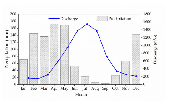
Figure 2.
The monthly dynamics of the streamflow and precipitation in the Upper Vakhsh River Basin in Central Asia (Darband station).
2.2. Data
Precipitation is the main factor in hydrological processes, as well as in hydrological modeling, while mountainous regions suffer from a lack of observational climate stations. In order to overcome this issue, most researchers are looking for an alternative option to obtain hydro-climatic data, in order to build hydrological models in mountainous watersheds and to evaluate water-balance components. Comparisons of different datasets with observational data and the combination of different datasets are appropriate objectives that have been considered here. In this study, the water-balance components were derived from the SWAT model results by applying multiple combinations of weather data products to the observational hydro-meteorological data.
Furthermore, in this study, we used the CRU Time Series (TS) version 3.1 data in our hydrological modeling of the UVRB. This data product was produced by the Climatic Research Unit at the University of East Anglia. The CRU TS 3.1 daily maximum and minimum temperatures, as well as precipitation data, were obtained from the website https://www.2w2e.com/home/CRU (accessed on 20 April 2019) for the period of 1979–2006. The reason we derived the data of CRU TS 3.1 from this site is that the historical (1970–2006) reanalysis data of precipitation and maximum and minimum temperatures from CRU TS3.1 are reformatted from NetCDF data into TXT files, which are required by SWAT. The database is updated daily, has a resolution of 0.5° and covers 67,420 files across the world’s land areas. The CRU TS 3.1 data have been used in an analysis of the historical (1970–2005) climate variability and extreme weather conditions in the state of California in the United States [41]. Touseef et al. [42] applied the CRU TS 3.1 data to validate the historical daily precipitation measurement-based data in the Xijiang River Basin in China.
The “Asian Precipitation—Highly Resolved Observational Data Integration Towards Evaluation of Water Resources Version 1101” (APHRODITE_V1101) project contains daily gridded precipitation datasets [43]. The Research Institute of Humanity and Nature and the Meteorological Research Institute of Japan’s Meteorological Agency created the APHRODITE_V1101 project by combining precipitation station data recorded from thousands of stations throughout Asia, including Japan, the Middle East, Russia, and the Asian monsoon region, to a spatial extent of 15° S–55° N, 60° E–150° E [44]. The APHRODITE_V1101 dataset is available at http://www.chikyu.ac.jp/precip/ (accessed on 6 February 2019). In the SWAT model, precipitation data alone cannot be used to build a hydrological model.
The climate forecast system reanalysis dataset (CFSR) is developed by the National Center for Environmental Prediction (NCEP) and is derived from the Global Forecast System [45]. The CFSR product is widely used in hydrological modeling, considering its high spatial resolution, robustness, and long time series. Publicly available data from January 1979 to July 2014 can be found on the official SWAT website (http://globalweather.tamu, accessed on 15 June 2019) for an almost 36-year period, in the format required by the SWAT model, for a given location. For this study, we obtained all variables of the CFSR data for 54 locations (Figure 1). Previously, many studies have been conducted to compare CFSR climate data with observational datasets to assess the reliability of gridded climate data by applying hydrological models [46,47].
The monthly discharge data for the Darband gauging station during the period of 1979–2006 in the UVRB were derived from the Department of Water Resources of the Ministry of Energy and Water Resources of the Republic of Tajikistan. The measurement-based climate data, including daily maximum and minimum temperatures and daily precipitation, were obtained from the Agency of the Hydrometeorology Committee on Environmental Protection under the Government of the Republic of Tajikistan. From the existing climate stations in Tajikistan within and outside of the UVRB, we found four climate stations, two of them within the basin—Lakhsh station in the central part of the basin, and Rasht station in the eastern part—and two more climate stations were selected from outside of the basin, Dehavz station, near to the northeastern part and Bustonobod, near to the southeastern part of the basin’s boundary.
To delineate the watershed boundary and river network of the basin, the digital elevation model (DEM) Shuttle Radar Topographic Mission (SRTM) with a 90 m (Figure 1) spatial resolution was employed, from the Consultative Group for International Agricultural Research (CGIAR) (https://www2.jpl.nasa.gov/srtm/, accessed on 16 December 2018) [48]. Soil data were obtained from the Harmonized World Soil Database (HWSD) version 1.2, with the 1:5,000,000 scale FAO/UNESCO (Food and Agriculture Organization/The United Nations Educational, Scientific and Cultural Organization) Soil Map of the World (http://www.fao.org/soils-portal/data-hub/soil-maps-and-databases/harmonized-world-soil-database-v12/en/, accessed on 29 September 2018) [49]. The area and percentage of the soil type, the latter of which is prominent in the UVRB, are shown in Table 1.
The land-use map was obtained from the Envisat Medium Resolution Imaging Spectrometer (MERIS) with a 300 300 m grid-scale. Based on the data from Envisat MERIS, the GlobCover initiative of the European Space Agency (ESA) developed and presented a service for the creation of land cover maps worldwide (https://ladsweb.modaps.eosdis.nasa.gov/missions-and-measurements/meris/, accessed on 12 September 2019) [50]. The land-use map, area, and percentage of land-use types in the UVRB are shown in Table 1. We provided five different ranges of slope classes (0–10%, 10–20%, 20–30%, 30–40%, and >40%) for the hydrologic response unit (HRU) resolution. Slope (in percent) is measured by computing the difference in the height distance (meters), divided by the lateral distance (meters), multiplied by 100. The SWAT model allowed a maximum of five ranges of slope classes. More detailed information regarding the significance of slope in hydrological modeling can be found in the studies of Yacoub et al., where the relative importance of slope discretization, compared with other discretization criteria, was assessed in the streamflow results of the SWAT model in a mountainous basin [51]. Figure 3 shows the area occupied by HRUs in the UVRB, calculated by ArcSWAT, the geographic information system (GIS) interface for SWAT.
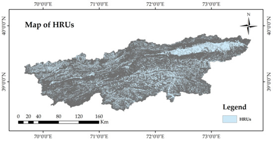
Figure 3.
The map of HRUs of the Upper Vakhsh River Basin in Central Asia. HRUs: hydrologic response units.
Figure 3.
The map of HRUs of the Upper Vakhsh River Basin in Central Asia. HRUs: hydrologic response units.

Distributed models include a large number of parameters and dealing with all these parameters at the calibration stage is not feasible. So, to ensure efficient calibration, a sensitivity analysis was conducted to filter out less influential parameters using a built-in SWAT sensitivity analysis tool. During the model calibration, the monthly observed discharge of 1979–1999 recorded at the Darband discharge station was used, which is located at the outlet of the UVRB.

Table 1.
Soil and land-use data of the Upper Vakhsh River Basin, based on area and percentage.
Table 1.
Soil and land-use data of the Upper Vakhsh River Basin, based on area and percentage.
| Land Cover Types | Area (% of Basin) | Area (km2 of Basin) | FAO Soil Name | Area (% of Basin) | Area (km2 of Basin) |
|---|---|---|---|---|---|
| Pasture | 6.57 | 1935.31 | Acrisols | 22.06 | 6495.10 |
| Agriculture | 6.58 | 1938.49 | Gleysols | 25.47 | 7499.95 |
| Forest | 1.16 | 340.38 | Leptosols | 9.17 | 2701.29 |
| Grassland | 48.63 | 14,318.06 | Phaeozems | 7.13 | 2099.55 |
| Shrubland | 4.30 | 1267.29 | Rock outcrops | 20.46 | 6024.15 |
| Urban | 0.03 | 8.07 | Eutric cambisols | 0.68 | 199.90 |
| Bare land | 16.84 | 4957.09 | Gelic gleysols | 0.02 | 7.33 |
| Water body | 0.14 | 42.08 | Glaciers | 15.00 | 4417.40 |
| Ice and snow | 15.75 | 4637.89 | |||
| Total | 100 | 29,444.66 | 100 | 29,444.66 |
3. Methodology
In this study, a physical-based, watershed-scale, continuous-time, semi-distributed hydrological model using a SWAT (soil water and assessment tool) was implemented for the evaluation of water availability in various components of the hydrological cycle in the UVRB. The United States Department of Agriculture’s Agricultural Research Service (USDA-ARS) developed the SWAT model; a detailed description of this model can be found in the theoretical documentation [52]. The SWAT model has been widely used to support water-resource managers and worldwide research dealing with water quality analyses, hydrological assessment, climate and land-use changes, water supplies, non-point-source pollution, soil erosion/sediment transport, and watershed management impact studies in small- to large-scale river basins [53]. The model does not have any limitations in terms of the river basin areas of study and is compatible with ArcGIS, QGIS, and MapWindow software, as well as providing reliable and useful theoretical documentation that is readily available. Using the ArcGIS version 10.3 interface of SWAT, named ArcSWAT, the UVRB was divided into sub-basins, based on a digital elevation model. Each sub-basin is connected through a stream channel and the model operates by dividing sub-basins into many HRUs (Figure 3), according to a unique homogenous combination of land cover, soil properties, and terrain features. The model performs a modification of the soil conservation service curve number (SCS-CN) method, which identifies the surface runoff from daily precipitation, land use, the area of the hydrological group and the antecedent moisture content for each HRU [54,55].
The UVRB is a mountainous catchment; hence, the observational climate stations in the UVRB are located at lower altitudes. For instance, the Rasht station is located at an elevation of 1316 m, Bustonobod at an elevation of 1964 m, Lakhsh at an elevation of 1998 m, and Dehavz at an elevation of 2561 m. The orographic features of the UVRB mountainous catchment, in terms of temperature and precipitation, led to the splitting of the UVRB into different elevation bands in the SWAT model. In order to simulate the snowmelt in this study, we used a temperature index algorithm employing the elevation band approach [56,57]. We weighted the temperature and precipitation elevation band between the climatic station band and the other elevation band (EB) by using the following mathematical equations:
where 1000 serves as the conversion element from meters to kilometers; is the precipitation in an EB (mm); is the precipitation recorded at the measurement gauge (mm); shows the daily maximum temperature of the EB (; indicates the daily minimum temperature of the EB (; is the daily mean temperature of the (; shows the daily maximum temperature recorded at the measurement gauge (; indicates the daily minimum temperature recorded at the measurement gauge (; shows the daily average temperature recorded at the measurement gauge (; is the lapse rate of temperature ( shows the mean elevation in the EB (m); indicates the elevation at the measurement gauge (m); is the precipitation lapse rate (mm/km) and represents the average annual value of the days when precipitation occurred. The EB approach to the SWAT model has been employed in various mountainous catchments across the globe [58,59,60]. As in our previous study, Gulakhmadov et al. presented the hydrological model calibration results they obtained with the SWAT–CUP tool before and after the EB approach. The application of EB had a positive impact on the modeling of river flow in a mountain watershed [61].
The model was auto-calibrated for sensitive parameters, such as runoff curve number (CN), Manning’s n, and groundwater (GW) parameters (Soil K, Ch_K, Alpha BF, REVAP, ESCO, soil AWC, GW delay, Recharge_DP, Soil Z), based on their rankings. A multiple regression equation was used to identify the sensitive parameters, as follows:
where shows the value of the objective function; indicates the parameter of the calibration; and represent the regression coefficients; and m indicates the selected parameter number [62].
The simulation of the hydrological processes by SWAT is carried out on the basis of the water balance equation:
where shows the initial soil water content on day (mm H2O); is time in days; shows the amount of precipitation on day (mm H2O); is the amount of surface runoff on day (mm H2O); is the amount of evapotranspiration (ET) on day (mm H2O); is the amount of water entering the vadose zone from the soil profile on day (mm H2O); is the amount of return flow on day (mm H2O); and shows the final soil water content (mm H2O).
On the basis of the average daily air temperature, the SWAT model divides the precipitation into rain or snow. The user of the model will give a threshold temperature in order to categorize precipitation as rain or snow. The precipitation, as snow, will be modeled and the equivalent water will be supplemented to the snowpack if the average air temperature is lower than the temperature threshold. The precipitation will be modeled in the form of liquid rain if the average daily temperature is higher than the temperature threshold. If additional snow falls, the snowpack will be raised and if snowmelt or sublimation occur, the snowpack will be reduced, and the water accumulation in the snowpack will be given as the snow water component.
The SWAT model calculates the snowmelt as a linear function of the divergence between the mean maximum temperature of the snowpack and the snowmelt threshold temperature or base. The snowmelt on a given day is calculated based on the following equation:
where represents the melt factor for the day (mm H2O/day-°C); the fraction of the HRU area covered by snow is ; the temperature of the snowpack is (°C); the maximum air temperature is ; the base temperature above which snowmelt is allowed is (°C); and indicates the amount of snowmelt (mm). Seasonal differences are allowed by the melt factor, with maximum and minimum indices, taking place towards winter and summer solstices:
where represents the melt factor for 21 June (mm H2O/day-°C); the melt factor for 21 December is (mm H2O/day-°C); is the day of the year, and the resulting value () shows the melt factor for the day (mm H2O/day-°C).
The evaluation of evapotranspiration (ET) is essential for water-resource management and hydrological research. The studies of previous researchers suggested that it is acceptable to apply PET (potential evapotranspiration) in models and water allocations [63,64]. In order to estimate PET, there are three methods given in the SWAT model, including the radiation-based Priestley and Taylor method [65], the temperature-based Hargreaves method [66], and the combined Penman–Monteith method [67,68]. For the present study, the Hargreaves method depends on inputted climate data, which were selected to determine the potential evapotranspiration in a mountainous catchment. The Hargreaves approach is the most commonly used method; it is based on temperature and is recommended by the FAO. Li et al. compared the results of the Hargreaves and Penman–Monteith methods in the Ganjiang River Basin in Southern China by using two different datasets [69]. The results of the analysis showed that there is no significant discrepancy between the Hargreaves and Penman-Monteith methods in terms of streamflow simulations with the same spatial scale. The ET was computed as a function of the corrected potential evapotranspiration, soil depth, soil cover, and plants’ water uptake [52]. Based on each hydrological response unit, the water balance components were simulated, including precipitation partitioning, precipitation interception, evapotranspiration, snowmelt water, the redistribution of soil water content, return flow from shallow aquifers and lateral subsurface flow from the soil profile.
Model Assessment
The model evaluation was carried out based on the Nash–Sutcliffe efficiency (NSE) measure, the coefficient of determination (R2), and the percentage bias (PBIAS). Model assessment statistics were evaluated using the NSE, R2, and Kling–Gupta efficiency (KGE) calculations [70]. In watershed modeling, the NSE, R2 and KGE are standard regression statistics [71]. NSE ranges from −∞ to 1, with 1 being the best performance. The degree of the linear relationship between measured data and model output is R2 and it ranges between 0 and 1. KGE is the goodness-of-fit measure initiated by Gupta et al. [70], which gives a decomposition of mean squared error and NSE. In hydrological modeling, the KGE statistic value contributes to the analysis of the relative significance of the correlation, variation, and bias [72]. The model result is more accurate if the KGE output value is closer to 1, and it ranges from −∞ to 1. Moreover, in the model performance, we used the root mean square error (RMSE) observed standard deviation ratio (RSR) and an error-index statistic. The values of NSE > 0.50 and R2 > 0.60 are considered satisfactory for river discharge on a monthly scale [71]. The values of KGE > 0.5 and RSR < 0.60 are also considered satisfactory levels [70,71]. To assess the strength of the model calibration and uncertainty, two important factors were computed based on the calibration of soil and water assessment tool model (SWAT–CUP) performance, the P-factor and R-factor [73,74]. According to Abbaspour et al. [74], the P-factor describes the percentage of observational data that is covered with a 95% prediction uncertainty (95PPU). It quantifies the model’s capability in terms of catching uncertainties, and its magnitude ranges between 0 and 1, where 1 demonstrates that 100% of the station-recorded variability is captured by 95PPU. The thickness of 95PPU is the value of the R-factor, which presents the ratio of the mean width of the 95PPU band and the standard deviation of measured variability. The model performance is superior if the R-factor value is low. For discharge modeling, in order to compute prediction uncertainty, the studies of Abbaspour et al. [74] recommended that the value of the P-factor be > 0.7 and the value of the R-factor be < 1.5.
The NSE, the R2, the PBIAS, the RSR, KGE, and MSE are frequently applied measures in hydrological modeling studies [71], which are calculated as:
where n is the whole number of sample couples; is the station-recorded discharge variable; is the mean of the station-recorded discharge parameters; is the simulated discharge parameter; is the mean of the simulated discharge parameters; and is the th station-recorded data or simulated data. Moreover, and , while is the linear regression coefficient of the simulated value against station-recorded value, and are the averages of the simulated value against the station-recorded value, and and are the standard deviations of the simulated value against the station-recorded value [70].
4. Results
In hydrological process analysis, and for reliable hydrological modeling, precipitation data are considered to be the main factor. To apply the precipitation data initially in hydrological modeling, we carried out a correlation analysis to examine the data’s suitability for watershed modeling. Figure 4 presents a Taylor diagram with the performances of the three precipitation data sources, the CRU TS3.1, CFSR and APHRODITE_V1101, against measurement-based precipitation data on a monthly scale. Taylor diagrams are capable of providing performance insights by comparing precipitation satellite datasets and measurement-based data sets, in terms of their standard deviation, root mean square error and correlation coefficient. In the Taylor diagram, the radial blue dotted lines show the standard deviation and the red semicircles present the root mean square error. Hence, the black dotted lines describe the correlation coefficient. These three statistic indices are shown solely for the Lakhsh precipitation gauge point in the central part of the catchment on a monthly scale, for the purposes of demonstration (Figure 4). The precipitation correlation showed the highest value (0.86) between the APHRODITE_V1101 datasets and measurement-based datasets. Meanwhile, the precipitation correlation between the CRU TS3.1 and measurement-based data is 0.76, and the correlation between the CFSR and measurement-based datasets is 0.59. The correlation coefficients between all three different combinations, the CRU TS3.1 and measurement-based datasets, CFSR and measurement-based datasets, as well as APHRODITE_ V1101 and measurement-based datasets, showed a good performance, meaning that they could be used for hydrological modeling in the UVRB. In many studies, Taylor diagrams have been applied to evaluate the performance of satellite products against observational datasets [75,76].
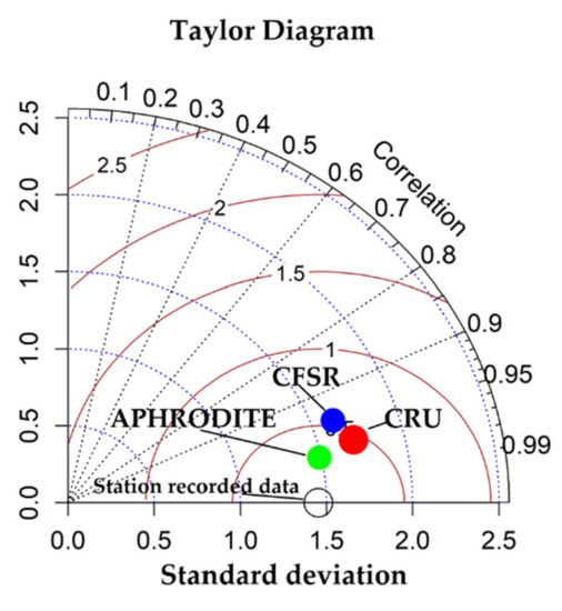
Figure 4.
Taylor diagram indicating the performances of CRU, CFSR and APHRODITE precipitation data on a monthly scale at the Lakhsh climate station in the Upper Vakhsh River Basin in Central Asia.
4.1. Parameter Sensitivity Analysis
The hydrological model was calibrated and validated by employing a software application for the SWAT–CUP, SUFI-2 (sequential uncertainty fitting, version 2). The SWAT–CUP software is a semi-automatic calibration and uncertainty analysis tool that was developed by the EAWAG Swiss Federal Institute of Aquatic Science and Technology for the SWAT model [3]. The SUFI-2 algorithm utilizes an inversion modeling technique that determines a wide range of parameters and then carries out several iterations that contain a number of simulations. After running the iterations, the result of each iteration was compared with the result of other iterations and, in this way, the most suitable ranges of the model’s parameters were identified [74]. This iterative procedure takes into account the uncertainty of parameters from all types of sources, including model structure, model parameters, weather, etc. By using the global sensitivity approach in the SUFI-2 algorithm, detailed uncertainty and optimization examinations are possible [77]. In order to obtain satisfactory watershed characteristics, the calibration and validation of the hydrological model are essential. Following the outcome of the final modeled simulation, a sensitivity ranking was presented for the appropriate parameters by analyzing the values of the “t-stat” and p-value statistics. The SWAT–CUP contains multiple parameters that could impact the simulation of the water cycle. The selection of suitable parameters plays an important role in identifying the effectiveness of model calibration.
In this study, the sensitivity analysis was executed using the Latin hypercube global sensitivity approach, which is included in the SWAT–CUP (version 2019) package. Characteristically, sensitivity analysis is required prior to calibration due to the recognition of sensitive parameters and model elements. The global sensitivity approach leads to the attainment of a set calibration with optimal parameters and allows us to find the parameters using the degree of sensitivity of their performance characteristics in the model.
A gridded dataset comparison was performed to evaluate how well gridded datasets, such as CRU TS3.1, APHRODITE_V1101 and CFSR, correlated with the observational data. The analysis years were determined to include similar years from all datasets since CRU daily data availability ended in 2006. The first three years of the total simulation period (January 1999–December 2002) were used as a warm-up to allow the model to reach hydrological equilibrium and were excluded from the analysis. For each of the datasets, the semi-automated calibration process was conducted with an identical range of parameter values and calibration/validation periods for comparison purposes. Semi-automated calibration ensures the consistency of the process for all models, minimizing the model bias due to the modeler in calibration exercises conducted for different precipitation and maximum/minimum temperature sources. Initial parameter ranges were selected based on the professional judgment of the authors and the literature. Each model executed 1000 simulations for each iteration of the semi-automated calibration. An initial 300–500 simulations are recommended for studying model performance and for regionalizing parameters [73]. At the end of the iteration with 1000 simulations, parameter sensitivities were determined through a global sensitivity analysis. Only one iteration was used to avoid re-calibration, using a different range of parameter values for each model in the subsequent calibration. The Nash–Sutcliffe efficiency (NSE) measure was used to estimate model performance during calibration since it is a commonly used statistical measure in SWAT studies [71].
While determining the parameters’ distribution and sensitivity, the baseflow alpha factor (ALPHA_BF), moist bulk density (SOL_BD), SCS runoff curve number for moisture condition II (CN2), effective hydraulic conductivity in main channel alluvium (CH_K2), and deep aquifer percolation fraction (RCHRG_DP) are computed as the most sensitive parameters. The results of sensitivity parameters and analyses of statistical indices, such as P-factor and R-factor, in both calibration and validation parts indicated that all climate datasets utilized in this study have acceptable prediction uncertainty and reasonable parameter adjustment. These results indicate the potential of applying gridded datasets for hydrological modeling. It should be noted that gridded datasets are advantageous because they give continuous data at spatial and temporal scales throughout the catchment area and for an extensive duration.
4.2. Calibration and Validation
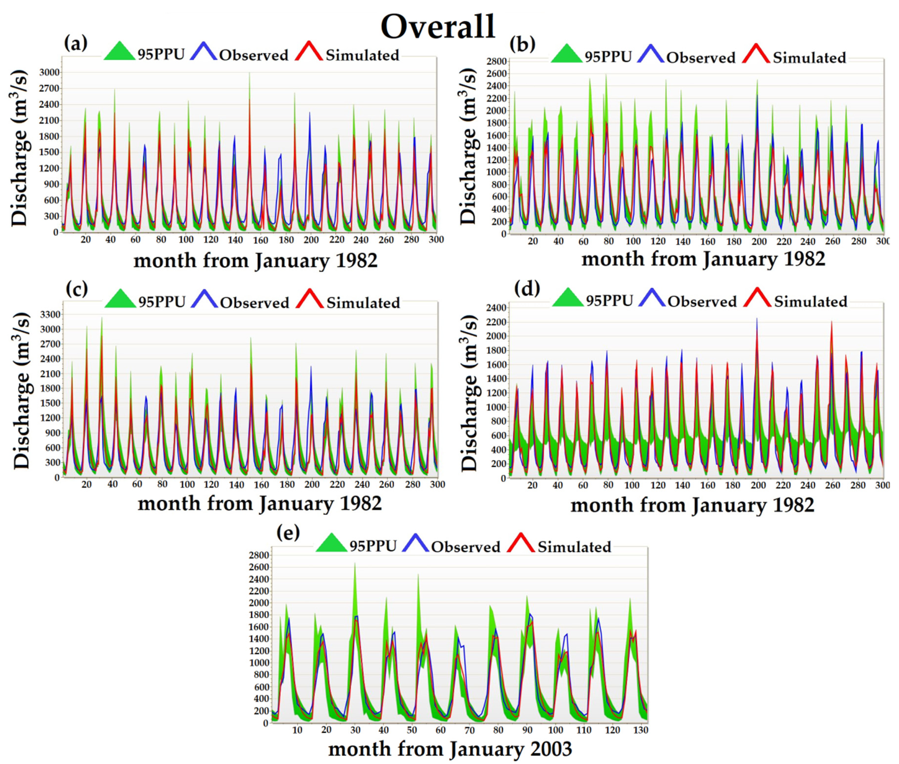
Figure 5 shows the calibration results of the SUFI-2 algorithm of the SWAT–CUP model, utilizing monthly discharge data at the Darband gauging station for the period of 1982–1999, where a combination of four different datasets was used (Figure 5a–d), including an initial warm-up period of three years (1979–1981). Figure 6 indicates the validation results of the fit between the monthly measurement-based flow and the flow simulated by SWAT. In addition, to demonstrate the flow peaks over a long period of time, in Figure 7, we present the overall calibration hydrographs via the application of five different dataset combinations.
Table 2 shows the ability of gridded datasets to derive the long-term average annual flow from the simulated flow at the Darband gauging site in UVRB in Central Asia. The observation and simulated flow over a 25-year period demonstrated that the average annual flow between the observation and the simulated flow does not differ much, with the exception of a few years. The results shown as Simulated-1 in Table 2 demonstrate that, in most years, the average annual flow was simulated to be less, compared to the other three simulated flows. In Simulated-1, the largest negative ratio value between the observed and simulated average annual flows was found in 1996 (−123.87%) and 1988 (−124.79%), while the largest positive value of the ratio was observed in 1983 (13.58%). The results of Simulated-2 presented the lowest negative ratio value of the average annual flow in 2006 (−59.79%) and the highest positive value in 1989 (35.69%). The maximum negative and positive rates of the average annual flow for Simulated-3 were detected in 1984 (27.66%) and 1998 (−74.62%), while for Simulated-4, the biggest downward and upward rate values compared to observational flow were obtained in 1997 (−42.27%) and 2003 (26.53%). Our results show that, compared with the observational average annual flow, the average annual flow of Simulated-1 indicated the largest negative rate, and the Simulated-4 results showed the lowest negative and positive rates (Table 2). In this study, the four different quantity comparisons of the average annual flow were derived after the application of a well-calibrated hydrological model.
Table 2.
Average annual simulated flow of four different simulation results from SWAT–CUP and their rates, compared to observational flow at the Darband hydrological station over the period of 1982–2006 in the Upper Vakhsh River Basin in Central Asia. Simulated-1: results of the combination of the APHRODITE_V1101 precipitation datasets and CFSR maximum/minimum temperature datasets; Simulated-2: results of the combination of the APHRODITE_V1101 precipitation datasets and CRU TS3.1 maximum/minimum temperatures datasets; Simulated-3: results of the CFSR as maximum/minimum temperatures, precipitation, average solar radiation, average wind speed and relative humidity datasets; Simulated-4: results of the CRU ST3.1 precipitation and maximum/minimum temperature datasets.
The observed and simulated monthly streamflow values for the calibration (1982–1999), validation (2000–2006), and overall values (1982–2006) are shown in Figure 5, Figure 6 and Figure 7, respectively. Figure 5, Figure 6 and Figure 7 present the simulated flow hydrographs and peak flows, which are in good agreement with the timing of the observational flow hydrographs and flow peaks comprising the outcomes of the APHRODITE_V1101 and CFSR combination, the APHRODITE_V1101 and CRU TS3.1 combination, and the CRU TS3.1, CFSR, and measurement-based combination. Calibration using monthly river flow data for long-term simulations demonstrates a better performance than short-term simulations. The base flow as well as most of the peak flows are well simulated. The hydrographic results show that the observed and modeled discharges are nearly the same for most of the study period (25 years), except for a few years when high-flow events occurred. For example, the peak flow in the hydrograph for the combination of APHRODITE_V1101 and CFSR in 1987, 1993, 1996, and 1998 is underestimated by the model, while in the years 1984 and 1994 it is overestimated (Figure 7a). The peak flow rate for the combination of APHRODITE_V1101 and CRU TS3.1 in 1989, 1991 and 1997 is insignificantly underestimated (Figure 7b). The model insignificantly underestimated the peak flow for the CFSR dataset in the years 1987, 1989, 1996 and 1998, while in the years 1983, 1984, 1994 and 2001, it slightly overestimated the flow (Figure 7c). For the CRU TS3.1 hydrograph, a slight underestimation of the peak flow is observed in the years 1983, 1987, 2000 and 2001, whereas in the year 2003, the flow is slightly overestimated (Figure 7d). Lastly, the model insignificantly underestimated the peak discharges in 2008 and 2011 for the observational datasets (Figure 7e). Our results showed that better simulation flows were obtained from APHRODITE_V1101 and CRU TS3.1 climate datasets compared to the CFSR, which demonstrates the advantage of using the CRU TS3.1 and APHRODITE_V1101 products in SWAT modeling.
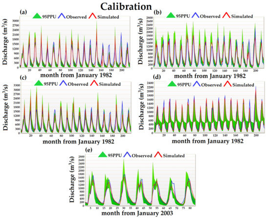
Figure 5.
Hydrographic calibration between monthly observed and simulated streamflow, when applying the SWAT–CUP tool, at Darband gauging station in the Upper Vakhsh River Basin in Central Asia. (a) Results of the daily precipitation of the APHRODITE_V1101 and daily maximum/minimum temperatures from the CFSR datasets; (b) results of the daily precipitation of the APHRODITE_V1101 and daily maximum/minimum temperatures of the CRU TS3.1 product; (c) results of the daily maximum/minimum temperatures, precipitation, average solar radiation, average wind speed and relative humidity from the CFSR product; (d) results of the daily maximum/minimum temperatures, and precipitation from the CRU TS3.1 product; (e) results of the daily maximum/minimum temperatures and precipitation from the observational climate datasets.
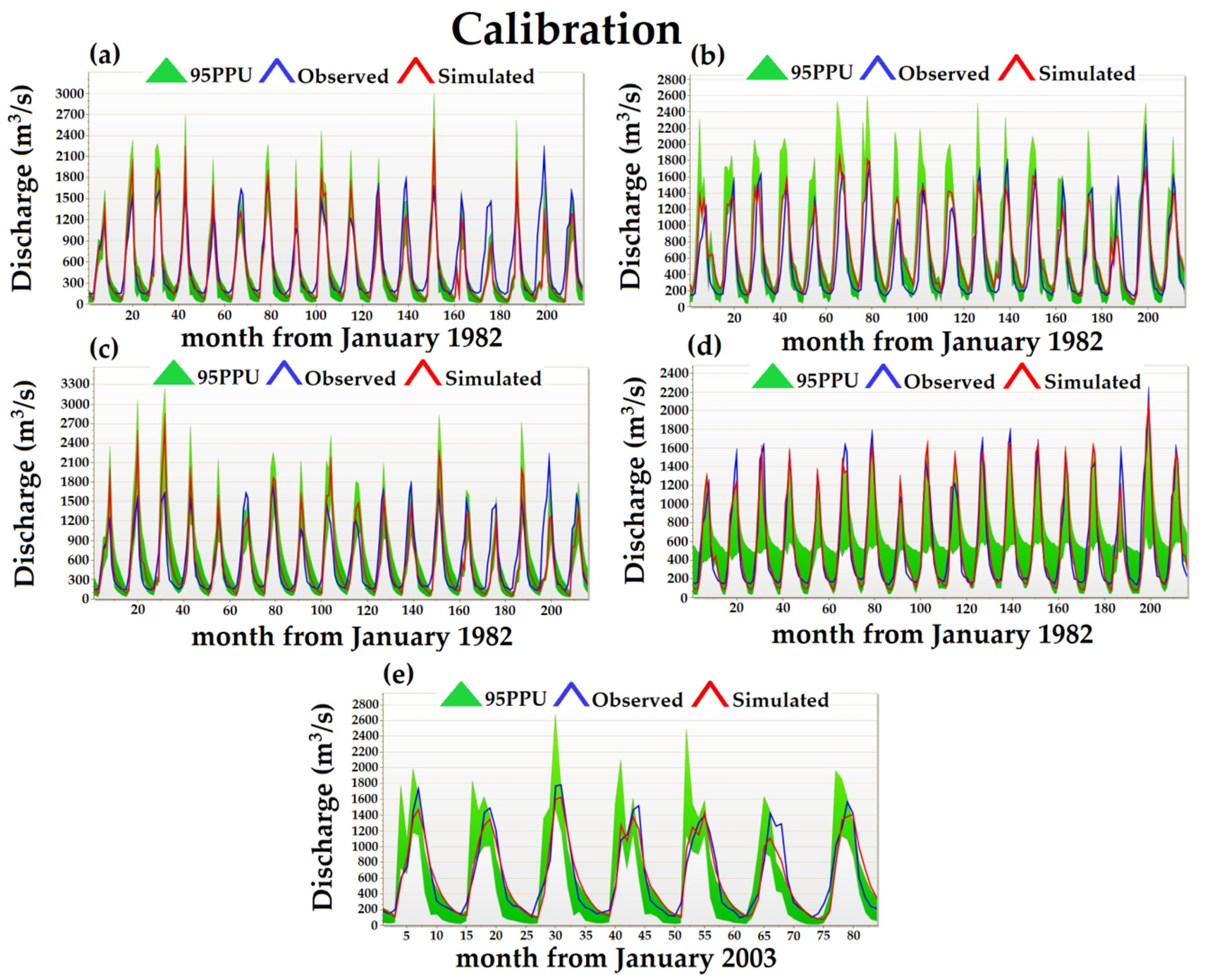

Figure 6.
Hydrographic validation between monthly observed and simulated streamflow, when applying the SWAT–CUP tool, at Darband gauging station in the Upper Vakhsh River Basin in Central Asia. (a) Results of the daily precipitation of the APHRODITE_V1101 and daily maximum/minimum temperatures from the CFSR datasets; (b) results of the daily precipitation of the APHRODITE_V1101 and daily maximum/minimum temperatures of the CRU TS3.1 product; (c) results of the daily maximum/minimum temperatures, precipitation, average solar radiation, average wind speed and relative humidity from the CFSR product; (d) results of the daily maximum/minimum temperatures, precipitation from the CRU TS3.1 product; (e) results of the daily maximum/minimum temperatures and precipitation from the observational climate datasets.
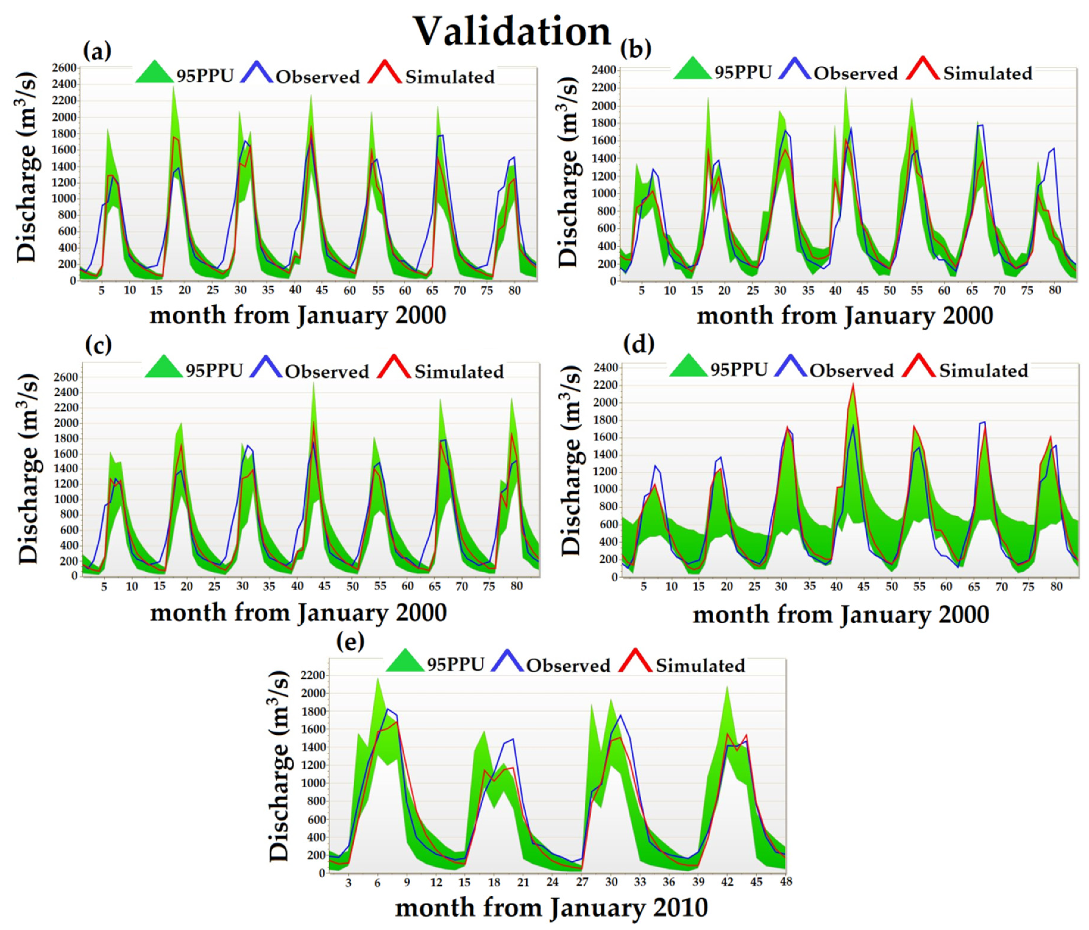

Figure 7.
Hydrograph of the overall calibration and validation period between monthly observed and simulated streamflow, when applying the SWAT–CUP tool, at Darband gauging station in the Upper Vakhsh River Basin in Central Asia. (a) Results of the daily precipitation of the APHRODITE_V1101 and daily maximum/minimum temperatures from the CFSR datasets; (b) results of the daily precipitation of the APHRODITE_V1101 and daily maximum/minimum temperatures of the CRU TS3.1 product; (c) results of the daily maximum/minimum temperatures, precipitation, average solar radiation, average wind speed and relative humidity from the CFSR product; (d) results of the daily maximum/minimum temperatures, precipitation from the CRU TS3.1 product; (e) results of the daily maximum/minimum temperatures and precipitation from the observational climate datasets.
4.3. Performance of the Hydrological Model
Table 3, which presents the statistical values for the calibration, validation and overall periods of the Darband discharge station, confirms the essentially “excellent”, “very good” and “good” performance of the model. Firstly, in the SUFI-2 algorithm, we adopted the Nash–Sutcliffe efficiency (NSE) calculation as an objective function for the optimization process. It was used as a goodness-of-fit metric for calibration, in order to set up the adjustment during the calibration period and for the performance examination of the validation and overall periods. The NSE working system has been recognized for its ability to concentrate on the good simulation of peak flows. Its selection and related influence should be considered in view of the results obtained in this study. A more general view, which included all modeling on an overall scale for all datasets, showed that most of the years provided accurate modeling in all angles of the hydrograph.
In general, eight kinds of evaluation indices (R2, NSE, PBIAS, RSR, MSE, KGE, P-factor and R-factor) were used to evaluate the acquisition accuracy of the hydrological modeling. The statistical evaluation of the model performance based on monthly streamflow is described in Table 3. The streamflow is slightly overestimated by 14.8%, 1.32% and 0.69% for the APHRODITE_V1101+CFSR, CRU TS3.1 and measurement-based data while being slightly underestimated by −17.70% and −0.31% for APHRODITE_V1101+CRU TS3.1 and CFSR during the calibration period. During the validation period, the model results for the employed APHRODITE_V1101+CFSR, APHRODITE_V1101+CRU TS3.1, CFSR and observational datasets indicated an overestimation of the monthly streamflow by 17.22%, 1.3%, 9.58% and 5.51%, respectively, while the model results showed an underestimation by −6.09% for the CRU TS.3.1. The model results of the overall test performance of the calibration indicated an overestimation of the peak flow for the APHRODITE_V1101+CFSR, CFSR, CRU TS3.1, and observational data by 15%, 2%, 0.29% and 5.21% respectively, whereas, for the APHRODITE_V1101+CRU TS3.1, the results showed an underestimation of peak flow by −10.80% (Table 2). However, the combination of the precipitation data from APHRODITE_V101 and the maximum/minimum temperatures data from CFSR exhibited a slightly overestimated streamflow, which can probably be explained by the large amount of precipitation generated by APHRODITE_V1101. As we realized that precipitation is a major factor in hydrological processes, and in an effort to demonstrate the difference in precipitation between the four climate datasets, before implementing the data into the model, we correlated the precipitation between the observational data and APHRODITE_V1101, CFSR, and CRU TS3.1, as presented in Figure 4. In general, for calibration and validation periods, the hydrographs of all utilized datasets are nearly in line with measurement-based data. According to the recommendation of Moriasi et al. [71], the performance of the model is “very good” (PBIAS 10) in the study area, based on four different combinations of datasets.
In the case of monthly calibration, validation and overall scales, the P-factor ranges from 0.66 to 0.82 for all employed datasets. By using the APHRODITE_V1101+CFSR, APHRODITE+CRU TS3.1, CFSR, CRU TS3.1 and observational values, the bracketed values of the 95PPU band for the monthly streamflow data were 66%, 66%, 75%, 82% and 69% during the calibration period, 67%, 70%, 79%, 80% and 81% during the validation period and 66%, 68%, 75%, 81% and 73% on an overall scale, respectively. The R-factor is the average thickness of the 95PPU band, and, for the monthly calibration, validation and overall scales, the R-factor values were 0.66, 0.79, 0.95, 1.01, and 0.80 (calibration), 0.66, 0.66, 0.89, 1.08, and 0.76 (validation), and 0.67, 0.75, 0.95, 1.02, and 0.78 (overall) when coupling the SWAT model with the respective datasets. The wider 95PPU indicates more parameter uncertainties [62]. According to the recommendations of Schuol et al. [78], the perfect simulation is the one that has an R-factor equal to zero; however, values around 1.0 are considered quite reasonable. In this study, the values obtained for the width of the uncertainty band were quite reasonable for the monthly simulation (Table 3).
The model results for the calibration, validation and overall periods were found to produce a reliable assessment of monthly observed and simulated streamflow. The monthly calibration results for streamflow were “very good”, with R2 values of 0.92, 0.90, 0.79, and 0.76 for the CRU TS.3.1, measurement-based, APHRODITE_V1101+CRU TS3.1, and APHRODITE_V1101+CFSR data, whereas for CFSR, the data were found to possess a “good” performance, with an R2 value of 0.71. The NSE values were “very good” at 0.91 and 0.90 for CRU TS3.1 and observational datasets, “good”, at nd , for APHRODITE_V1101+CRU TS.3.1 and APHRODITE_V1101+CFSR, and “satisfactory” at for CFSR during the calibration period. The R2 and NSE coefficient values during the validation period were “very good” (R2 equal to 0.94, 0.89, 0.85, 0.83, and 0.79 and NSE equal to 0.93, 0.88, 0.83, 0.77, and 0.78) for the observational datasets, CRU TS3.1, CFSR, APHRODITE_V1101+CFSR and APHRODITE_V1101+CRU TS3.1, respectively. This is likely due to the availability of data and the mountainous location of the precipitation station in this region, since the distribution of precipitation strongly influences the flow formation and therefore the NSE. The overall R2 coefficient values were “very good” (0.92, 0.90, 0.78, and 0.76 for the observational datasets, CRU TS3.1, APHRODITE_V1101+CFSR, and APHRODITE_V1101), whereas R2 was “good” (0.74 for the CFSR (Table 3)). The overall NSE coefficient values were “very good” (0.91 and 0.90 for the observational datasets and CRU TS3.1), while the NSE values were “good” (0.74, 0.72, and 0.68 for the APHRODITE_V1101+CRU TS.3.1, APHRODITE_V1101+CFSR, and CFSR, respectively). According to the model evaluation criteria, the simulation of the observational data performed better than the APHRODITE_V1101+CFSR, APHRODITE_V1101+CRU TS.3.1, CFSR and CRU TS3.1 simulations on an overall scale. The model using observational dataset calibration, validation, and overall scales demonstrated an excellent performance (Table 3). The less accurate results that were obtained overall, when using gridded datasets in mountainous regions, are most probably associated with the fact that there are fewer weather stations that can be used for product development.
Table 3.
Summary statistical indices of monthly streamflow periods with different climate datasets, based on the model’s performance. NSE: Nash–Sutcliffe efficiency; R2: coefficient of determination; PBIAS: percentage bias; MSE: mean square error; RSR: root mean square error standard deviation ratio; KGE: Kling–Gupta efficiency; P-factor; R-factor.
| Data Source\Statistical Indices | R2 | NSE | PBIAS (%) | RSR | MSE (%) | KGE | P-Factor | R-Factor |
|---|---|---|---|---|---|---|---|---|
| Calibration | ||||||||
| Combination of the APHRODITE_V1101 and CFSR data (1982–1999) | 0.76 | 0.70 | 14.80 | 0.55 | 7.78 | 0.80 | 0.66 | 0.66 |
| Combination of the APHRODITE_V1101 and CRU TS3.1 data (1982–1999) | 0.79 | 0.74 | −17.70 | 0.77 | 6.72 | 0.77 | 0.66 | 0.79 |
| CFSR data (1982–1999) | 0.71 | 0.64 | −0.31 | 0.60 | 9.12 | 0.81 | 0.75 | 0.95 |
| CRU TS3.1 data (1982–1999) | 0.92 | 0.91 | 1.32 | 0.29 | 2.23 | 0.95 | 0.82 | 1.01 |
| Observational data (2003–2009) | 0.90 | 0.90 | 0.69 | 0.31 | 2.54 | 0.90 | 0.69 | 0.80 |
| Data source | Validation | |||||||
| Combination of the APHRODITE_V1101 and CFSR data (2000–2006) | 0.83 | 0.77 | 17.22 | 0.48 | 6.01 | 0.81 | 0.67 | 0.66 |
| Combination of the APHRODITE_V1101 and CRU TS3.1 data (2000–2006) | 0.79 | 0.78 | 1.30 | 0.46 | 5.54 | 0.80 | 0.70 | 0.66 |
| CFSR data (2000–2006) | 0.85 | 0.83 | 9.58 | 0.42 | 4.48 | 0.87 | 0.79 | 0.89 |
| CRU TS3.1 data (2000–2006) | 0.89 | 0.88 | −6.09 | 0.35 | 3.18 | 0.91 | 0.80 | 1.08 |
| Observational data (2010–2013) | 0.94 | 0.93 | 5.51 | 0.26 | 2.04 | 0.93 | 0.81 | 0.76 |
| Data source | Overall | |||||||
| Combination of the APHRODITE_V1101 and CFSR data (1982–2006) | 0.78 | 0.72 | 15.00 | 0.53 | 7.20 | 0.81 | 0.66 | 0.67 |
| Combination of the APHRODITE_V1101 and CRU TS3.1 data (1982–2006) | 0.76 | 0.74 | −10.80 | 0.51 | 6.70 | 0.78 | 0.68 | 0.75 |
| CFSR data (1982–2006) | 0.74 | 0.68 | 2.00 | 0.56 | 8.10 | 0.83 | 0.75 | 0.95 |
| CRU TS3.1 data (1982–2006) | 0.90 | 0.90 | 0.29 | 0.31 | 2.51 | 0.95 | 0.81 | 1.02 |
| Observational data (2003–2013) | 0.92 | 0.91 | 5.21 | 0.29 | 2.34 | 0.93 | 0.73 | 0.78 |
4.4. Water Balance of the Upper Vakhsh River Basin in Central Asia
Obviously, in order to skillfully tackle water management issues, it is necessary to quantify and study the various hydrological components within the basin. Regardless of the issues explored by the SWAT model, water balance is a critical component in the SWAT model as it includes all processes in the basin [79,80]. A water-balance study was conducted using a simulation of the overall scale, as well as the appropriate SWAT output tables. The mean annual water-balance components of the UVRB are presented in Table 4.
Table 4.
The mean annual water balance components of the Upper Vakhsh River Basin in Central Asia during the calibration (1982–1999), validation (2000–2006) and overall (1982–2006) periods generated from the SWAT model. (a) Combination of the APHRODITE_V1101 and CFSR datasets; (b) combination of the APHRODITE_V1101 and CRU TS3.1 datasets; (c) CFSR data source; (d) CRU TS3.1 datasets; and (e) observational datasets.
The results of the SWAT model for the overall period of the simulation (1982–2006) are presented; the annual precipitation values for the basin are 1875.9 mm, 1236.9 mm, 2479 mm, 1215.9 mm, and 1098.5 mm, out of which about 93.82% (1760.11 mm), 70.41% (870.85 mm), 96% (2379.86 mm), 86.52% (1051.98 mm), and 76.16% (836.65 mm) of precipitation falls as snow, according to the respective datasets employed (Table 4). The CFSR simulations demonstrated a higher amount of precipitation than other utilized, which means that the CFSR overestimated the precipitation in the UVRB. Similarly, Hu et al. [81] reported an overestimation in the results of the CFSR precipitation datasets used in a mountainous region of Central Asia. Mean annual evapotranspiration from the whole catchment is about 9.93%, 25.52%, 2.9%, 21.08%, and 27.28% of the annual precipitation (186.3 mm, 315.7 mm, 72.1 mm, 256.4 mm, and 299.7 mm out of 1875.9 mm, 1236.9 mm, 2479 mm, 1215.9 mm, and 1098.5 mm) when using the respective datasets. Water yield is as streamflow, which is obtainable at the catchment outlet and is determined from surface runoff, lateral flow and baseflow or return flow. Based on the respective datasets on an overall scale, the annual water yields at the catchment outlet are 534.72 mm, 771.24 mm, 661.98 mm, 672.11 mm, and 654.97 mm, from which surface runoff or overland flow can be obtained; these take place across a sloping surface at about 46.54 mm, 276.79 mm, 90.56 mm, 30.73 mm, and 243.22 mm (including channel losses). The lateral subsurface flow or interflow, which originates below the surface but above the rock saturation zone, contribute 413.34 mm, 371.49 mm, 331.92 mm, 394.21 mm, and 307.92 mm (about 77.30%, 48.17%, 50.14%, 58.65%, and 47.01% of the total water yield) to all aforementioned combinations of datasets. The remaining flow is contributed by the base flow, which originates from groundwater (shallow aquifer). The annual mean streamflow during the period of 1979–2006 at the Darband discharge station at the outlet point of the UVRB is 626.08 m3/s. The threshold depth of water in the shallow aquifer (REVAP) takes into account the volume of water transported from a shallow aquifer to overlying unsaturated terrain during the dry season.
The mean monthly values of precipitation, water yield, and actual evapotranspiration for the UVRB are also estimated by coupling the combination of the respective datasets, as demonstrated in Figure 8. The low precipitation period occurs in July, August and September, while May–September is the high flow period and flow is less affected by precipitation events during this time. Similarly, evapotranspiration is higher from May to September and the large runoff over this period is mainly due to the melting of the snowpack and permanent glaciers. Moderately high and high precipitation occurs from October to June. In this study, the maximum precipitation values of 227.21 mm, 154.87 mm, 279.76 mm, 153.29 mm, and 135.54 mm per month occurred in May, according to the respective datasets. Based on the CRU TS3.1 and observational datasets, July and August are the only months where actual evapotranspiration is higher than total precipitation during the dry period. This may have happened because evapotranspiration is a sustained process that takes place during the day and night. The simulation of all employed datasets revealed that the maximum evapotranspiration occurred in July. The higher mean monthly actual evapotranspiration generated the simulation of the observational datasets, while the CFSR simulation produced lower than average actual evapotranspiration in all months compared to other simulated datasets for the entire catchment. The CRU TS3.1 dataset simulations and the APHRODITE_V1101+CRU TS3.1 simulations of the mean monthly actual evapotranspiration showed a “very good” correlation with the observational dataset simulations. For example, about 70% of the evapotranspiration occurred from May to August and, during this period, the APHRODITE_V1101+CRU TS3.1 datasets simulated about 39.86 mm, 55.01 mm, 62.70 mm, and 49.27 mm, the CRU S3.1 datasets simulated about 36.36 mm, 50.63 mm, 55.02 mm, and 33.93 mm, and the observational datasets simulated about 42.95 mm, 56.69 mm, 60.19 mm, and 48.05 mm of evapotranspiration.

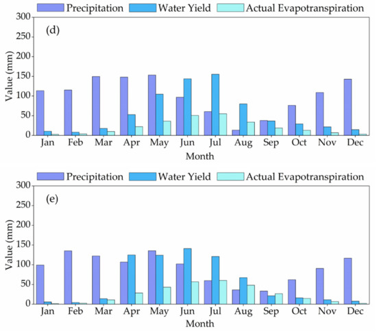
Figure 8.
Mean monthly basin values of precipitation, water yield and actual evapotranspiration in the Upper Vakhsh River Basin in Central Asia, using (a) APHRODITE_V1101+CFSR, (b) APHRODITE_V1101+CRU TS3.1, (c) CFSR, (d) CRU TS3.1, and (e) observational datasets.
The mean annual values of precipitation for the UVRB are also estimated using the SWAT model by coupling the combination of the respective datasets, as demonstrated in Table 4. Due to the combination of the different dimensions of the gridded datasets, the SWAT model results showed mean annual precipitation differently. In particular, for scenarios (a) and (c), as shown in Table 4, the average annual precipitation in these two scenarios is higher than in other scenarios because the CFSR datasets were combined in scenario (a) with APHRODITE_V1101, and in scenario (c) the CFSR results were demonstrated independently. The CFSR is a global coupled atmosphere-ocean–land surface–sea ice assimilation system, developed by NCEP at a resolution of 38 km (T382) and APHRODITE_V1101 for monsoons in Asia, used at a resolution of 0.25° × 0.25°.
The deviation between the mean monthly actual evapotranspiration levels obtained from the simulated CRU TS3.1 datasets and the simulated observational datasets was less than 7 mm in all months except August, when it reached 14 mm (Figure 8d,e). The deviation between the mean monthly actual evapotranspiration levels, produced by the APHRODITE_V1101+CRU TS3.1, and observational dataset simulations for the entire basin was less than 4 mm in all months except October, when it reached 5.28 mm (Figure 8b,e). These results for the simulated actual evapotranspiration can be explained by the fact that in the UVRB, most of the land is covered with seasonal grassland (48.63%) and, after grassland, the prevailing land cover type is bare land (16.84%) and snow/ice cover (15.75%). The amount of evapotranspiration depends mainly on the type of land cover. Evapotranspiration also depends on soil moisture, i.e., the water held in the spaces between soil particles. Nevertheless, the hydrological model of SWAT is a continuous-time model and considers the variation in the moisture content of the soil. It also takes into account the soil moisture from the previous day. Consequently, evapotranspiration occurs on a dry day, and on such days, the soil moisture decreases. Accordingly, during the dry season, evapotranspiration may exceed precipitation. In general, the total precipitation is greater than the annual evapotranspiration.
4.5. Snowmelt Contribution to the Streamflow of the Upper Vakhsh River Basin, Using the SWAT Model
Melting snow in the Pamir-Alay is the main source of groundwater recharge and streamflow in the dry se ason for all perennial rivers in Tajikistan, which supply fresh water for drinking and irrigation to Uzbekistan and Turkmenistan in Central Asia. In addition, snowmelt flow facilitates hydropower production in Tajikistan, which accounts for over 95% of total electricity production. For that reason, it is important to assess the contribution of snowmelt in the UVRB in order to successfully develop, plan, distribute and maximize the efficient and beneficial use of water resources. In this study, the contribution of snowmelt to the streamflow of the Upper Vakhsh River is computed by applying the SWAT model to the snowfall–snowmelt mode.
The hydrology of snowmelt is important for SWAT applications in catchments where the river flows in spring and summer are mainly associated with snowmelt. The SWAT model’s snowmelt module uses a linear function based on air temperature, snowpack temperature and melting rate, and measures the amount of snowmelt based on the areal coverage of snow and the snowmelt factor method [8]. In alpine basins with cold weather conditions and rare precipitation, the snowmelt streamflow is influenced along with the air temperature by the slope gradient, aspect, climatic variations, and solar radiation. In the SWAT model, which depends on the temperature index, the melting rate changes only with elevation, due to the air temperature gradient. The SWAT model divided the watershed into ten altitude ranges and, for each band, simulated snow cover and snowmelt separately. In this study, five established elevation bands were incorporated into the SWAT model to account for the spatial variation in the snowmelt parameters across the entire watershed, based on its topographic controls. The output tables for the overall simulation periods of the SWAT model, along with various climatic products, were used to compute the snowmelt streamflow in the UVRB. The results are shown in Table 5, Table 6 and Table 7.
Table 5.
Average monthly snowmelt contribution in the Upper Vakhsh River flow by coupling the SWAT model with the APHRODITE_V1101+CFSR and APHRODITE_V1101+CRU TS3.1 during the overall period of the SWAT model simulation.
Table 6.
Average monthly snowmelt contribution in the Upper Vakhsh River flow, by coupling the SWAT model with the CFSR and CRU TS3.1, during the overall period of the SWAT model simulation.
Table 7.
Average monthly snowmelt contribution in the Upper Vakhsh River flow, by coupling the SWAT model with the observational datasets, during the overall period of the SWAT model simulation.
The basin-wide monthly snowmelt simulation showed that gridded datasets and observational datasets generated more or less similar outputs, as shown in Table 5, Table 6 and Table 7. The results acquired from the overall SWAT (1982–2006) simulation revealed that about 81.06% of the annual runoff (out of 531.70 mm of the annual runoff, 430.99 mm is snowmelt runoff) is supplied by snowmelt runoff when using a combination of the APHRODITE_V1101 and CFSR. For the combination of APHRODITE_V1101 and CRU TS3.1, the overall SWAT model results showed that about 63.12% of the annual runoff (out of 774.54 mm of annual runoff, 488.88 mm is the snowmelt runoff) is provided by snowmelt runoff. The simulation of the CFSR in the SWAT model reveals that about 82.79% of the annual runoff (out of 658.22 mm of annual runoff, 544.93 mm is the snowmelt runoff) is supplied by snowmelt runoff. By coupling CRU TS3.1 and the SWAT model, we found that in the annual runoff, about 81.66% is contributed by snowmelt runoff (out of 674.61 mm of the annual runoff, 550.89 mm is the snowmelt runoff). The overall simulation of the SWAT model in the application of the observational revealed that from the annual runoff, about 67.67% is supplied by snowmelt runoff (out of 656.57 mm of the annual runoff, 444.28 mm is the snowmelt runoff). We used five combinations of datasets in the SWAT model and the simulation results of the model showed that, in general, during winter (December–February), the monthly snowmelt and rainfall was estimated to be less than 5 mm for all types of datasets. The minimum rainfall and snowmelt are simulated in winter, including the fact that in winter, the precipitation mostly falls in a solid form rather than a liquid form (rain) in the UVRB in Central Asia. According to the simulated observational datasets, September and October are the only periods in which rainfall in the catchment is dominant.
In addition, the results of all combination datasets show that during the spring and summer (March–August) most of the runoff is provided by the runoff from snowmelt (Table 5, Table 6 and Table 7). For example, according to the simulated SWAT model based on the APHRODITE_V1101+CFSR, during the period of 1982–2006, about 68.10%, 80.75%, 76.97%, 83.41%, 84.15%, and 82.66% of the river flow is provided by the snowmelt runoff from March to August. The simulation results of the APHRODITE_V1101+CRU TS3.1 showed that the contribution of snowmelt runoff to annual runoff is about 72.49%, 73.63%, 62.24%, 63.36%, 63.86%, and 51.29% (March–August). The overall (1982–2006) simulation of the CFSR datasets showed that between March and August, about 77.57%, 86.47%, 82.90%, 84.95%, 86.98%, and 88.72% of the annual runoff is supplied by snowmelt runoff. The SWAT simulation on the CRU TS3.1 showed that, in spring and summer (March–August), of the total runoff, about 89.05%, 83.17%, 78.33%, 79.93%, 83.41%, and 91.75% originates as snowmelt runoff. Using the observational datasets in the SWAT model, the simulation results revealed that from March to August, about 83.13%, 85.60%, 67.58%, 64.41%, 69.43%, and 60.49% of the annual runoff is contributed by runoff formed due to melting snow. As a result of using different datasets in the SWAT hydrological model, the model results showed that an increase in the contribution of melt runoff to total runoff begins in March and continues with a fairly good contribution until September, while the maximum peak of snowmelt runoff is observed in June and July (Table 5, Table 6 and Table 7). In winter, the contribution of snowmelt and total runoff is low due to limited rainfall, and snowmelt is constrained by low temperatures in mountainous areas. Our results also showed that the hydrology of the Vakhsh River Basin is dominated by snowmelt. In this study, the amount of simulated snowmelt, based on applied datasets, ranges from 115.64 mm to 160.78 mm in June and from 100.51 mm to 197.33 mm in July. However, the contribution of snowmelt to the total runoff during June and July is considered to be a peak period of contribution, and simulations of the observation datasets presented the lowest amount of snowmelt contribution to the total runoff, compared to other simulated datasets. The reason for these minimal values might be the number of climate stations that were used in the hydrological modeling in this mountain catchment. Similarly, previous studies have shown that mountainous catchments in most regions of the world have very few climate stations. In this study, the situation is the same; we used only four observational climate stations, Lakhsh, Dekhavz, Rasht, and Bustonobod because there are no other operating climatic stations in the catchment. Regarding the maximum contribution of snowmelt to total runoff during peak periods (June–July), in June, simulations of snowmelt using the CRU TS3.1 showed the maximum contribution of snowmelt to total runoff compared to other utilized datasets, while for snowmelt in July, the simulation of snowmelt using the CFSR compared to other datasets showed the maximum contribution of snowmelt to total runoff.
Figure 9 shows the mean monthly snowmelt and rainfall contribution in the Upper Vakhsh River flow, using the SWAT model. The cumulative curves of the runoff input components, including snowmelt and rainfall, are shown in Figure 10. Figure 9 and Figure 10 demonstrate that the various gridded datasets in the hydrological model perform slightly differently in snowmelt and rain simulations. One possible explanation could be the fact that the resolution of the climate inputs varies, i.e., the numbers of gridded points are different. However, the performance of the employed objective functions in hydrological models was almost equal under different gridded climate inputs and this is to be expected since, each time, the model adjusts its parameters during calibration so as to maximize the utility of the input dataset. The results obtained from the SWAT model, using the respective datasets, indicated that an average of about 81.06%, 63.12%, 82.79%, 81.66%, and 67.67% of the annual flow of the Upper Vakhsh River is contributed by the snowmelt runoff. Snowmelt is the dominant hydrological process in the VRB and flow is less influenced by precipitation events. The contribution of the rain to the annual flow was estimated to be about 18.94%, 36.88%, 17.21%, 18.34%, and 32.33%, according to the simulations of the respective datasets.
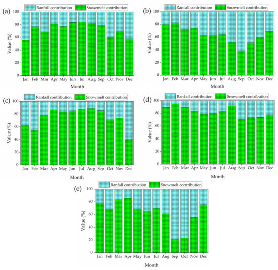
Figure 9.
Mean monthly rainfall and snowmelt contribution in the Upper Vakhsh River flow, using the SWAT model with (a) APHRODITE_V1101+CFSR, (b) APHRODITE_V1101+CRU TS3.1, (c) CFSR, (d) CRU TS3.1, and (e) observational datasets.

Figure 10.
Cumulative curves of the runoff input components for the Upper Vakhsh River, using the SWAT model with (a) APHRODITE_V1101+CFSR, (b) APHRODITE_V1101+CRU TS3.1, (c) CFSR, (d) CRU TS3.1, and (e) observational datasets.
Our study revealed that the gridded climate data from APHRODITE, CRU and CFSR can be used as alternative data, especially in areas with fewer climate stations, including the UVRB. These results represent the potential of the use of gridded datasets for hydrological modeling. If complete observational data are available for the reference period, it is more appropriate to use these data. In some cases, because of the provision of continuous data at spatial and temporal scales over a longer period, gridded datasets are preferred over observational datasets. The use of the most recently available gridded datasets in a consistent format and with improved technology has made them easier to use for hydrological modeling. Meanwhile, the combination of different gridded datasets can lead to improved hydrological modeling [82]. Similarly, we used the reference gridded datasets in combination, by combining their corresponding features with the daily measurement-based climate data to achieve evaluation and better model simulations. The snowmelt and rainfall contributions to annual river flow, according to the simulation results of the respective datasets, were different (Figure 9 and Figure 10). The differences in the contributions of the snowmelt and rainfall to annual river flow from the simulations of all combinations of datasets are due to the differences in the climate data. Such a difference may have occurred because the climate data came from different independent sources, with different approaches toward acquisition, processing data, and resolution. However, our results demonstrated that the gridded datasets performed well in capturing peak flows and base flows. The overall modeling results indicate that the SWAT model is potentially useful for studying hydrology and assessing the water yield of catchments.
Spring and summer runoff from the Vakhsh River Basin supplies several Central Asian countries, including Kyrgyzstan, Tajikistan, Uzbekistan and Turkmenistan, with water for domestic and agricultural needs, hydropower production and recreation [83]. Modeling the spring and summer snowmelt runoff is critical to understanding seasonal runoff variability. Water management and flood protection strategies in Central Asia are based on capturing and storing runoff for delivery in the fall months. Water managers track spring and summer runoff as a key factor when planning to meet Central Asia’s water supply needs [84]. It is also important to use spring and summer runoff data to predict the water supply and flooding in the basin.
5. Discussion
To the best of our knowledge, the simulation of the water balance component, particularly snowmelt runoff and its contribution to total runoff in the Vakhsh River Basin, has not been conducted previously. Similarly, an evaluation of the datasets’ ability to simulate the hydrological behavior of the UVRB from 1982 to 2006 has not previously been performed, especially not when using a combination of the APHRODITE_V1101+CFSR, AHPRODITE_V1101+CRU TS3.1, CFSR, and CRU TS3.1 datasets in a hydrological SWAT model. Water-balance elements in a catchment are influenced by climate and the physical characteristics of the basin, such as topography, land use, soil properties, glaciers, and human economic activities. For any analyses related to sustainable water resource management, understanding all the hydrological components is important. Snowmelt from the Vakhsh River is the main source of groundwater recharge and runoff in the dry seasons of many perennial rivers in Tajikistan, supplying fresh water for drinking, irrigation and hydropower generation. For this reason, it is very important to assess the contribution of snowmelt to the total runoff of UVRB for effective water resources management. Moreover, when modeling mountainous watershed hydrology, the most important determinant is the provision of accurate and alternative climate inputs in modeling. The lack of data has a large impact on modeling in mountainous regions. Ordinary climate stations are often scattered sparsely and cannot fully reflect the climatic conditions in the basin, especially in mountainous areas. In addition, the records of climate stations often do not cover the proposed modeling period or contain gaps. To address/mitigate this issue in UVRB CA, we examined the performance of gridded precipitation and temperature data combinations from various sources for simulating river flow, using the SWAT model.
In this study, the simulation of the observational-based datasets performed better than the gridded products in the UVRB for modeling river flow. Our results revealed that among the applied gridded datasets, the use of the CRU TS3.1 datasets for the overall scale (1982–2006) showed higher accuracy in river flow simulations, followed by the APHRODITE_V1101 and CRU TS3.1 combination, the APHRODITE_V1101 and CFSR combination, and the CFSR in the UVRB in Central Asia. Our results are consistent with those of Hajihosseini et al., who used the global CRU and SWAT models in the Upper Helmand Basin (UHB) in Afghanistan, which is a neighboring country to Tajikistan, to simulate the long-term hydrological conditions of the basin. Hajihosseini et al. used the CRU as an alternative data source, due to the lack of observational data at the UHB [30]. The results revealed the good performance of the SWAT model, using the CRU dataset for the UHB from 1969 to 1979, while NSE was 0.84 for the calibration period and 0.82 for the validation period [30]. As is similar to the results of our study, CRU datasets were used in the SWAT model to simulate river flows in the African continent over the period of 1968–1995, and the results showed a “good” performance (NSE > 0.6) [85]. However, our results for the CRU TS3.1 simulation contradicted the results of Malsy et al. [29], who examined the performance of hydrological modeling using four datasets, the Global Precipitation Climatology Centre (GPCC) Reanalysis product v6, APHRODITE, WATCH forcing data (WFD), and CRU, in a hydrological model (Water Global Assessment and Prognosis 3, WaterGAP 3) for the period from 1976 to 1999. According to Malsy et al., the GPCC and APHRODITE datasets with the WaterGAP 3 hydrological model showed better hydrological results than the CRU and WFD at the Tuul River Basin and Khovd River Basin in Mongolia in East Asia [29]. This contradiction may be associated with the use of a different hydrological model, a different selected period and a different study area location. It is not known if the same results could be generated in our study area with a different hydrological model. For instance, in the Hotan River Basin in southwestern Xinjiang in Central Asia, from 2004 to 2008, Luo et al. [31] assessed the performance of the SWAT and MIKE SHE hydrological models. The results showed that the SWAT model performs better (NSE = 0.77) than the MIKE SHE model (NSE = 0.66) for the same climate input. Besides hydrological modeling, the CRU dataset was evaluated for climatological studies in Central Asia by other researchers and their results showed that the CRU dataset is applicable and satisfactory for climatological studies in Central Asia [86,87].
Furthermore, our results indicated that a second alternative source for the hydrological simulation of the UVRB with the SWAT model could be the combination of precipitation with APHRODITE_V1101 and maximum/minimum temperature with CRU TS3.1, followed by the combination of APHRODITE_V1101 and CFSR, and CFSR. These results are in agreement with the findings of Tan et al. [34], who assessed the capabilities of the APHRODITE, CFSR and the “Precipitation Estimation from Remotely Sensed Information using Artificial Neural Networks” (PERSIANN) datasets to model river flow using the SWAT model for the Kelantan River Basin (KRB) and the Johor River Basin (JRB) in Malaysia in Southeast Asia, from 1985 to 1999. The combination of APHRODITE precipitation data and CFSR temperatures resulted in an accurate simulation of the river flow of the KRB and JRB. Tan et al. recommend the use of APHRODITE precipitation and CFSR temperature data when modeling the water resources of Malaysia [34]. Similarly, the APHRODITE dataset and the SWAT model were used for hydrological modeling from 1980 to 1989 in the Brahmaputra River Basin (BRB) and Yarlung Tsangpo River Basin (YTRB), which is the main international river flowing through China, Bhutan, India, and Bangladesh. The results showed the validity of APHRODITE estimates in driving the hydrological model in the YTRB and BRB [33]. Comparable results were reported by Xu et al. [35], who applied the SWAT model with APHRODITE and WFD in the Xiangjiang River Basin (XRB) in China to simulate river flow, particularly high flow and low flow. The APHRODITE simulation (NSE = 0.79, NSE = 0.82) performed better than the WFD dataset (NSE 0.69, NSE = 0.71), both during calibration (1991–2005) and validation (2001–2005) periods. WFD modeling leads to more errors in simulating flood events than APHRODITE [35]. The TRMM, NCEP, GPCP, CFSR and APHRODITE were used to assess the performance (NSE) of SWAT in the Wunna Basin in India [36]. APHRODITE dataset simulations performed much better (NSE = 0.68) than TRMM, NCEP, GPCP and CFSR, meaning that APHRODITE can be seen as an alternative source for hydrological modeling in the Wunna Basin [36]. Our results indicated the superiority of the combination of the APHRODITE_V1101 and CRU TS3.1 in the streamflow simulation in the UVRB from 1981 to 2006. However, these results are somewhat inconsistent with the findings of Eini et al. [88], who modeled hydrology systems and evaluated the performance of the SWAT model in the Maharlu Lake Basin in Iran by comparing CRU, NCEP CFSR, and APHRODITE, as well as reanalyzing Asfezari rainfall data using conventional data from 1983 to 2010. In this Iranian catchment, a simulation that was achieved through a combination of APHRODITE and CFSR showed superior performance (NSE = 0.91) compared to the other dataset combinations [88]. However, it should be noted that these results are region- and model-dependent. Many studies show that the accuracy of gridded data results varies by region [38,39]. Meanwhile, a hydrological model with a different concept and representation of the streamflow procedure may lead to different conclusions.
Our results demonstrated that for the overall scale (1982–2006), the CFSR simulated the hydrology of the UVRB with lower accuracy than APHRODITE_V1101+CFSR, APHRODITE_V1101+CRU TS3.1, and CRU TS3.1. Correspondingly, the simulation of river flow using a SWAT model based on the characteristics (NSE) of weather products, with reference to the CFSR, showed that despite the small number of observational climate stations in the basin, the modeling of observational datasets was more accurate for representing climate relationships in the basin than the CFSR. These results are very similar to those of Dile et al. [15] in the Gilgel Abay River and Gumera River in the Lake Tana Basin, and the upper part of the Upper Blue Nile Basin, where SWAT was also set up to assess the performance of CFSR datasets compared with conventional datasets for hydrological predictions from 1994 to 2008. Liu et al. [32] also used the SWAT model with climate data from the “China Meteorological Assimilation Driving Datasets” (CMADS V1.0) and CFSR in the Yellow River Source Basin, Qinghai–Tibet Plateau, from 2009 to 2013. Liu et al. found that the performance of the hydrological model for the monthly scale of CMADS (NSE = 0.78) was higher than that of the CFSR (NSE = 0.69) [32]. However, our results, as found in the UVRB, conflict with the findings of Tolere et al. [16], Fuka et al. [45], Cuceloglu and Ozturk [46], and Grusson et al. [89]. For instance, Tolere et al. [16] reported more successful SWAT streamflow simulation results using the CFSR than conventional datasets from 1990 to 1995 for the Keleta watershed in Ethiopia, where conventional data are scarce [16]. Fuka et al. [45] reported that the SWAT model presented better simulation results with CFSR datasets, compared to using traditional weather-gauging stations in the Catskill Mountains, NY, USA, and the Gumera Watershed in the Blue Nile River in Ethiopia, from 1996 to 2010. Similarly, Cuceloglu and Ozturk [46] evaluated CFSR using the SWAT model as a hydrological simulator in the Black Sea catchment from 2000 to 2012. The results showed that the CFSR gives quite reasonable agreement between simulated and observed river flow, compared to the observational dataset. Another study was conducted by Grusson et al. [89] in the Garonne River Watershed in France, employing CFSR and conventional datasets in hydrological simulations using the SWAT model from 2000 to 2010. The results revealed that the CFSR provided better hydrological simulations than conventional datasets [89]. Differences in climate and geographic conditions are the most likely explanation for such differences between the findings of Tolere et al. [16], Fuka et al. [45], Cuceloglu and Ozturk [46], Grusson et al. [89], and the results presented in this study.
The applicability of the SWAT model for the simulation of water balance components was assessed in the Heihe mountain river basin in northwest China, from 1961 to 1988 [22]. Water-balance components over the Narmada River Basin in India were assessed by Goswami et al. using the SWAT model and CFSR, from 1984 to 2013. The results suggested that the SWAT model was able to simulate the water-balance components at the basin and sub-basin scales [19]. Pathak et al. [90] applied the SWAT model in nine watersheds in India to validate the annual water yield obtained from diverse water-balance models. Moreover, Pathak et al. assessed the applicability of the Lumped Zhang model and InVEST model, together with the SWAT model, to compute water yield in scenarios before and after climate change for 1980, 1990, 2001, and 2015 [90]. Gupta et al. [18] estimated the water-balance components in the Sabarmati River Basin (SRB) in India using the SWAT model, from 1999 to 2005. Gupta et al. noted that SWAT is a powerful tool that very effectively evaluated hydrological components in the study of the water balance and river flow of the SRB [18]. In Nepal, Thapa et al. used the HBV and BTOPMC models, along with the SWAT model, to assess the components of water balance from 2001 to 2010. The results of the three models were similar [91]. A predictive study using three models also offered a reasonable range for runoff and evapotranspiration estimates [91]. Water balance and water yield were predicted by the SWAT model in a basin in the north-central part of Nigeria, from 1985 to 2010 [17]. Adeogun et al. noted that the SWAT model can be a promising tool for predicting water balance, in terms of sustainable water management in Nigeria [17]. The SWAT model was applied by Leta et al. to model water balance components in the Heeia watershed in Hawai’i, an island in the Pacific Ocean, from 2006 to 2013 [92]. This study demonstrated the applicability of SWAT to small island watersheds with large topographic, precipitation, and land-use gradients. Our seasonal and annual precipitation results in the UVRB in Central Asia, using the APHRODITE_V1101 and CRU TS3.1, demonstrated much closer results to the observational dataset. These findings are in agreement with the results of a study by Shen et al. in the Kaidu Basin in Central Asia. Shen et al. [37] used gridded products, including CFSR, APHRODITE, CRU, TRMM, ERA-Interim and MERRA-2, with the J2000 model to analyze the spatiotemporal patterns of water balance and the distribution of runoff components in the glacierized Kaidu Basin in Central Asia. The results showed that APHRODITE and CRU represented annual and seasonal precipitation dynamics that were similar to the observational dataset at most climate points [37]. Similarly, a water balance study with the application of the SWAT model and observational datasets was conducted in the Indian Ken River Basin in South Asia, from 1986 to 2005 [20]. Himanshu et al. concluded that the SWAT model can accurately simulate the hydrology of the Ken River Basin in India. The water balance study of the basin showed that evapotranspiration is more predominant, accounting for about 44.6% of the average annual precipitation [20].
In this study, considering the more accurate performance of the CRU TS3.1 and observational datasets than other studied datasets, the simulations of the CRU TS3.1 and observational datasets showed that the actual evapotranspiration in July is almost equal to the July catchment precipitation values. These results are in accordance with those of Pritchard [23], who used a combination of CFSR temperature and APHRODITE precipitation datasets in the SWAT model to simulate water-balance components, especially the actual evapotranspiration in five Asian river basins, including the Aral, Indus, Ganges, Brahmaputra, Tarim, and the lakes of Issyk-Kul and Balkhash. For the Aral Sea Basin in Central Asia, Pritchard reported that summer evaporation is approximately equal to summer precipitation [23]. In this study, less actual evapotranspiration occurs in December, January, and February for all datasets studied, including CFSR. However, this result contradicts the findings of Goswami et al. [19], who found that the simulations of actual evapotranspiration showed minimal values in May, using CFSR and the SWAT model, in the Narmada River Basin of India in South Asia between 1984 and 2013. The results of our simulation showed that the average annual actual evapotranspiration is about 2.9% (CFSR), 9.93% (APHRODITE_V1101+CFSR), 21.1% (CRU TS3.1), 25.52% (APHRODITE_V1101+CRU TS3.1), and 27.28% (observational datasets) of the average annual precipitation in the UVRB from 1982 to 2006. The same methodology was applied by Budhathoki et al. [93] in the West Seti River Basin (WSRB) in South Asia, to simulate the mean annual water balance components, including precipitation and evapotranspiration, using the SWAT model and a combination of conventional weather data and APHRODITE, for the period of 1986–2005. The mean annual total evapotranspiration matched about 36% of the mean annual precipitation in the WSRB [93]. In another study, Nasiri et al. [21] applied the SWAT model to the Samalqan Basin in Iran in Western Asia, from 2004 to 2014, to compute actual evapotranspiration using observational weather data. Actual evapotranspiration contributed to the largest water loss from the basin, at approximately 86%. Nasiri et al. pointed out that the high evapotranspiration rate that was simulated may be related to the vegetation types in the region [21].
Our results indicated that the simulation of the CFSR provided lower actual evapotranspiration values than traditional weather data for the UVRB from 1981 to 2006. Similar results were obtained by Dile et al. [16] in the Gumera, Rib and Megech River Basins in Ethiopia in the Horn of Africa, where independent observation datasets and CFSR were used in the SWAT model in 1990–1995 [16]. However, Dile et al. stated that the results in the Melka Kuntur Basin showed higher values for the water-balance components; this may be due to the relatively high total precipitation in the CFSR dataset in the Melka Kuntur Basin [16]. In general, in our study, CFSR also simulated higher total annual precipitation in the UVRB in Central Asia, compared to other reference datasets. We found the largest deviation between the monthly mean actual evapotranspiration CFSR and the observational datasets, compared to other applied datasets in the UVRB. However, from previous studies, we have observed that in some regions, CFSR, when calculating actual evapotranspiration, produced values very similar to conventional weather data. For instance, the CFSR and observational datasets, with the SWAT model, were applied to different watersheds in the Blue Nile Basin in the northwestern Ethiopian Plateau from 1994 to 2008, to estimate actual evapotranspiration [15]. For the Megech sub-basins in Ethiopia, the results showed that the deviation between the monthly mean actual evapotranspiration levels, obtained from CFSR simulations, and observational datasets was less than mm in all months besides August and September, when it reached 12 mm and 19 mm, respectively. Dile et al. noted that CFSR weather data can be a valuable option for hydrological prediction where conventional data are not available, such as in remote parts of the Upper Blue Nile Basin [15].
Based on the SWAT model application, our results for the simulations of five different climate data combinations, including APHRODITE_V1101+CFSR, APHRODITE_V1101+CRU TS3.1, CFSR, CRU TS3.1, and observational data showed that approximately 81.06%, 63.12%, 82.79%, 81.66%, and 67.67% of annual runoff was contributed by snowmelt runoff from 1982 to 2006 in the UVRB. The largest contribution of snowmelt runoff to the total runoff appears during the spring and summer periods. The monthly APHRODITE_V1101+CFSR simulations showed that from May to August, the snowmelt runoff contribution to river flow was about 68.10% (March), 80.75% (April), 76.97% (May), 83.41% (June), 84.15% (July), and 82.66% (August); for the APHRODITE_V1101+CRU TS3.1 simulations, it was about 72.49%, 73.63%, 62.24%, 63.36%, 63.86%, and 51.29%; for the CFSR simulations, it was about 77.57%, 86.47%, 82.90%, 84.95%, 86.98%, and 88.72%; for the CRU TS3.1 simulations, it was about 89.05%, 83.17%, 78.33%, 79.93%, 83.41%, and 91.75%; and, for the observational simulations, it was about 83.13%, 85.60%, 67.58%, 64.41%, 69.43%, and 60.49%. Many studies have shown that the application of the SWAT model is quite useful in snowmelt simulations [1,2,24,25]. As far as we are aware, in this study, the use of the SWAT model with various combinations of the respective climate datasets was conducted for the first time as a way to simulate snowmelt runoff contribution to river flow in this mountainous basin.
By using observational climate data in the SWAT model, Duan et al. simulated the snowmelt contribution to total runoff in the Tizinafu River Basin (TRB) in Xinjiang in Central Asia, from 2013 to 2014 [25]. Duan et al. found that about 44.7% of the total runoff comes from snowmelt runoff in the TRB [25]. Siderius et al. [24] calculated the contribution of snowmelt to river runoff using APHRODITE data with the SWAT model, from 1971 to 2000, in the Ganges River in northern India in the Himalayan arc in South Asia. The SWAT results showed that approximately 1% and 5% can be considered to be indicative of the actual total annual contribution of snowmelt to total runoff. The contribution of seasonal snowmelt to total runoff during the dry season before the summer monsoon (MAM) is estimated to range from 12% to 38% [24]. A similar approach was applied by Chiphang et al. [1], who used the SWAT model in the mountainous Mago River Basin, located in the Eastern Himalayan region of India, from 2006 to 2009 to compute the contribution of snowmelt to streamflow changes in the basin. Their results showed that the contribution of snowmelt runoff to the annual streamflow of the basin was about 8% [1]. Another study was performed by Dhami et al. using the snowmelt runoff model (SRM) and SWAT model with conventional weather data, to compute the water balance components of the Karnali River Basin in Nepal in South Asia and to simulate the contribution of snowmelt to river runoff, from 1993 to 2005 [2]. Dhami et al. reported that, from the comparison of the results obtained from the SWAT model and the SRM model, it is recommended that the results obtained from the SWAT model are used due to its better performance in terms of predicting reality than the SRM model [2]. The results of the SWAT model indicated that in the Karnali River Basin, about 35% of the total runoff is contributed by snowmelt runoff [2]. An accurate representation of the snowmelt process could improve the prediction of streamflow in mountainous catchments [89,94]. The UVRB has good seasonal snow cover at high altitudes. Snowmelt is usually an important source of river flow at high altitudes. In this study, SWAT appropriately demonstrates both the beginning of snowmelt and the peak of spring snowmelt.
The perennial river basin system, when combined with steep slopes, provides enormous hydropower potential, the exploitation of which requires a deep understanding of the hydrological system of the catchment. The capacity of hydropower is determined by the flow rate of the river, so a change in flow will directly lead to changes in hydropower potential [95]. Determining the effect of snowmelt on streamflow in the catchment allows an assessment of the hydrological processes within a river basin in a mountainous region. Snowmelt tends to create regular seasonal patterns of river flow during warmer temperatures, with the melting of snowpacks accumulated over the winter. The impact of melting snow on potential flooding, mainly in the spring, is of concern to many inhabitants across the globe. The performance of the SWAT model presents evidence that it can be applied efficiently in the transboundary Vakhsh River Basin in Central Asia for water resources assessment and management. Semi-distributed hydrological models can be used as an essential feature of the water resources monitoring approach and can play a crucial part in the management of transboundary water resources [96]. Furthermore, well-calibrated models are an important tool for a variety of water management applications, such as for assessing the availability and balance of water resources, modeling water quality and sediment transport, etc.
Uncertainties and Limitations
The SWAT model has been applied in several hydrological modeling studies in various catchments around the world [14,25,97]. There may be a few areas of uncertainty in modeling snow and glacier melt, such as orographic impacts and hydrological model parameterization, as well as heterogeneity in forest cover, slope, and features, which are evident issues in snow and glacier hydrology. All of these aspects are not well represented by a simple temperature index of snowmelt and glacier melt simulation. However, the evaluation of snowmelt based on a temperature index appears to be good enough to compute the physics of snowmelt processes entirely. Snowmelt hydrology is specifically considered as an essential variable in local catchments. Due to the degree-day approach with elevation bands in the SWAT snowmelt module, it is hard to avoid the uncertainties inherent in the model structure, parameters and input data. On the other hand, the absence of an ice-melt module would also cause potential uncertainties. Calibration solely by discharge records might produce good results, as well as potential uncertainties [8]. Parameter uncertainty occurs when certain physical processes in a hydrological or climatic system cannot be explicitly resolved. As a replacement, they must be included via parameterization, which contains some uncertain variables. The UVRB is situated in a mountainous area, within which a wide range of regions subject to permafrost and seasonal cold is spread. The freezing/thawing processes of the soil also affect the accuracy of the simulation [98]. Furthermore, measurement-based flow data that have been used in a comparison with a simulated flow may be exposed to human or tool errors in river-level observations, or inaccuracies in estimated curves, all of which are designed for natural river stretches that are subject to erosion and deposition [99]. The uncertainty of the data source stems from the use of the CRU, which is generated by interpolating data from weather stations in the region. Therefore, the entered climatic data are approximate [100]. The APHRODITE dataset, which includes multiple climate stations, provides high-resolution, gridded, long-term daily precipitation estimates, as commonly used in South Asia. In the UVRB, most of the climate stations are located in valleys and are not in mountains with a large amount of precipitation. The combination of all of these factors can increase the uncertainty of the APHRODITE estimates. Precipitation data from CFSR showed more heterogeneity than the temperature data. The gridded dataset was obtained directly; thus, its applicability in the study region must be assessed prior to its use. The precipitation error characteristics of datasets vary due to climatic regions, elevations, surface conditions, seasons and storm patterns [101]. Similarly, these datasets are inevitably prone to inaccuracies caused by sampling uncertainties, indirect measurements, and exploration algorithms [102]. In future investigations, it might be possible to analyze the effects of bias correction on multiple gridded climate data estimates in SWAT hydrological element simulations.
6. Conclusions
We used the SWAT–CUP Sequential Uncertainty Fitting (SUFI-2) program to assess the water balance components of the basin. APHRODITE_V1101, CFSR, and CRU TS3.1 gridded datasets were tested both independently and in combination with observational datasets for hydrological simulation. The SWAT hydrological model was used to examine the datasets in Central Asia’s Vakhsh River Basin. We also tested the SWAT model’s applicability to the UVRB hydrology. The authors came to the following conclusions:
- (a)
- The results of the study indicated that the applied gridded datasets, such as CRU TS3.1, AHPRODITE_V1101, and CFSR, can be used as alternative climate data in an assessment of the hydrology in the UVRB.
- (b)
- We observed that the CFSR datasets performed worse than APHRODITE_V1101+CFSR, APHRODITE_V1101+CRU TS3.1, and observational datasets.
- (c)
- Aquifer percolation fraction (RCHRG_DP), baseflow alpha-factor (ALPHA_BF), moist bulk density (SOL_BD), SCS runoff curve number for moisture condition-II (CN2), and effective hydraulic conductivity in main channel alluvium (CH_K2) were determined to be the most sensitive factors for streamflow simulation using the SWAT model in the UVRB.
- (d)
- APHRODITE_V1101+CFSR showed “good” [71] results in simulating the monthly observed streamflow (with NSE = 0.70 and 0.72 for calibration and for overall period, respectively, and PBIAS = 14.8% and 15% for calibration and for overall period, respectively). The APHRODITE_V1101+CRU TS3.1 gave “good” results for calibration and overall periods (NSE = 0.74 and 0.74, respectively), with “satisfactory” [71] (PBIAS = −17.7%) and “good” (PBIAS = −10.80%) underestimation of streamflow. This combination showed “very good” [71] results (NSE = 0.78) for the validation period with a “very good” overestimation of streamflow (PBIAS of 1.30%). The CFSR datasets presented “good” results (NSE = 0.68) with a “very good” (PBIAS of 2%) overestimation of streamflow and, for the validation period, CFSR provided “very good” results (NSE = 0.83) with a “very good” overestimation of streamflow (PBIAS of 9.58%). The CRU TS3.1 datasets gave “very good” results for calibration, validation and overall scales (NSE = 0.91, 0.88 and 0.91, and PBIAS = 0.32%, 6.09%, and 0.29%, respectively). The observational datasets for calibration, validation and overall provided “very good” results (NSE = 0.90, 0.93 and 0.91 and PBIAS = 0.69%, 5.51%, and 5.21%, respectively). The better performance corresponds to observational datasets with higher NSE values, followed by the CRU TS3.1 datasets.
- (e)
- The coefficient of determination (R2) showed an acceptable (>0.6) [103] correlation between the observed and simulated monthly streamflow during calibration, validation, and overall scales (R2 ranges from 0.74 to 0.94) for all five datasets.
- (f)
- For APHRODITE_V1101+CFSR, APHRODITE_V1101+CRU TS3.1, CFSR, CRU TS3.1, and observational datasets, the SWAT model simulated mean annual precipitation of the UVRB as 1875.9 mm, 1236.9 mm, 2479 mm, 1215.9 mm, and 1098.5 mm, respectively, with 93.82% (1760.11 mm), 70.41% (870.85 mm), 96% (2379.86 mm), 86.52% (1051.98 mm), and 76.16% (836.65 mm) as snowfall, out of which 29.70% (522.72 mm), 72.19% (628.63 mm), 25.88% (615.80 mm), 68.51% (720.67 mm), and 68.87% (576.19 mm), respectively, melts and facilitates snowmelt runoff in the basin.
- (g)
- The UVR basin evapotranspiration is 9.93% (APHRODITE_V1101+CFSR), 25.52% (APHRODITE_V1101+CRU TS3.1), 2.9% (CFSR), 21.08% (CRU TS3.1), and 27.28% (observational datasets) (186.3 mm, 315.7 mm, 72.1 mm, 256.4 mm, and 299.7 mm out of 1875.9 mm, 1236.9 mm, 2479 mm, 1215.9 mm, and 1098.5 mm, respectively). Overall, less evapotranspiration occurs in December, January, and February.
- (h)
- From 1982 to 2006, the simulation of five different weather products (APHRODITE_V1101+CFSR, APHRODITE_V1101+CRU TS3.1, CFSR, CRU TS3.1) and observational datasets in the UVR basin showed that snowmelt runoff contributes approximately 81.06%, 63.12%, 82.79%, 81.66%, and 67.67%, respectively, of annual runoff. Snowmelt runoff contributes the most to overall runoff in spring and summer.
- (i)
- The annual flow contribution of rain was estimated at 18.94%, 36.88%, 17.21%, 18.34%, and 32.33% using APHRODITE_V1101+CFSR, APHRODITE_V1101+CRU TS3.1, CFSR, CRU TS3.1, and observational datasets.
The SWAT hydrological simulation of observational datasets outperformed gridded products in the mountainous UVRB. The SWAT model-simulated streamflow variations better than CFSR gridded datasets using CRU TS3.1 and APHRODITE_V1101. Gridded meteorological datasets like CRU TS3.1, APHRODITE_V1101, and CFSR can also be used for hydrologic modeling, especially if observational data is scarce. The SWAT model captured the monthly observed flow patterns and trends well. The model produced reliable monthly streamflow estimates, as evidenced by NSE, R2, and PBIAS values that were superior for calibration, validation, and overall scales. The high NSE, R2, and PBIAS values for monthly streamflow during the calibration, validation and overall periods indicate the model’s predictive ability. For water management challenges in the basin, the SWAT model offered a baseline understanding of hydrological dynamics. The current study demonstrates that the SWAT model could be a helpful tool for predicting water balance components to assist basin-level policies and decisions.
Author Contributions
All authors were involved in the intellectual elements of this paper. X.C., A.G., and T.L. designed the research. A.G. conducted the research and wrote the manuscript. N.G. and M.G. helped in the data arrangement and data analysis. J.P. and Z.L. helped in the validation. T.L. and Z.K. helped revise the manuscript and also provided many suggestions. All authors have read and agreed to the published version of the manuscript.
Funding
This study was financially supported by the Strategic Priority Research Program of the Chinese Academy of Sciences, the Pan-Third Pole Environment Study for a Green Silk Road (Grant No. XDA20060303), the project of Research Center for Ecology and Environment of Central Asia (Grant No. Y934031),the International Cooperation Project of National Natural Science Foundation of China (Grant No. 41761144079),the CAS PIFI fellowship (Grant No. 2021PC0002), the Xinjiang Tianchi Hundred Talents Program (Grant No. Y848041), the CAS Inter-displinary Innovation Team (Grant No. JCTD-2019-20), and the Regional Collaborative Innovation Project of Xinjiang Uygur Autonomous Regions (Grant No. 2020E01010).
Institutional Review Board Statement
Not applicable.
Informed Consent Statement
Not applicable.
Data Availability Statement
The data of this research in the Upper Vakhsh River Basin was offered by Ministry of Energy and Water Resources of the Republic of Tajikistan and the Agency of Hydrometeorology of the Committee for Environmental Protection under the Government of the Republic of Tajikistan.
Acknowledgments
The authors are thankful to the Ministry of Energy and Water Resources of the Republic of Tajikistan and the Agency of Hydrometeorology of the Committee for Environmental Protection under the Government of the Republic of Tajikistan for providing the data for this research.
Conflicts of Interest
The authors declare no conflict of interest.
References
- Chiphang, N.; Bandyopadhyay, A.; Bhadra, A. Assessing the Effects of Snowmelt Dynamics on Streamflow and Water Balance Components in an Eastern Himalayan River Basin Using SWAT Model. Environ. Model. Assess. 2020, 25, 861–883. [Google Scholar] [CrossRef]
- Dhami, B.; Himanshu, S.K.; Pandey, A.; Gautam, A.K. Evaluation of the SWAT model for water balance study of a mountainous snowfed river basin of Nepal. Environ. Earth Sci. 2018, 77, 21. [Google Scholar] [CrossRef]
- Schuol, J.; Abbaspour, K. Using monthly weather statistics to generate daily data in a SWAT model application to West Africa. Ecol. Model. 2007, 201, 301–311. [Google Scholar] [CrossRef]
- Liu, Z.J.; Weller, D.E.; Jordan, T.E.; Correll, D.L.; Boomer, K.B. Integrated Modular Modeling of Water and Nutrients From Point and Nonpoint Sources in the Patuxent River Watershed 1. JAWRA J. Am. Water Resour. Assoc. 2008, 44, 700–723. [Google Scholar] [CrossRef]
- Abbott, M.; Bathurst, J.; Cunge, J.; O’connell, P.; Rasmussen, J. An introduction to the European Hydrological System—Systeme Hydrologique Europeen,“SHE”, 2: Structure of a physically-based, distributed modelling system. J. Hydrol. 1986, 87, 61–77. [Google Scholar] [CrossRef]
- Arnold, J.G.; Srinivasan, R.; Muttiah, R.S.; Williams, J.R. Large area hydrologic modeling and assessment part I: Model development 1. JAWRA J. Am. Water Resour. Assoc. 1998, 34, 73–89. [Google Scholar] [CrossRef]
- Holtan, H.N.; Lopez, N.C. USDAHL-70 Model of Watershed Hydrology; US Department of Agriculture, U.S. Government Printing Office: Washington, DC, USA, 1971. [Google Scholar]
- Fontaine, T.; Cruickshank, T.; Arnold, J.; Hotchkiss, R. Development of a snowfall–snowmelt routine for mountainous terrain for the soil water assessment tool (SWAT). J. Hydrol. 2002, 262, 209–223. [Google Scholar] [CrossRef]
- Abbaspour, K. User Manual for SWAT-CUP, SWAT Calibration and Uncertainty Analysis Programs; Swiss Federal Institute of Aquatic Science and Technology: Eawag, Switzerland, 2007. [Google Scholar]
- Debele, B.; Srinivasan, R.; Gosain, A. Comparison of process-based and temperature-index snowmelt modeling in SWAT. Water Resour. Manag. 2010, 24, 1065–1088. [Google Scholar] [CrossRef]
- Pradhanang, S.M.; Anandhi, A.; Mukundan, R.; Zion, M.S.; Pierson, D.C.; Schneiderman, E.M.; Matonse, A.; Frei, A. Application of SWAT model to assess snowpack development and streamflow in the Cannonsville watershed, New York, USA. Hydrol. Process. 2011, 25, 3268–3277. [Google Scholar] [CrossRef]
- Troin, M.; Caya, D. Evaluating the SWAT’s snow hydrology over a Northern Quebec watershed. Hydrol. Process. 2014, 28, 1858–1873. [Google Scholar] [CrossRef]
- Zhang, L.; Jin, X.; He, C.; Zhang, B.; Zhang, X.; Li, J.; Zhao, C.; Tian, J.; DeMarchi, C. Comparison of SWAT and DLBRM for hydrological modeling of a mountainous watershed in arid northwest China. J. Hydrol. Eng. 2016, 21, 04016007. [Google Scholar] [CrossRef]
- Omani, N.; Srinivasan, R.; Karthikeyan, R.; Reddy, V.; Smith, P.K. Impacts of climate change on the glacier melt runoff from five river basins. Trans. ASABE 2016, 59, 829–848. [Google Scholar]
- Dile, Y.T.; Srinivasan, R. Evaluation of CFSR climate data for hydrologic prediction in data-scarce watersheds: An application in the Blue Nile River Basin. JAWRA J. Am. Water Resour. Assoc. 2014, 50, 1226–1241. [Google Scholar] [CrossRef]
- Tolera, M.B.; Chung, I.-M.; Chang, S.W. Evaluation of the climate forecast system reanalysis weather data for watershed modeling in Upper Awash basin, Ethiopia. Water 2018, 10, 725. [Google Scholar] [CrossRef] [Green Version]
- Adeogun, A.G.; Sule, B.F.; Salami, A.W.; Daramola, M.O. Validation of SWAT model for prediction of water yield and water balance: Case study of upstream catchment of Jebba dam in Nigeria. Int. J. Math. Comput. Phys. Comput. Eng. 2014, 8, 264–270. [Google Scholar]
- Gupta, A.; Himanshu, S.K.; Gupta, S.; Singh, R. Evaluation of the SWAT Model for Analysing the Water Balance Components for the Upper Sabarmati Basin. In Advances in Water Resources Engineering and Management; Springer: Singapore, 2020; pp. 141–151. [Google Scholar]
- Goswami, S.B.; Kar, S.C. Simulation of water cycle components in the Narmada River basin by forcing SWAT model with CFSR data. Meteorol. Hydrol. Water Manag. Res. Oper. Appl. 2018, 13–25, 6. [Google Scholar] [CrossRef]
- Himanshu, S.K.; Pandey, A.; Shrestha, P. Application of SWAT in an Indian river basin for modeling runoff, sediment and water balance. Environ. Earth Sci. 2017, 76, 3. [Google Scholar] [CrossRef]
- Nasiri, S.; Ansari, H.; Ziaei, A.N. Simulation of water balance equation components using SWAT model in Samalqan Watershed (Iran). Arab. J. Geosci. 2020, 13, 421. [Google Scholar] [CrossRef]
- Yin, Z.; Feng, Q.; Zou, S.; Yang, L. Assessing variation in water balance components in mountainous inland river basin experiencing climate change. Water 2016, 8, 472. [Google Scholar] [CrossRef] [Green Version]
- Pritchard, H.D. Asia’s glaciers are a regionally important buffer against drought. Nature 2017, 545, 169–174. [Google Scholar] [CrossRef]
- Siderius, C.; Biemans, H.; Wiltshire, A.; Rao, S.; Franssen, W.; Kumar, P.; Gosain, A.; Van Vliet, M.; Collins, D. Snowmelt contributions to discharge of the Ganges. Sci. Total Environ. 2013, 468, S93–S101. [Google Scholar] [CrossRef] [PubMed]
- Duan, Y.; Liu, T.; Meng, F.; Luo, M.; Frankl, A.; De Maeyer, P.; Bao, A.; Kurban, A.; Feng, X. Inclusion of modified snow melting and flood processes in the swat model. Water 2018, 10, 1715. [Google Scholar] [CrossRef] [Green Version]
- Mohammed, I.N.; Bolten, J.D.; Srinivasan, R.; Lakshmi, V. Satellite observations and modeling to understand the Lower Mekong River Basin streamflow variability. J. Hydrol. 2018, 564, 559–573. [Google Scholar] [CrossRef] [PubMed]
- Tan, M.L.; Samat, N.; Chan, N.W.; Roy, R. Hydro-meteorological assessment of three GPM satellite precipitation products in the Kelantan River Basin, Malaysia. Remote Sens. 2018, 10, 1011. [Google Scholar] [CrossRef] [Green Version]
- Li, D.; Christakos, G.; Ding, X.; Wu, J. Adequacy of TRMM satellite rainfall data in driving the SWAT modeling of Tiaoxi catchment (Taihu lake basin, China). J. Hydrol. 2018, 556, 1139–1152. [Google Scholar] [CrossRef]
- Malsy, M.; aus der Beek, T.; Flörke, M. Evaluation of large-scale precipitation data sets for water resources modelling in Central Asia. Environ. Earth Sci. 2015, 73, 787–799. [Google Scholar] [CrossRef]
- Hajihosseini, H.; Hajihosseini, M.; Morid, S.; Delavar, M.; Booij, M.J. Hydrological assessment of the 1973 treaty on the transboundary Helmand River, using the SWAT model and a global climate database. Water Resour. Manag. 2016, 30, 4681–4694. [Google Scholar] [CrossRef]
- Luo, M.; Meng, F.; Liu, T.; Duan, Y.; Frankl, A.; Kurban, A.; De Maeyer, P. Multi–model ensemble approaches to assessment of effects of local Climate Change on water resources of the Hotan River Basin in Xinjiang, China. Water 2017, 9, 584. [Google Scholar] [CrossRef]
- Liu, J.; Shanguan, D.; Liu, S.; Ding, Y. Evaluation and hydrological simulation of CMADS and CFSR reanalysis datasets in the Qinghai-Tibet Plateau. Water 2018, 10, 513. [Google Scholar] [CrossRef] [Green Version]
- Luo, X.; Fan, X.; Ji, X.; Li, Y. Evaluation of corrected APHRODITE estimates for hydrological simulation in the Yarlung Tsangpo–Brahmaputra River Basin. Int. J. Climatol. 2019, 40, 4158–4170. [Google Scholar] [CrossRef]
- Tan, M.L.; Gassman, P.W.; Cracknell, A.P. Assessment of three long-term gridded climate products for hydro-climatic simulations in tropical river basins. Water 2017, 9, 229. [Google Scholar] [CrossRef] [Green Version]
- Xu, H.; Xu, C.-Y.; Chen, S.; Chen, H. Similarity and difference of global reanalysis datasets (WFD and APHRODITE) in driving lumped and distributed hydrological models in a humid region of China. J. Hydrol. 2016, 542, 343–356. [Google Scholar] [CrossRef]
- Singh, L.; Saravanan, S. Evaluation of various spatial rainfall datasets for streamflow simulation using SWAT model of Wunna basin, India. Int. J. River Basin Manag. 2020, 20, 1–25. [Google Scholar] [CrossRef]
- Shen, Y.J.; Shen, Y.; Fink, M.; Kralisch, S.; Brenning, A. Unraveling the Hydrology of the glacierized Kaidu Basin by integrating multisource data in the Tianshan Mountains, Northwestern China. Water Resour. Res. 2018, 54, 557–580. [Google Scholar] [CrossRef]
- Yatagai, A.; Krishnamurti, T.; Kumar, V.; Mishra, A.; Simon, A. Use of APHRODITE rain gauge–based precipitation and TRMM 3B43 products for improving Asian monsoon seasonal precipitation forecasts by the superensemble method. J. Clim. 2014, 27, 1062–1069. [Google Scholar] [CrossRef]
- Li, L.; Ngongondo, C.S.; Xu, C.-Y.; Gong, L. Comparison of the global TRMM and WFD precipitation datasets in driving a large-scale hydrological model in southern Africa. Hydrol. Res. 2013, 44, 770–788. [Google Scholar] [CrossRef]
- Gulakhmadov, A.; Chen, X.; Gulahmadov, N.; Liu, T.; Davlyatov, R.; Sharofiddinov, S.; Gulakhmadov, M. Long-Term Hydro–Climatic Trends in the Mountainous Kofarnihon River Basin in Central Asia. Water 2020, 12, 2140. [Google Scholar] [CrossRef]
- Vaghefi, S.A.; Abbaspour, N.; Kamali, B.; Abbaspour, K.C. A toolkit for climate change analysis and pattern recognition for extreme weather conditions–Case study: California-Baja California Peninsula. Environ. Model. Softw. 2017, 96, 181–198. [Google Scholar] [CrossRef]
- Touseef, M.; Chen, L.; Yang, K.; Chen, Y. Long-Term Rainfall Trends and Future Projections over Xijiang River Basin, China. Adv. Meteorol. 2020, 2020, 6852148. [Google Scholar] [CrossRef] [Green Version]
- Yatagai, A.; Kamiguchi, K.; Arakawa, O.; Hamada, A.; Yasutomi, N.; Kitoh, A. APHRODITE: Constructing a long-term daily gridded precipitation dataset for Asia based on a dense network of rain gauges. Bull. Am. Meteorol. Soc. 2012, 93, 1401–1415. [Google Scholar] [CrossRef]
- Palazzi, E.; Von Hardenberg, J.; Provenzale, A. Precipitation in the Hindu-Kush Karakoram Himalaya: Observations and future scenarios. J. Geophys. Res. Atmos. 2013, 118, 85–100. [Google Scholar] [CrossRef]
- Fuka, D.R.; Walter, M.T.; MacAlister, C.; Degaetano, A.T.; Steenhuis, T.S.; Easton, Z.M. Using the Climate Forecast System Reanalysis as weather input data for watershed models. Hydrol. Process. 2014, 28, 5613–5623. [Google Scholar] [CrossRef]
- Cuceloglu, G.; Ozturk, I. Assessing the Impact of CFSR and Local Climate Datasets on Hydrological Modeling Performance in the Mountainous Black Sea Catchment. Water 2019, 11, 2277. [Google Scholar] [CrossRef] [Green Version]
- Worqlul, A.W.; Yen, H.; Collick, A.S.; Tilahun, S.A.; Langan, S.; Steenhuis, T.S. Evaluation of CFSR, TMPA 3B42 and ground-based rainfall data as input for hydrological models, in data-scarce regions: The upper Blue Nile Basin, Ethiopia. Catena 2017, 152, 242–251. [Google Scholar] [CrossRef]
- Jarvis, A.; Reuter, H.I.; Nelson, A.; Guevara, E. Hole-Filled SRTM for the Globe Version 4. 2008. Available online: http://srtm.csi.cgiar.org (accessed on 16 July 2020).
- Food and Agriculture Organization; International Institute for Applied Systems Analysis; International Soil Reference and Information Centre. JRC: Harmonized World Soil Database (Version 1.2); FAO: Rome, Italy; IIASA: Laxenburg, Austria, 2012. [Google Scholar]
- Arino, O.; Ramos Perez, J.J.; Kalogirou, V.; Bontemps, S.; Defourny, P.; Van Bogaert, E. Global Land CoverMap for 2009 (GlobCover 2009); European Space Agency: Paris, France; University College London: London, UK, 2012. [Google Scholar]
- Yacoub, C.; Foguet, A.P. Slope effects on SWAT modeling in a mountainous basin. J. Hydrol. Eng. 2013, 18, 1663–1673. [Google Scholar] [CrossRef] [Green Version]
- Neitsch, S.L.; Arnold, J.G.; Kiniry, J.R.; Williams, J.R. Soil and Water Assessment Tool Theoretical Documentation Version 2009; Texas Water Resources Institute: Temple, TX, USA, 2011. [Google Scholar]
- Gassman, P.W.; Reyes, M.R.; Green, C.H.; Arnold, J.G. The soil and water assessment tool: Historical development, applications, and future research directions. Trans. ASABE 2007, 50, 1211–1250. [Google Scholar] [CrossRef] [Green Version]
- Cronshey, R. Urban Hydrology for Small Watersheds; US Department of Agriculture, Soil Conservation Service, Engineering Division: Washington, DC, USA, 1986. [Google Scholar]
- Hydrology, S. National Engineering Handbook; US Soil Conservation Service: Washington, DC, USA, 1972. [Google Scholar]
- Hock, R. Temperature index melt modelling in mountain areas. J. Hydrol. 2003, 282, 104–115. [Google Scholar] [CrossRef]
- Rahman, K.; Maringanti, C.; Beniston, M.; Widmer, F.; Abbaspour, K.; Lehmann, A. Streamflow modeling in a highly managed mountainous glacier watershed using SWAT: The Upper Rhone River watershed case in Switzerland. Water Resour. Manag. 2013, 27, 323–339. [Google Scholar] [CrossRef] [Green Version]
- Ruan, H.; Zou, S.; Yang, D.; Wang, Y.; Yin, Z.; Lu, Z.; Li, F.; Xu, B. Runoff simulation by SWAT model using high-resolution gridded precipitation in the upper Heihe River Basin, Northeastern Tibetan Plateau. Water 2017, 9, 866. [Google Scholar] [CrossRef] [Green Version]
- Omani, N.; Srinivasan, R.; Karthikeyan, R.; Smith, P.K. Hydrological modeling of highly glacierized basins (Andes, Alps, and Central Asia). Water 2017, 9, 111. [Google Scholar] [CrossRef] [Green Version]
- Garee, K.; Chen, X.; Bao, A.; Wang, Y.; Meng, F. Hydrological modeling of the upper indus basin: A case study from a high-altitude glacierized catchment Hunza. Water 2017, 9, 17. [Google Scholar] [CrossRef] [Green Version]
- Gulakhmadov, A.; Chen, X.; Gulahmadov, N.; Liu, T.; Anjum, M.N.; Rizwan, M. Simulation of the Potential Impacts of Projected Climate Change on Streamflow in the Vakhsh River Basin in Central Asia under CMIP5 RCP Scenarios. Water 2020, 12, 1426. [Google Scholar] [CrossRef]
- Yang, J.; Reichert, P.; Abbaspour, K.C.; Xia, J.; Yang, H. Comparing uncertainty analysis techniques for a SWAT application to the Chaohe Basin in China. J. Hydrol. 2008, 358, 1–23. [Google Scholar] [CrossRef]
- Xu, C.Y.; Chen, D. Comparison of seven models for estimation of evapotranspiration and groundwater recharge using lysimeter measurement data in Germany. Hydrol. Process. Int. J. 2005, 19, 3717–3734. [Google Scholar] [CrossRef]
- Earls, J.; Dixon, B. A comparison of SWAT model-predicted potential evapotranspiration using real and modeled meteorological data. Vadose Zone J. 2008, 7, 570–580. [Google Scholar] [CrossRef]
- Priestley, C.H.B.; Taylor, R. On the assessment of surface heat flux and evaporation using large-scale parameters. Mon. Weather Rev. 1972, 100, 81–92. [Google Scholar] [CrossRef]
- Hargreaves, G.H.; Samani, Z.A. Reference crop evapotranspiration from temperature. Appl. Eng. Agric. 1985, 1, 96–99. [Google Scholar] [CrossRef]
- Penman, H. Evaporation: An introductory survey. Neth. J. Agric. Sci. 1956, 4, 9–29. [Google Scholar] [CrossRef]
- Monteith, J. The state and movement of water in living organisms. In Proceedings of the 19th Symposia of the Society for Experimental Biology; Cambridge University Press: London, UK, 1965; pp. 205–234. [Google Scholar]
- Li, Z.; Yang, Y.; Kan, G.; Hong, Y. Study on the applicability of the Hargreaves potential evapotranspiration estimation method in CREST distributed hydrological model (version 3.0) applications. Water 2018, 10, 1882. [Google Scholar] [CrossRef] [Green Version]
- Gupta, H.V.; Kling, H.; Yilmaz, K.K.; Martinez, G.F. Decomposition of the mean squared error and NSE performance criteria: Implications for improving hydrological modelling. J. Hydrol. 2009, 377, 80–91. [Google Scholar] [CrossRef] [Green Version]
- Moriasi, D.N.; Arnold, J.G.; Van Liew, M.W.; Bingner, R.L.; Harmel, R.D.; Veith, T.L. Model evaluation guidelines for systematic quantification of accuracy in watershed simulations. Trans. ASABE 2007, 50, 885–900. [Google Scholar] [CrossRef]
- KGE Package ‘hydroGOF’. 2020. Available online: https://cran.r-project.org/web/packages/hydroGOF/hydroGOF.pdf (accessed on 9 September 2020).
- Arnold, J.G.; Moriasi, D.N.; Gassman, P.W.; Abbaspour, K.C.; White, M.J.; Srinivasan, R.; Santhi, C.; Harmel, R.; Van Griensven, A.; Van Liew, M.W. SWAT: Model use, calibration, and validation. Trans. ASABE 2012, 55, 1491–1508. [Google Scholar] [CrossRef]
- Abbaspour, K. SWAT-CUP 2012: SWAT Calibration and Uncertainty Programs-A User Manual, 2012; Eawag–Swiss Federal Institute of Aquatic Science and Technology: Dübendorf, Switzerland, 2015. [Google Scholar]
- Ahmed, E.; Al Janabi, F.; Zhang, J.; Yang, W.; Saddique, N.; Krebs, P. Hydrologic Assessment of TRMM and GPM-Based Precipitation Products in Transboundary River Catchment (Chenab River, Pakistan). Water 2020, 12, 1902. [Google Scholar] [CrossRef]
- Salles, L.; Satgé, F.; Roig, H.; Almeida, T.; Olivetti, D.; Ferreira, W. Seasonal effect on spatial and temporal consistency of the new GPM-based IMERG-v5 and GSMaP-v7 satellite precipitation estimates in Brazil’s central plateau region. Water 2019, 11, 668. [Google Scholar] [CrossRef] [Green Version]
- Abbaspour, K.C.; Johnson, C.; Van Genuchten, M.T. Estimating uncertain flow and transport parameters using a sequential uncertainty fitting procedure. Vadose Zone J. 2004, 3, 1340–1352. [Google Scholar] [CrossRef]
- Schuol, J.; Abbaspour, K.C.; Srinivasan, R.; Yang, H. Estimation of freshwater availability in the West African sub-continent using the SWAT hydrologic model. J. Hydrol. 2008, 352, 30–49. [Google Scholar] [CrossRef]
- Anand, J.; Gosain, A.; Khosa, R.; Srinivasan, R. Regional scale hydrologic modeling for prediction of water balance, analysis of trends in streamflow and variations in streamflow: The case study of the Ganga River basin. J. Hydrol. Reg. Stud. 2018, 16, 32–53. [Google Scholar] [CrossRef]
- Fletcher, T.D.; Andrieu, H.; Hamel, P. Understanding, management and modelling of urban hydrology and its consequences for receiving waters: A state of the art. Adv. Water Resour. 2013, 51, 261–279. [Google Scholar] [CrossRef]
- Hu, Z.; Hu, Q.; Zhang, C.; Chen, X.; Li, Q. Evaluation of reanalysis, spatially interpolated and satellite remotely sensed precipitation data sets in central Asia. J. Geophys. Res. Atmos. 2016, 121, 5648–5663. [Google Scholar] [CrossRef] [Green Version]
- Arsenault, R.; Essou, G.R.; Brissette, F.P. Improving hydrological model simulations with combined multi-input and multimodel averaging frameworks. J. Hydrol. Eng. 2017, 22, 04016066. [Google Scholar] [CrossRef]
- Duan, W.; Chen, Y.; Zou, S.; Nover, D. Managing the water-climate-food nexus for sustainable development in Turkmenistan. J. Clean. Prod. 2019, 220, 212–224. [Google Scholar] [CrossRef]
- Duan, W.; Takara, K. Impacts of Climate and Human Activities on Water Resources and Quality; Springer Nature: Berlin/Heidelberg, Germany, 2020. [Google Scholar]
- Schuol, J.; Abbaspour, K.C.; Yang, H.; Srinivasan, R.; Zehnder, A.J. Modeling blue and green water availability in Africa. Water Resour. Res. 2008, 44. [Google Scholar] [CrossRef] [Green Version]
- Deng, H.; Chen, Y. Influences of recent climate change and human activities on water storage variations in Central Asia. J. Hydrol. 2017, 544, 46–57. [Google Scholar] [CrossRef]
- Li, Z.; Chen, Y.; Fang, G.; Li, Y. Multivariate assessment and attribution of droughts in Central Asia. Sci. Rep. 2017, 7, 1–12. [Google Scholar] [CrossRef]
- Eini, M.R.; Javadi, S.; Delavar, M.; Monteiro, J.A.; Darand, M. High accuracy of precipitation reanalyses resulted in good river discharge simulations in a semi-arid basin. Ecol. Eng. 2019, 131, 107–119. [Google Scholar] [CrossRef]
- Grusson, Y.; Anctil, F.; Sauvage, S.; Sánchez Pérez, J.M. Testing the SWAT model with gridded weather data of different spatial resolutions. Water 2017, 9, 54. [Google Scholar] [CrossRef] [Green Version]
- Pathak, S.; Ojha, C.; Shukla, A.; Garg, R. Assessment of Annual Water-Balance Models for Diverse Indian Watersheds. J. Sustain. Water Built Environ. 2019, 5, 04019002. [Google Scholar] [CrossRef]
- Thapa, B.R.; Ishidaira, H.; Pandey, V.P.; Shakya, N.M. A multi-model approach for analyzing water balance dynamics in Kathmandu Valley, Nepal. J. Hydrol. Reg. Stud. 2017, 9, 149–162. [Google Scholar] [CrossRef]
- Leta, O.T.; El-Kadi, A.I.; Dulai, H.; Ghazal, K.A. Assessment of climate change impacts on water balance components of Heeia watershed in Hawaii. J. Hydrol. Reg. Stud. 2016, 8, 182–197. [Google Scholar] [CrossRef] [Green Version]
- Budhathoki, A.; Babel, M.S.; Shrestha, S.; Meon, G.; Kamalamma, A.G. Climate change impact on water balance and hydrological extremes in different physiographic regions of the West Seti River Basin, Nepal. Ecohydrol. Hydrobiol. 2020, 21, 79–95. [Google Scholar] [CrossRef]
- Ferguson, R. Snowmelt runoff models. Prog. Phys. Geogr. 1999, 23, 205–227. [Google Scholar] [CrossRef]
- Harrison, G.P.; Whittington, H. Vulnerability of hydropower projects to climate change. IEE Proc. Gener. Transm. Distrib. 2002, 149, 249–255. [Google Scholar] [CrossRef] [Green Version]
- Alekseevskii, N.; Zavadskii, A.; Krivushin, M.; Chalov, S. Hydrological monitoring at international rivers and basins. Water Resour. 2015, 42, 747–757. [Google Scholar] [CrossRef]
- Ta, Z.; Yu, Y.; Sun, L.; Chen, X.; Mu, G.; Yu, R. Assessment of Precipitation Simulations in Central Asia by CMIP5 Climate Models. Water 2018, 10, 1516. [Google Scholar] [CrossRef] [Green Version]
- Yang, D.; Gao, B.; Jiao, Y.; Lei, H.; Zhang, Y.; Yang, H.; Cong, Z. A distributed scheme developed for eco-hydrological modeling in the upper Heihe River. Sci. China Earth Sci. 2015, 58, 36–45. [Google Scholar] [CrossRef]
- Shaw, E.M.; Beven, K.J.; Chappell, N.A.; Lamb, R. Hydrology in Practice; CRC Press: Boca Raton, FL, USA, 2010. [Google Scholar]
- Harris, I.; Jones, P.D.; Osborn, T.J.; Lister, D.H. Updated high-resolution grids of monthly climatic observations–the CRU TS3. 10 Dataset. Int. J. Climatol. 2014, 34, 623–642. [Google Scholar] [CrossRef] [Green Version]
- Sorooshian, S.; AghaKouchak, A.; Arkin, P.; Eylander, J.; Foufoula-Georgiou, E.; Harmon, R.; Hendrickx, J.M.; Imam, B.; Kuligowski, R.; Skahill, B. Advanced concepts on remote sensing of precipitation at multiple scales. Bull. Am. Meteorol. Soc. 2011, 92, 1353–1357. [Google Scholar] [CrossRef]
- Conti, F.L.; Hsu, K.-L.; Noto, L.V.; Sorooshian, S. Evaluation and comparison of satellite precipitation estimates with reference to a local area in the Mediterranean Sea. Atmos. Res. 2014, 138, 189–204. [Google Scholar] [CrossRef] [Green Version]
- Santhi, C.; Arnold, J.G.; Williams, J.R.; Dugas, W.A.; Srinivasan, R.; Hauck, L.M. Validation of the swat model on a large rwer basin with point and nonpoint sources 1. JAWRA J. Am. Water Resour. Assoc. 2001, 37, 1169–1188. [Google Scholar] [CrossRef]
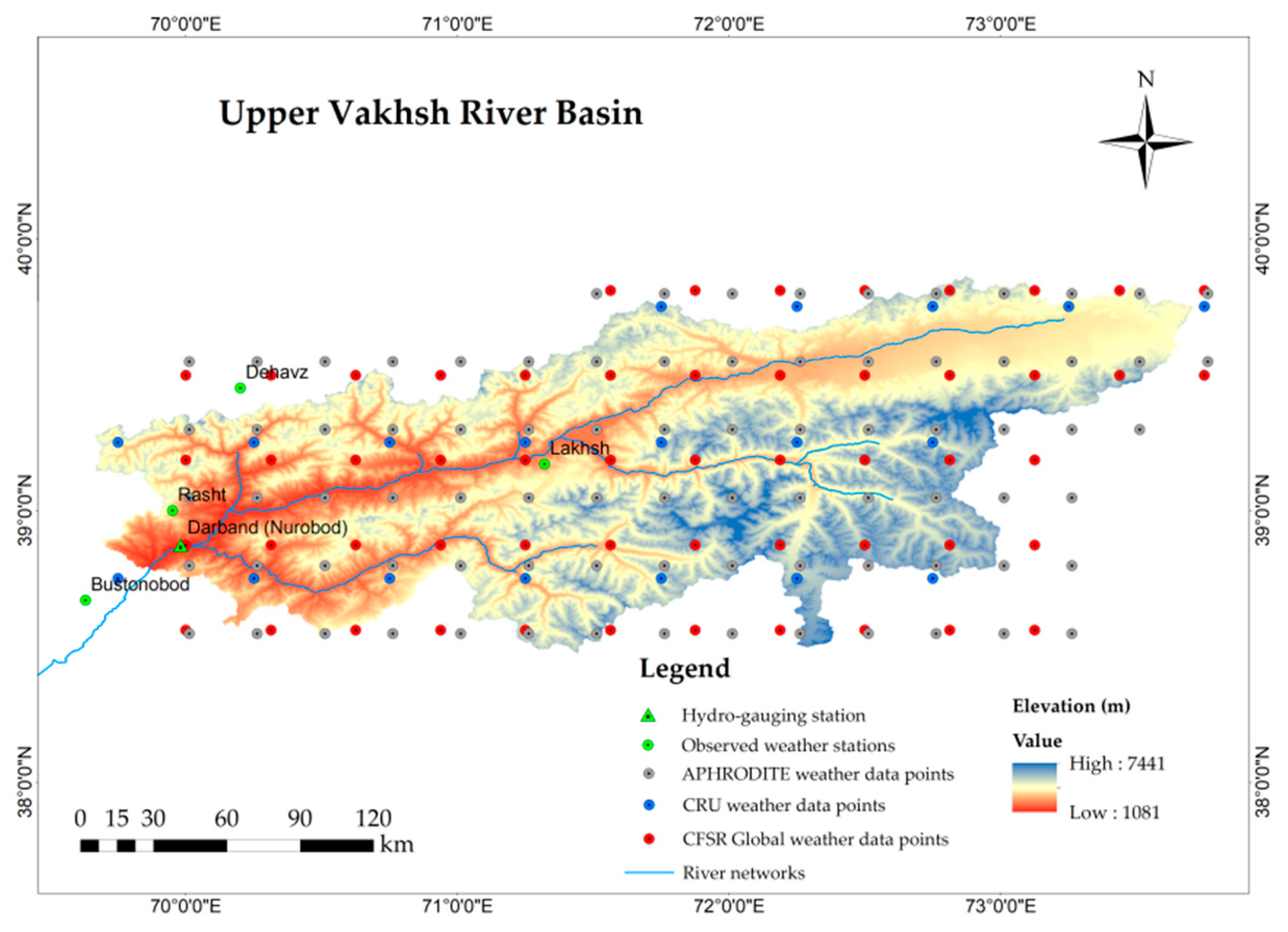
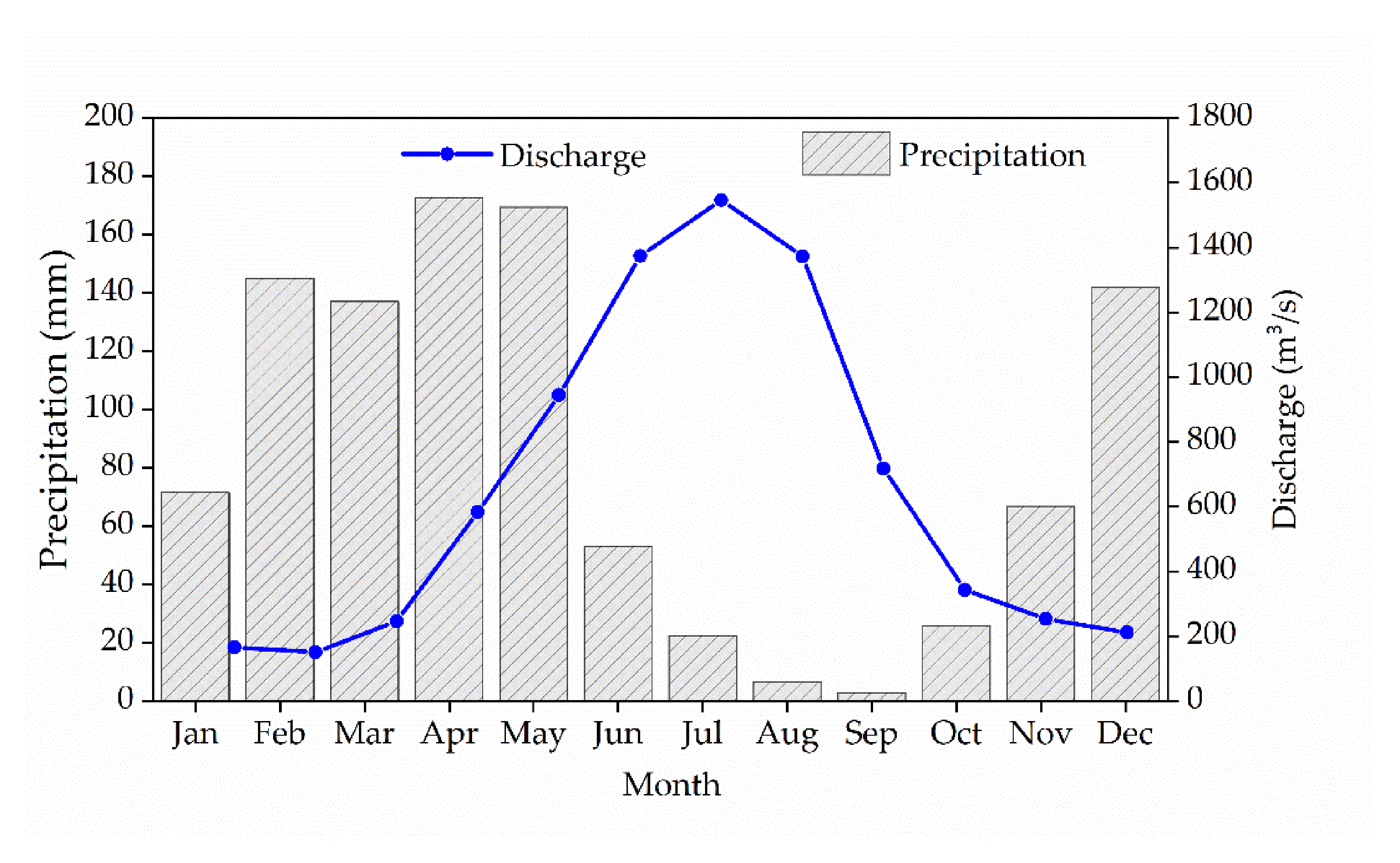
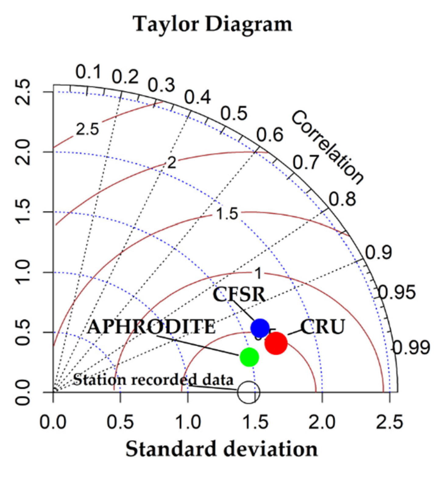
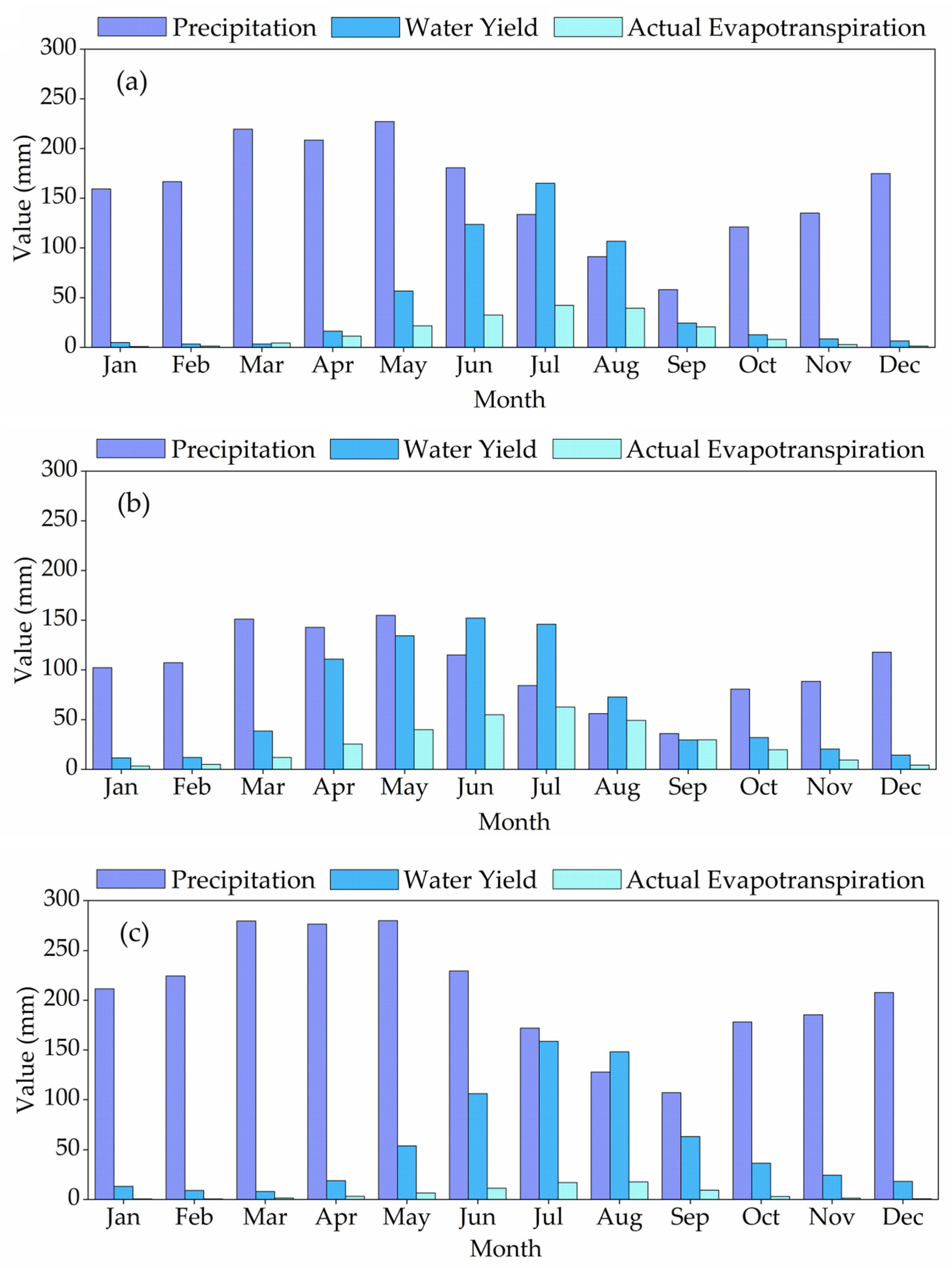

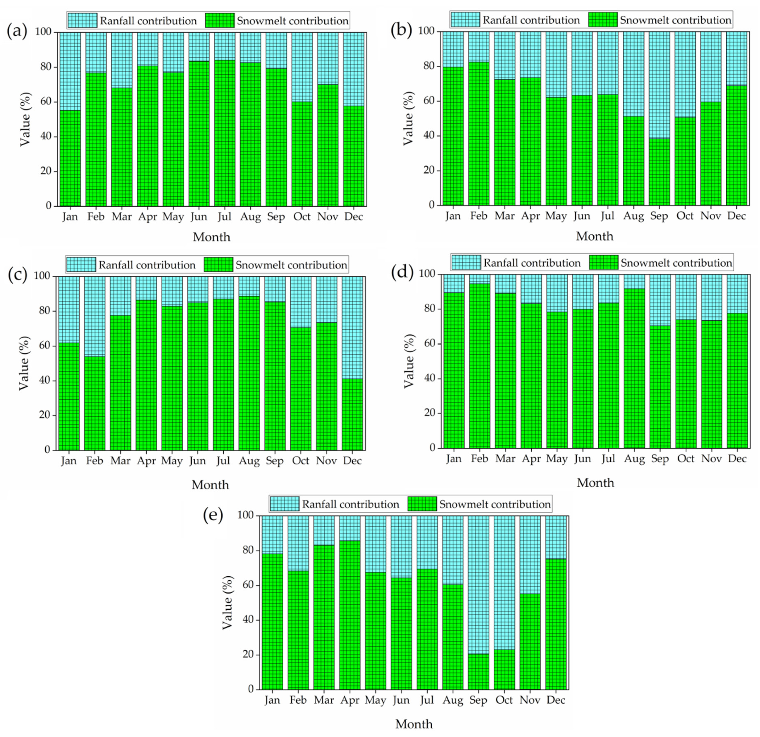
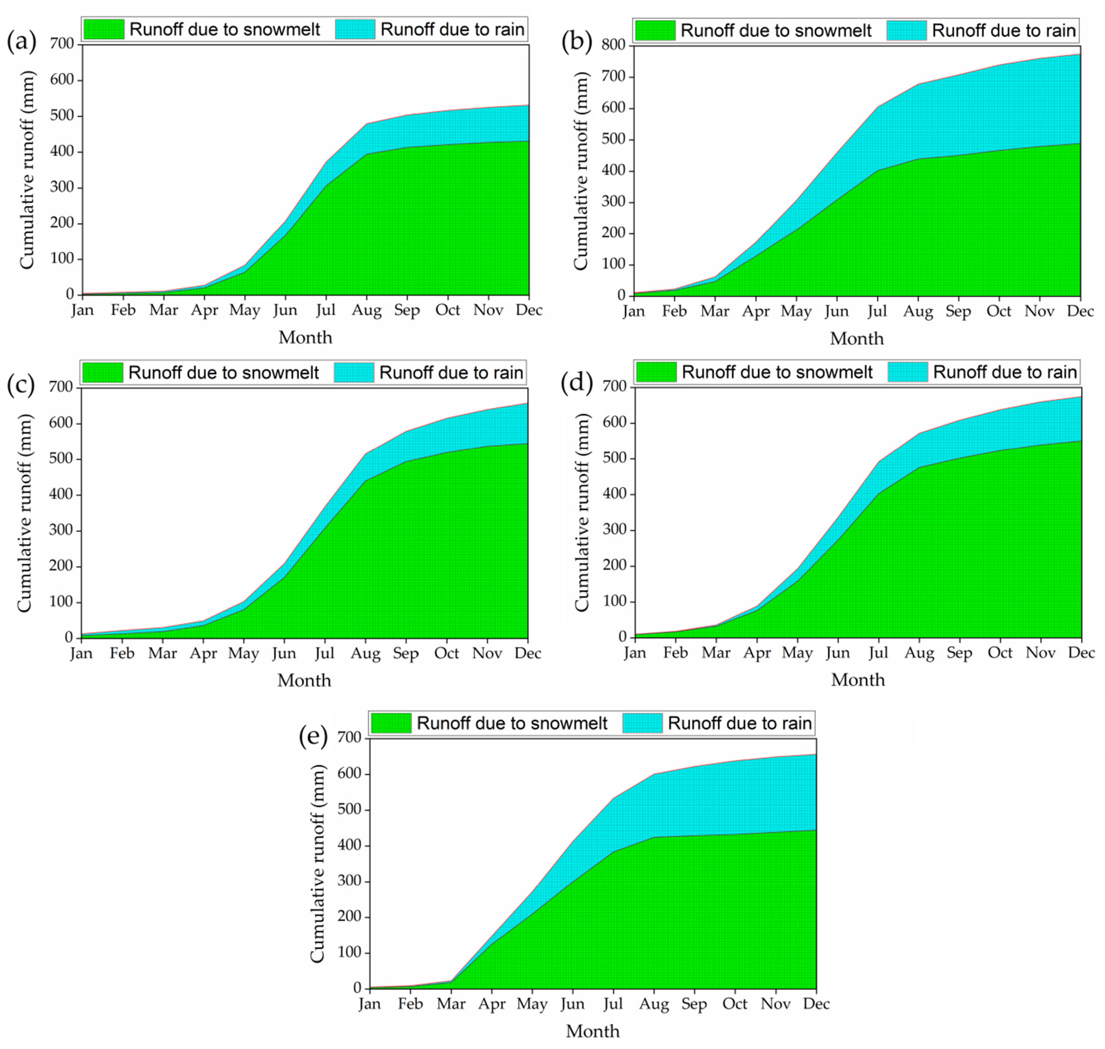
Publisher’s Note: MDPI stays neutral with regard to jurisdictional claims in published maps and institutional affiliations. |
© 2021 by the authors. Licensee MDPI, Basel, Switzerland. This article is an open access article distributed under the terms and conditions of the Creative Commons Attribution (CC BY) license (https://creativecommons.org/licenses/by/4.0/).