Abstract
The Sounding of the Atmosphere using Broadband Emission Radiometry (SABER) temperature measurements at low latitudes from 89 km to 97 km were used to derive the F10.7 and Ap index trends, and the trends were compared to model simulations. The annual mean nonzonal (e.g., at the model simulation location at 18° N, 290° E) SABER temperature showed a good-to-moderate correlation with F10.7, with a trend of 4.5–5.3 K/100 SFU, and a moderate-to-weak correlation with the Ap index, with a trend of 0.1–0.3 K/nT. The annual mean zonal mean SABER temperature was found to be highly correlated with the F10.7, with a similar trend, and moderately correlated with the Ap index, with a trend in a similar range. The correlation with the Ap index was significantly improved with a slightly larger trend when the zonal mean temperature was fitted with a 1-year backward shift in the Ap index. The F10.7 (Ap index) trends in the simulated O2 and the O(1S) temperature were smaller (larger) than those in the annual mean nonzonal mean SABER temperature. The trends from the simulations were better compared to those in the annual mean zonal mean temperature. The comparisons were even better when compared to the trend results obtained from fitting with a backward shift in the Ap index.
1. Introduction
Several studies have used airglow intensity or airglow temperature measurements to find trends in temperature [1,2,3,4,5,6]. These studies have focused on finding a linear trend or a solar trend using F10.7 as a proxy for solar cycle variation, since the solar radio flux at 10.7 cm (2800 MHz) is an excellent indicator of solar activity. The recent simulation studies by the authors of [7,8] showed that airglow intensities of OH(8,3), O2 atmospheric band, and O(1S) Greenline in the Mesosphere and Lower Thermosphere (MLT) region responded to the influences of the CO2 increase and the F10.7 and Ap index variations. In these studies, OH Chemistry Dynamics (OHCD) and Multiple-Airglow Chemistry Dynamics (MACD) airglow models [9,10,11,12] were used to simulate airglow response to the influences.
In Part 1 of this series by the authors of [13], the OHCD and the MACD model were used to simulate airglow intensity-weighted temperatures of the aforementioned airglow under the influence of the CO2 increase and F10.7 and Ap index variations from 1960 to 2019. Their simulation results were in agreement with the findings from other studies, i.e., solar response in temperature still remains one of the major sources of variations. The implication of this finding is that solar variations may interfere with the detection of human-induced temperature trends in the middle atmosphere [14,15]. In addition, their simulations also indicated that, due to the increase of CO2 gas concentration, the cooling trend would become more significant with time and would be detectable in the long-term observations if the increase of CO2 continues at a steady rate. A surprising result from these simulation studies was that airglow intensities and airglow temperatures in the MLT region also responded to geomagnetic activity (using the Ap index as a proxy since it provides a daily average level for geomagnetic activity) rather significantly.
To the best of our knowledge, none of the current trend studies that utilized observational data have examined the geomagnetic response of temperature in the MLT region. This provides us a strong motivation to examine whether an Ap index trend, in addition to an F10.7 trend, exists in the observational data. The Sounding of the Atmosphere using Broadband Emission Radiometry (SABER) onboard the Thermosphere Ionosphere Mesosphere Energetics Dynamics (TIMED) satellite has been measuring kinetic temperature since 2002. The remote sensing data provide a great opportunity for comparison with model simulations. In this work, SABER kinetic temperature data at the location of the model simulations (18° N, 290° E) were used for the trend analysis for the comparisons to the trend results obtained from the model simulations.
The paper is the Part 2 of the series “Trends in the Airglow Temperatures in the MLT Region” and is organized as follows. The data source for SABER kinetic temperature is described in Section 2. The results are presented in Section 3. The discussion is in Section 4 and the conclusions are in Section 5.
2. SABER Data
The SABER instrument onboard the NASA’s TIMED satellite has been routinely measuring kinetic temperature since 2002. The temperature was retrieved from the measurements of the CO2 emission at 15 um [16]. We used the level-2 temperature data which was downloaded from SABER’s website. The SABER kinetic temperature near the location of the model simulations (18° N, 290° E) was selected to find the annual mean temperature from 2002 to 2019. A bin size of 4 degrees in latitude and longitude (i.e., ±2°) and a bin size of 2 km (±1 km) in altitude were used. The SABER temperature error is estimated to be ~4 K (~2%) in the 80–100 km altitude range [17]. The error range is also listed on the SABER website. Given that the errors or uncertainties associated with the temperature were small, they should not affect the trend results derived from the temperature.
The authors of [13] simulated the airglow-intensity weighted OH(8,3), O2, and O(1S) temperatures for the aforementioned location to deduce the F10.7, Ap index, and CO2 trends in the simulated temperatures. Intensity-weighted temperature was obtained from the kinetic temperature weighted by airglow intensity [18], so the intensity-weighted temperature at peak height could be considered as kinetic temperature at that altitude. The SABER temperature data at 3 altitudes (89 km, 95 km, and 97 km) were selected for comparison to the OH(8,3), O2, and O(1S) intensity-weighted temperatures, respectively, from the Scenario 3 simulations by the authors of [13]. These airglow intensity-weighted temperatures are called airglow temperatures hereafter to be consistent with the terminology used in the Part 1 paper, i.e., OH temperature stands for OH airglow intensity-weighted temperature and so forth. The 3 altitudes were chosen because they are near the peak heights of the airglow emissions under consideration. Detailed information about the simulation results and the F10.7 and Ap index data sources used in this study can be found in the Part 1 paper [13]. The F10.7 values and Ap index values from 2002 to 2019 were taken from NASA’s website and the World Data Center for Geomagnetism at the Kyoto website, respectively. They were further averaged to produce the annual averages. Annual averages of the F10.7 and Ap index values were used in this study. Data sources for SABER, F10.7 and Ap index values can be found in the Acknowledgements.
3. Results
The annual mean SABER temperature data at the model simulation location was fitted with F10.7 or Ap index to find the trend. The SABER temperature at 89 km (axis on left, blue line with dots) and F10.7/Ap index (axis on right, red line for F10.7 and brown dashed line for Ap index) from 2002 to 2019 were plotted in Figure 1a. As can be seen, the SABER temperature overall displayed a variation similar to the F10.7 variation and loosely displayed the Ap index variation. The temperature data as a function of the F10.7 (in red dots) and of Ap index (in brown triangles), along with the fitting trend lines (red line denotes F10.7 trend and brown line denotes Ap index trend), were plotted in Figure 1b. The F10.7 and Ap index trends at 89 km were 5.29 ± 1.33 K/100 SFU, with R = 0.71, and 0.32 ± 0.12 K/nT, with R = 0.56, respectively, where R is the correlation coefficient. This indicates that the annual mean SABER temperature at 89 km had a moderate correlation with the F10.7 and a modest correlation with the Ap index. The simulated OH temperature taken from [13] had a low correlation with the F10.7 (−0.69 ± 0.28 K/100 SFU, R = 0.31) and a modest correlation with the Ap index (−0.12 ± 0.02 K/nT, R = 0.54). In addition, both the F10.7 and Ap index trends were negative.
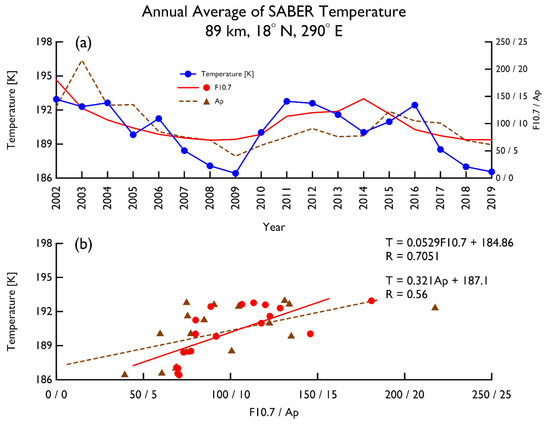
Figure 1.
Annual average of SABER temperature at 18° N, 290° E at 89 km. (a) Time series of temperature (blue line with dots), F10.7 (red line), and Ap index (brown dashed line). (b) Trend analysis of temperature as a function of the F10.7 (red line and dots) and of the Ap index (brown dashed line and triangles).
The SABER temperature (axis on left, blue line with dots) at 95 km and the F10.7/Ap index (axis on right, red line for F10.7 and brown dashed line for Ap index) as a function of year was plotted in Figure 2a, and the trend analysis results can be seen in Figure 2b. As the figure shows, the annual mean kinetic temperature at 95 km displayed a similar pattern of the F10.7 variation, but it was not as obvious with the Ap index variation. The SABER temperature at 95 km displayed good correlation with F10.7 with a trend of 5.23 ± 0.95 K/100 SFU (R = 0.81) and a modest correlation with the Ap index, with a trend of ~0.28 ± 0.1 K/nT (R = 0.56). The simulated O2 temperature taken from [13] showed a moderate correlation with the F10.7 (R = 0.61), with a smaller trend, 4.1 ± 0.7 K/100 SFU, and a very high correlation with the Ap index (R = 0.93), with a larger trend of ~0.6 ± 0.03 K/nT when compared to the SABER temperature.
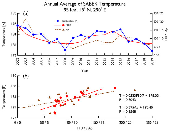
Figure 2.
Annual average of SABER temperature at 18° N, 290° E at 95 km. (a) Time series of temperature (blue line with dots), F10.7 (red line), and Ap index (brown dashed line). (b) Trend analysis of temperature as a function of the F10.7 (red line and dots) and of the Ap index (brown dashed line and triangles).
A similar plot for the SABER annual mean temperature at 97 km altitude is shown in Figure 3. We can see that the temperature in Figure 3a behaved similarly to the temperature at 95 km. The temperature variation roughly resembled the F10.7 variation and showed a trend of 4.49 ± 1.2 K/100 SFU, with a moderate R value of 0.68. It did not resemble the Ap index variation well, with a trend of 0.11 ± 0.12 K/nT, R = 0.23. The simulated O(1S) temperature, on the other hand, showed a weak correlation with F10.7, with a smaller trend of 2.0 ± 0.57 K/100 SFU (R = 0.42), and a strong correlation with Ap index, with a larger trend of ~0.41 ± 0.03 K/nT (R = 0.89). The trends from the model simulations and the SABER temperature measurements are placed side by side in Table 1 for easier inspection. Overall, the SABER temperature at the three altitudes displayed a good-to-moderate correlation with the F10.7, with a trend in the range of 3.29–6.62 K/100 SFU centered around 5 K/100 SFU. The Ap index trend in the region between 89 km and 95 km, excluding the trend at 97 km because of its low correlation, showed a trend in the range of 0.2–0.4 K/nT centered around 0.3 K/nT.
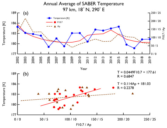
Figure 3.
Annual average of SABER temperature at 18° N, 290° E at 97 km. (a) Time series of temperature (blue line with dots), F10.7 (red line), and Ap index (brown dashed line). (b) Trend analysis of temperature as a function of the F10.7 (red line and dots) and of the Ap index (brown dashed line and triangles).

Table 1.
F10.7 and Ap index trends with correlation coefficient R obtained from the simulated airglow temperatures and annual mean SABER temperature measurements at 18° N, 290° E.
Admittedly, the model simulation values from [13] do not compare that well to the values using the annual mean nonzonal SABER temperature as shown in Table 1. The authors of [13] intentionally did not include dynamics in the model simulations so that they could better assess the influences of solar variation, geomagnetic activity, and CO2 increase on the airglow temperatures. In that regard, perhaps a better comparison between the model simulations and observations would be to use the results from the zonal mean SABER temperature. It would also be interesting to see how the trends in the SABER temperature could change when the temperature is zonally averaged to minimize the dynamical influences from gravity waves, planetary waves, or tides.
Similar plots as those in Figure 1a,b are shown in Figure 4a,b using the zonal mean SABER temperature at 89 km. Comparing Figure 1a and Figure 4a, we can see that the zonal mean data resembled the F10.7 variation much better, as also indicated by the correlation coefficient of R = 0.90 in Figure 4b in comparison to R = 0.71 in Figure 1b. However, the F10.7 trend in the zonally averaged data was found to be 3.95 ± 0.49 K/100 SFU, which is smaller than the F10.7 trend in Figure 1b. As for the Ap index trend, the zonally averaged data showed a slightly larger correlation coefficient R = 0.6 and a smaller Ap index trend of ~0.2 ± 0.07 K/nT when compared to the values in Figure 1b.
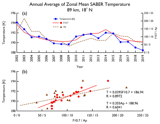
Figure 4.
Zonal mean annual average of SABER temperature at 18° N at 89 km. (a) Time series of temperature (blue line with dots), F10.7 (red line), and Ap index (brown dashed line). (b) Trend analysis of temperature as a function of the F10.7 (red line and dots) and of the Ap index (brown dashed line and triangles).
Figure 5a shows the annual mean zonally averaged SABER temperature at 95 km and Figure 5b shows the trend analysis results. Comparing Figure 5a to Figure 2a, we can see that the zonal mean data at 95 km also resembled the F10.7 variation better, showing a higher correlation (R = 0.93). Both data in Figure 2b and Figure 5b showed an almost the same F10.7 trend ~5.2 K/100 SFU. As for Ap index trend, the trends in Figure 5b and Figure 2b did not show any significant difference. Both datasets had a similar Ap index trend in the range of 0.25–0.28 K/nT and a similar R value (0.56–0.58).
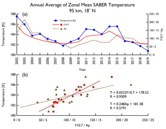
Figure 5.
Zonal mean annual average of SABER temperature at 18° N at 95 km. (a) Time series of temperature (blue line with dots), F10.7 (red line), and Ap index (brown dashed line). (b) Trend analysis of temperature as a function of the F10.7 (red line and dots) and of the Ap index (brown dashed line and triangles).
Figure 6a,b show the time series of the zonally averaged annual mean SABER temperature at 97 km and the trend results, respectively. Comparing Figure 6a to Figure 3a, we can see that the zonal mean temperature better resembled both the F10.7 and Ap index variation. Regarding the trend values at 97 km, the zonal mean and nonzonal mean data showed a similar F10.7 trend, 4.9 K/100 SFU for the former and 4.5 K/100 SFU for the latter, but the correlation coefficient was much higher (R = 0.92) for the zonal mean data. As for the Ap index trend, the zonal mean temperature had a larger value (0.23 K/nT) and a better correlation (R = 0.56) than the values using the nonzonal mean temperature. The trend analysis results of the annual mean zonal mean SABER temperature at the three altitudes are listed in Table 2.
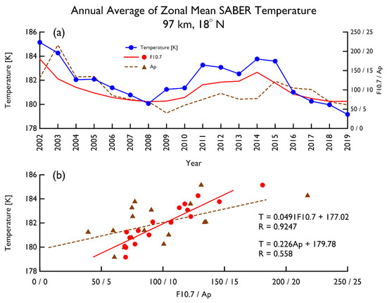
Figure 6.
Zonal mean annual average of SABER temperature at 18° N at 97 km. (a) Time series of temperature (blue line with dots), F10.7 (red line), and Ap index (brown dashed line). (b) Trend analysis of temperature as a function of the F10.7 (red line and dots) and of the Ap index (brown dashed line and triangles).
Table 2.
F10.7 and Ap index trends with correlation coefficient R obtained from the zonal mean SABER temperature measurements.
A better correlation with F10.7 and Ap index is seen in the zonal mean temperature data for all three altitudes. At 89 km, both the F10.7 and Ap index trends in the zonal mean data were smaller than the trends in the nonzonal mean data. A better correlation with F10.7 is seen in the zonal mean data, whereas the zonal mean and nonzonal mean data had a similar degree of correlation with Ap index. At 95 km, the zonal and nonzonal mean temperature showed similar F10.7 and Ap index trends. The F10.7 trends at 97 km were similar but the Ap index trend in the zonal mean temperature was larger. When we compare the trends in the zonal mean SABER temperature to the trends in the model simulated O2 and O(1S) temperatures, we can see that the zonal mean SABER temperature at 97 km showed an Ap index trend value closer to that in the simulated O(1S) temperature.
4. Discussion
The simulated OH temperature showed a much smaller and negative F10.7 trend and a negative Ap index trend, whereas the annual mean nonzonal SABER temperature at the OH peak height showed positive trends, as shown in Table 1. The F10.7 and Ap index trends were smaller in the zonal mean temperature, as shown in Table 2 and Table 3. Admittedly, the results at the OH airglow peak altitude from satellite measurements and simulations do not agree. The reason is that, as discussed by the authors of [13], “the F10.7 and Ap variations have not been carried below 110 and 90 km, respectively” [19]. The authors of [13] used the OHCD model, which employed the Naval Research Laboratory Mass Spectrometer and Incoherent Scatter Radar-00 (NRLMSISE-00) empirical model, as their reference model in their simulation work. If the F10.7 and Ap index variations are not carried explicitly below the airglow altitudes in the reference model, airglow models such as the OHCD model will only be able to simulate temperature variation induced by the F10.7 or Ap index variation that is inherently embedded in the data used by the empirical model.
Table 3.
F10.7 and Ap index trends with correlation coefficient R obtained from the zonal mean SABER temperature measurements fitted with 1-year shift in the Ap index.
In various degrees, the temperature measurements at the three altitudes used in this study all displayed that the temperature variation generally resembled the F10.7 variation. It also resembled the Ap index variation but to a lesser degree. The atmospheric response to solar input might take up to several years [20], and it has been reported that a phase difference (time-lag) might exist between solar input and solar response which can affect the magnitude of the solar response coefficient [20,21]. It was found that the correlation would be improved when a time lag was applied to the datasets (Holmen et al., 2014). Since F10.7 and Ap index are correlated (see the discussion in Part 1 of the series by the authors of [13] and also [22]), it is plausible that a time lag also exists between the temperature and Ap index if a time lag exists between the temperature and F10.7.
We noticed that there seemed to be a 1-year time lag in some years between the SABER temperature and Ap index and that the Ap index variation preceded the temperature variation. Therefore, we also did a trend analysis with a 1-year shift in Ap index but kept the time series of annual mean zonal mean SABER temperature intact to see if the correlation of Ap index with the temperature would improve. We list the trend analysis results for the three altitudes in Table 3 and only show the results for 95 km in Figure 7. Figure 7a shows the annual mean zonal mean SABER temperature at 95 km (axis on left) and F10.7 and Ap index (axis on right) with Ap index being shifted 1 year backward, i.e., the original Ap index value in 2003 is now the value for 2002, the original value in 2004 is now the value for 2003, and so forth. Comparing Figure 5a and Figure 7a, we can see that the annual mean zonal mean SABER temperature variation resembled the Ap index variation much better, as shown in Figure 7a. Figure 7b displays the trend analysis results, showing a much higher correlation with Ap index when the Ap index was shifted 1 year backward. The correlation coefficient between the temperature and the shifted Ap index changed from R = 0.58 (in Figure 5b) to R = 0.82. The significant improvement in the correlation when there was a 1-year shift in Ap index was also seen for the 89 km and 97 km altitude.
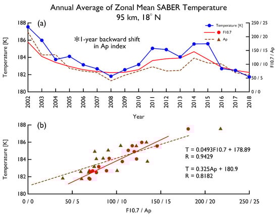
Figure 7.
Annual average of zonal mean SABER temperature at 18° N at 95 km with the Ap index shifted 1 year backward. (a) Time series of temperature (blue line with dots), F10.7 (red line), and Ap index (brown dashed line). (b) Trend analysis of temperature as a function of the F10.7 (red line and dots) and of the Ap index (brown dashed line and triangles).
When we examine the values in Table 3 and compare them to the values in Table 2, several things are noted: (1) The annual mean zonal mean SABER temperature at the three altitudes in Table 3 all had a strong correlation with both the F10.7 and Ap index, as indicated by the high R values. (2) The F10.7 trend values in Table 3 were about ~6–7% lower but remained close to the values in Table 2 for all three altitudes. Note that the correlation between the annual mean zonal mean SABER temperature and F10.7 was slightly different from the correlation coefficients in Table 2 because the fitting data range was 1 year shorter. (3) The Ap index trends in Table 3 were ~30% larger than the values in Table 2 for all three altitudes and showed a much stronger correlation. These results indicate that annual mean zonal mean SABER temperature was highly correlated with Ap index when the Ap index was shifted 1 year backward. We should note that even without the shift in Ap index, the temperature also demonstrated a moderate correlation with Ap index. Another thing to be noted is that such time lag was not seen in the model-simulated airglow temperatures by Huang and Vanyo (2020) [13]. The cause for the time delay of SABER temperature response to geomagnetic activity, if it is real, is still unknown and is beyond the scope of the current study. It is hoped that our study will bring this to the attention of the scientific community for further investigation.
When we compared the trend results from [13] to the results from the annual mean zonal mean SABER temperature without a shift in Ap index, we noted that the F10.7 (Ap index) trends were larger (smaller) in SABER temperature at the O2 and O(1S) peak heights. Comparing the simulation results to the results obtained from the temperature fitted with a 1-year shift in the Ap index, we found that the Ap index trends in the annual mean zonal mean SABER temperature became larger and closer to the Ap index trends from the simulations at the O2 and O(1S) peak heights.
Since this paper is focused on finding trends in the temperature induced by the influence of solar variations and geomagnetic activity, annual averaged values should be used. We notice that the day-to-day variability of geomagnetic activity was more variant than that of solar variation, so a question might arise as to whether the annual averaged Ap index values should be used. However, we are looking at the trends on a much larger timescale rather than on the daily basis, so the annual averaged values of Ap index should be used. This is supported by our results, which show that geomagnetic activity affects the temperature in a way that can be quantified by a trend line, with a correlation coefficient that should not be dismissed. In addition, since the F10.7 and Ap index are closely correlated (please see the discussion in Part 1 and in this paper), it is justified to look at the trend caused by the annual mean values of the Ap index. How the temperature responds to the daily variability of geomagnetic activity is an interesting subject but is beyond the scope of this paper.
Note that the model simulations were for a fixed location at (18° N, 290° E), so the trend results are valid only for that location. The trend results may not apply to other locations at different latitudes and longitudes. It would be interesting to examine the trends at other locations to better understand the differences due to the use of different locations, but this will be conducted in a future study. Regarding the use of airglow intensity-weighted temperatures, we agree that the selected SABER temperature is not weighted by the airglow intensities at the three altitudes, but the simulated airglow temperatures are intensity weighted. As we mentioned earlier in Section 2, the intensity-weighted temperatures were obtained using the kinetic temperature weighted by intensity, so the intensity-weighted temperature should be close to the kinetic temperature at the peak height. We note that there was a broad range of altitude overlap for O2 and O(1S) emission layers. However, the intensity-weighted temperature at the respective peak height would still dominate, it can therefore represent the temperature at its respective peak height.
5. Conclusions
Annual mean nonzonal mean SABER temperature at low latitude near the model simulation location at (18° N, 290° E) was analyzed to find the F10.7 and Ap index trends at three altitudes (89 km, 95 km, and 97 km). The temperatures at the three altitudes showed a good-to-moderate correlation with the F10.7, with a correlation coefficient R value in the range of 0.7–0.8, and a moderate-to-weak correlation with the Ap index, with the R value in the range of 0.2–0.6. The temperature showed a F10.7 (Ap index) trend in the range of 4.5–5.3 K/100 SFU (0.1–0.3 K/nT) in the altitude range of interest.
We also analyzed the annual mean zonal mean SABER temperature and found that it showed a much better correlation with F10.7 for all three altitudes, with a F10.7 trend in the range of 4.0–5.2 K/100 SFU. We also found a better correlation with the Ap index for all three altitudes, with an Ap index trend in the range of 0.2–0.25 K/nT. We further experimented with the trend analysis by fitting the annual mean zonal mean temperature with a 1-year shift in Ap index. The results obtained all displayed an even higher correlation with both the F10.7 and Ap index. The F10.7 trend was in the range of 3.7–4.6 K/100 SFU and the Ap index trend was in the range of 0.26–0.31 K/nT.
Comparing the trends from annual mean nonzonal mean SABER temperature to those from [13], it was found that the F10.7 (Ap index) trend in the SABER temperature was about 1 K/100 SFU (0.3 K/nT) larger (smaller) than the trend in the simulated O2 temperature. Comparing to the simulated O(1S) temperature, the annual mean nonzonal mean SABER temperature had a larger F10.7 trend, with a difference of ~2.5 K/100 SFU between the F10.7 trends, and a smaller Ap index trend, with a difference of ~0.3 K/nT. The trends in the simulated OH temperature and those in the SABER temperature at 89 km do not agree. The simulated OH temperature showed an anticorrelation with the F10.7 and Ap index, while the SABER temperature showed a F10.7 trend of 5.3 K/100 SFU and an Ap index trend of 0.3 K/nT.
Based on these values, it is noted that the model simulations by the authors of [13] for O2 and O(1S) temperatures compare better with the trends obtained from the annual mean zonal mean SABER temperature than with the results obtained from the nonzonal mean SABER temperature, and they compare even better with the trends when the temperature was fitted with a 1-year shift in the Ap index. Our trend results using satellite measurements and the trends from model simulations reported in Part 1 of the series indicate that temperature in the MLT region is correlated with the F10.7 and Ap index, suggesting that both the solar variation and geomagnetic activity play a role in temperature variation.
Author Contributions
Conceptualization, T.-Y.H.; Formal analysis, T.-Y.H. and M.V.; Funding acquisition, T.-Y.H.; Investigation, T.-Y.H. and M.V.; Methodology, T.-Y.H.; Project administration, T.-Y.H.; Resources, T.-Y.H.; Software, M.V.; Writing—original draft, T.-Y.H. All authors have read and agreed to the published version of the manuscript.
Funding
This research was funded by US NSF AGS-1903346 to The Pennsylvania State University.
Institutional Review Board Statement
Not applicable.
Informed Consent Statement
Not applicable.
Data Availability Statement
Annual averages of the zonal mean and non-zonal mean SABER temperature data and simulated airglow temperatures can be accessed here, Processed Data.
Acknowledgments
T.-Y.H. and M.V. acknowledge support from the US NSF AGS-1903346 to The Pennsylvania State University. SABER temperature level 2 data was downloaded from http://saber.gats-inc.com/. F10.7 is from the NASA website (http://omniweb.gsfc.nasa.gov/form/dx1.html) and Ap index is from the World Data Center for Geomagnetism, Kyoto website (http://wdc.kugi.kyoto-u.ac.jp/kp/).
Conflicts of Interest
The authors declare no conflict of interest. The funders had no role in the design of the study; in the collection, analyses, or interpretation of data; in the writing of the manuscript, or in the decision to publish results.
References
- Scheer, J.; Reisin, E.R.; Mandrini, C.H. Solar activity signatures in mesopause region temperatures and atomic oxygen related airglow brightness at El Leoncito, Argentina. J. Atmos. Sol. Terr. Phys. 2005, 67, 145–154. [Google Scholar] [CrossRef]
- Pertsev, N.; Perminov, V. Response of the mesopause airglow to solar activity inferred from measurements at Zvenigorod, Russia. Ann. Geophys. 2008, 26, 1049–1056. [Google Scholar] [CrossRef]
- Das, U.; Pan, C.J.; Sinha, H.S.S. Effects of solar cycle variations on oxygen green line emission rate over Kiso, Japan. Earth Planets Space 2011, 63, 941–948. [Google Scholar] [CrossRef]
- Hall, C.M.; Dyrland, M.E.; Tsutsumi, M.; Mulligan, F.J. Temperature trends at 90 km over Svalbard, Norway (78° N 16° E), seen in one decade of meteor radar observations. J. Geophys. Res. 2012, 117, D08104. [Google Scholar] [CrossRef]
- Holmen, S.E.; Dyrland, M.E.; Sigernes, F. Long-term Trends and the Effect of Solar Cycle Variations on Mesospheric Winter Temperatures over Longyearbyen, Svalbard (78° N). J. Geophys. Res. Atmos. 2014, 119, 6596–6608. [Google Scholar] [CrossRef]
- Kalicinsky, C.; Knieling, P.; Koppmann, R.; Offermann, D.; Steinbrecht, W.; Wintel, J. Long-term Dynamics of OH* Temperatures over Central Europe: Trends and Solar Correlations. Atmos. Chem. Phys. 2016, 16, 15033–15047. [Google Scholar] [CrossRef]
- Huang, T.-Y. Simulations of Airglow Variations Induced by the CO2 Increase and Solar Cycle Variation from 1980 to 1991. J. Atmos. Sol. Terr. Phys. 2016, 147, 138–147. [Google Scholar] [CrossRef]
- Huang, T.-Y. Influences of CO2 Increase, Solar Cycle Variation, and Geomagnetic Activity on Airglow from 1960 to 2015. J. Atmos. Sol. Terr. Phys. 2018, 171, 164–175. [Google Scholar] [CrossRef]
- Huang, T.-Y.; Hickey, M.P. On the latitudinal variations of the non-periodic response of minor species induced by a dissipative gravity-wave packet in the MLT region. J. Atmos. Sol. Terr. Phys. 2007. [Google Scholar] [CrossRef]
- Huang, T.-Y.; Hickey, M.P. Secular variations of OH nightglow emission and of the OH intensity-weighted temperature induced by gravity-wave forcing in the MLT region. Adv. Space Res. 2008. [Google Scholar] [CrossRef]
- Huang, T.-Y.; George, R. Simulations of Gravity Wave-induced Variations of the OH(8,3), O2(0,1), and O(1S) Airglow Emissions in the MLT Region. J. Geophys. Res. Space Phys. 2014, 119. [Google Scholar] [CrossRef]
- Amaro-Rivera, Y.; Huang, T.-Y.; Urbina, J.; Vargas, F. Empirical Values of Branching Ratios in the Three-Body Recombination Reaction for O(1S) and O2(0,0) airglow chemistry. Adv. Space Res. 2018, 62, 2679–2691. [Google Scholar] [CrossRef]
- Huang, T.Y.; Vanyo, M. Trends in the Airglow Temperatures in the MLT Region—Part 1: Model Simulations. Atmosphere 2020, 11, 468. [Google Scholar] [CrossRef]
- Beig, G.; Scheer, J.; Mlynczak, M.G.; Keckhut, P. Overview of the temperature response in the mesosphere and lower thermosphere to solar activity. Rev. Geophys. 2008, 46, RG3002. [Google Scholar] [CrossRef]
- Beig, G. Long-term Trends in the Temperature of Mesosphere/Lower Thermosphere Region: 2. Solar Response. J. Geophys. Res. 2011, 116, A00H12. [Google Scholar] [CrossRef]
- Mertens, C.J.; Mlynczak, M.G.; López-Puertas, M.; Wintersteiner, P.P.; Picard, R.H.; Winick, J.R.; Gordley, L.L.; Russell, J.M. Retrieval of mesospheric and lower thermospheric kinetic temperature from measurements of CO2 15 μm Earth Limb Emission under non-LTE conditions. Geophys. Res. Lett. 2001, 28, 1391–1394. [Google Scholar] [CrossRef]
- Xu, J.; She, C.Y.; Yuan, W.; Mertens, C.; Mlynczak, M.; Russell, J. Comparison between the temperature measurements by TIMED/SABER and lidar in the midlatitude. J. Geophys. Res. 2006, 111, A10S09. [Google Scholar] [CrossRef]
- Huang, T.-Y. Gravity Waves-induced Airglow Temperature Variations, Phase Relationships, and Krassovsky Ratio for OH(8,3) Airglow, O2(0,1) Atmospheric Band, and O(1S) Greenline in the MLT Region. J. Atmos. Sol. Terr. Phys. 2015, 130, 68–74. [Google Scholar] [CrossRef]
- Hedin, A.E. Extension of the MSIS thermosphere model into the middle and lower thermosphere. J. Geophys. Res. 1991, 96, 1159–1172. [Google Scholar] [CrossRef]
- Wynn, T.A.; Wickwar, V.B. The Effects of Model Misspecification on Linear Regression Coefficients as Applicable to Solar and Linear Terms. Available online: https://digitalcommons.usu.edu/atmlidar_rep/3/ (accessed on 15 May 2020).
- French, W.J.R.; Klekociuk, A.R. Long-term trends in Antarctic winter hydroxyl temperatures. J. Geophys. Res. 2011, 116, D00P09. [Google Scholar] [CrossRef]
- Verbanac, G.; Vrsnak, B.; Temmer, M.; Mandea, M.; Korte, M. Four decades of geomagnetic and solar activity: 1960–2001. J. Atmos. Sol. Terr. Phys. 2010, 72, 607–616. [Google Scholar] [CrossRef]


Publisher’s Note: MDPI stays neutral with regard to jurisdictional claims in published maps and institutional affiliations. |
© 2021 by the authors. Licensee MDPI, Basel, Switzerland. This article is an open access article distributed under the terms and conditions of the Creative Commons Attribution (CC BY) license (http://creativecommons.org/licenses/by/4.0/).