Methane Emissions during the Tide Cycle of a Yangtze Estuary Salt Marsh

Abstract

Methane (CH₄) emissions from estuarine wetlands were proved to be influenced by tide movement and inundation conditions notably in many previous studies. Although there have been several researches focusing on the seasonal or annual CH₄ emissions, the short-term CH₄ emissions during the tide cycles were rarely studied up to now in this area. In order to investigate the CH₄ emission pattern during a tide cycle in Yangtze Estuary salt marshes, frequent fixed-point observations of methane flux were carried out using the in-situ static closed chamber technique. The results indicated that the daily average CH₄ fluxes varied from 0.68 mgCH₄·m⁻²·h⁻¹ to 4.22 mgCH₄·m⁻²·h⁻¹ with the average flux reaching 1.78 mgCH₄·m⁻²·h⁻¹ from small tide to spring tide in summer. CH₄ fluxes did not show consistent variation with both tide levels and inundation time but increased steadily during almost the whole research period. By Pearson correlation analysis, CH₄ fluxes were not correlated with both tide levels (R = −0.014, p = 0.979) and solar radiation (R = 0.024, p = 0.865), but significantly correlated with ambient temperature. It is temperature rather than the tide level mainly controlling CH₄ emissions during the tide cycles. Besides, CH₄ fluxes also showed no significant correlation with the underground pore-water CH₄ concentrations, indicating that plant-mediated transport played a more important role in CH₄ fluxes compared with its production and consumption.

1. Introduction

Methane (CH₄) ranks second to carbon dioxide (CO₂) as an important greenhouse gas (GHG) without considering water vapor [1]. The single kilogram radiation effect of atmospheric CH₄ is 34 times stronger than that of atmospheric CO₂ over a 100-year time scale [2] and the current estimation of the warming potential of CH₄ may be 10–40% lower than if its chain effects on aerosols and other chemical compounds in the atmosphere were included [3]. Therefore, a small change in atmospheric CH₄ concentration implies significant changes for the future climate [2]. Wetlands are the single biggest CH4 source type, driven by their sufficient sediment organic carbon (SOC) supply and a strict anaerobic environment [4,5,6]. It is estimated that wetlands contribute more than 30% of the total CH₄ emissions globally with anthropogenic emissions such as livestock, landfills, waste management, fossil fuel production and rice paddies constituting most of the rest of CH₄ emissions [7,8].

Wetland CH₄ emission is a very complex process under the comprehensive effects of the environmental factors, including inundation conditions [9], carbon availability [5], temperature [10], salinity [11] and vegetation [12]. The above environmental factors mainly influence CH₄ production and emission via changing the redox status, the microbial activity, the substrate concentration and also the emission pathways. The specific production and emission mechanism may differ a lot between tidal and non-tidal wetlands. The first major reason for this is that the much higher sulfate concentrations in tidal wetlands allows sulfate-reducing bacteria to outcompete methanogenic communities for electron donors [13]. Thus, as a proxy for sulfate availability, sediment salinity is proved to be closely related with CH₄ production in tidal wetlands [11,14]. Another obvious difference between tidal and non-tidal wetlands is tide movement, which can change the inundation condition for CH₄ production. Up to now, very few case studies focused on the sediment–air and also the sediment–water CH₄ emission characteristics during the tide movement, although the water–air interface was systematically investigated along a gradient of the subtropical Brisbane River estuary [15]. As a matter of fact, the inundation time of salt marsh sediment is much less than its exposure time in Yangtze Estuary. Thus, the investigation of CH₄ emissions across the sediment–air interface is also necessary to estimate the wetland CH₄ sources.

CH₄ generated underground rises upward to wetland surface in three ways, including molecular diffusion, bubble ebullition and aquatic plant transportation [12,16,17,18]. The migration process could cause the majority of CH₄ to be oxidized by both aerobic and anaerobic oxidation [19,20]. The final CH₄ exchange flux between wetland and atmosphere was decided by the comprehensive actions of production, consumption and transportation [21,22,23]. Any environmental factor that could influence the above three processes will be able to determine CH₄ emission flux. For instance, as an important environmental factor controlling various biogeochemical processes, temperature also greatly influences both CH₄ production and emissions. On the one hand, activity of methanogenic bacteria in the anoxic environment increases with temperature, which could lead to the continuous accumulation of CH₄ in sediment pore water. On the other hand, the concentration-driven molecular diffusion is the main mechanism of plant transportation for CH₄, which could be greatly improved by a temperature increase. The Yangtze estuary, located in a subtropical area with a clear four seasons, is one of the biggest estuaries in the world. Previously, several researches were carried out to investigate the seasonal and even interannual variations of CH₄ emissions [23,24]. However, the variation characteristic of CH₄ emissions during a tide cycle in the relatively shorter time scale was rarely studied. Therefore, the main objectives of this study were to (1) identify the short-term CH4 emission patterns during the tide cycles; (2) examine the relationship between CH₄ emissions and pore-water CH₄ concentrations; and (3) distinguish the main driving factors of the short-term variation of CH₄ flux among the environmental factors we observed.

2. Methods and Materials

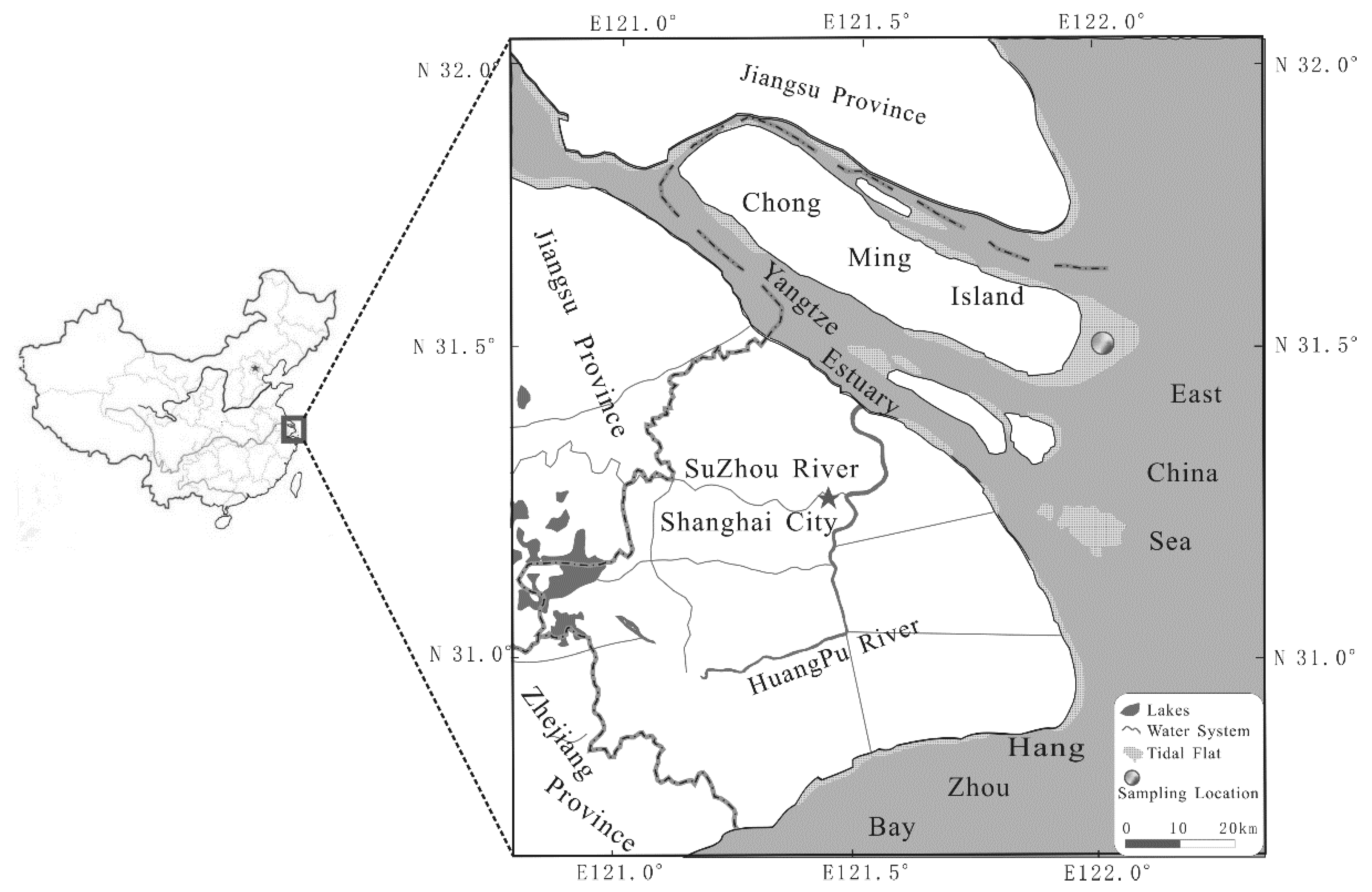
2.1. Study Sites

The Yangtze estuary, located in East Asia with a subtropical monsoon climate, is one of the three largest estuaries in the world. The tidal pattern in the Yangtze estuary is characterized as mixed semi-diurnal tide and there are two floods and ebbs with different heights each day [9]. On a monthly scale, there are two spring tides and two neap tides as a result of the periodic motion of the moon. Although the tide water could rise to the high tidal flat when the spring tide occurs, this does not mean a long inundation time for the estuary salt marsh sediment because the highest tidal range between the high and low tides accelerate the tide water movement. Similarly, the longest inundation time also does not happen in the neap tide period because even the height of high-tide, it cannot reach the salt marsh. So the longest inundation condition of the salt marsh appears between the neap and spring tide.

Our study site is located on the eastern coast of Chongming island, which is the most complete and best-protected natural wetland, having not been disturbed too much by human activity in the Yangtze estuary (see Figure 1). The region has an irregular semidiurnal tide and the annual maximum and average tidal ranges are 4.89 m and 2.7 m, respectively [25]. With the natural sediment deposition for many years, the eastern Chongming island well developed high, middle and low tidal flats with the dominant species of Phragmites australis in the high tidal flat and Scirpus mariqueter in the middle tidal flat. There is no vegetation in the low tidal flat, where the sediment mainly consists of sandy particles. Our study focused on the middle flat where methanogenesis was greatest among the three geomorphic types. Scirpus mariqueter is the endemic species in the Yangtze estuary and it is also the pioneer species coming along with the natural seaward extension of the tidal flat. Its growing season is from April to October and the biomass achieved the maximum in August [26,27].

2.2. Gas Sampling and Measurement

The common in-situ static (non-steady state non-flow through) closed chamber technique was selected to perform flux measurement [24]. The chamber was composed of two parts: a collar base and a chamber cover used to collect gas samples. The base is 5 cm in height with a 30 cm inner diameter and has a 3 cm height and a 1.5 cm width U-shaped groove, and is made from a 1 mm stainless steel sheet. Because of the tide cycles, if the base was previously installed in the marsh, there would be much sediment settling down in the base. Therefore, we sharpened the blade of the end of the base to make sure it could cut into the sediment with little disturbance. Both transparent and opaque chambers were set when sampling. Fluxes in opaque chambers were considered as the nightly fluxes. Transparent chambers were made of 3 mm thickness acrylic cylinder and the opaque chambers were made of a 0.4 mm thick iron sheet covered by an insulating layer and aluminum foil to reduce heat transmission and sunlight reflection. The exact dimensions of the chamber are 50 cm height and 30 cm inner diameter. A small electric fan and a kerosene thermometer were installed inside the chamber. The fan is used to blend the air in the chamber and the thermometer is used to measure the sampling-end temperature in the chamber. Besides, a balance pipe was used to equalize the inner–outer air pressure [24]. Every chamber was installed with a polyethylene pipe on its top for sampling and a clinical three-way valve was connected to the end of the pipe. All the connections and gaps were sealed by silicon rubber to keep the chambers air tight. On each sampling day, the bases were installed on the sediment surface about 0.5 h before sampling, and then chambers were fixed on the base and sealed by water in the U-shaped collar base.

The gas samplings were carried out at low tides during daytime at two-day intervals from 10 to 24 July, 2011 in the summer. Most of the samplings began at 6:00 am and ended at 4:30 pm, except for the delayed sampling at 7:30 am on 16th July and 19th July because of slow walking in tide water brought about by the spring tide. Immediately after installing each chamber and again after 20 min, a 120 mL gas sample was drawn using a syringe with a three-way airtight valve, which was injected into a gas sampling bag (the bag is plated with aluminum inside, which is inert to the CH₄. On both sides of the bag, there are separately a screw vent port with septum and a small rubber grip. Before sampling, the bag was squashed and stretched to flush the inside and was then vacuumed using the syringe). Then the cover chamber was removed down and ventilated to prepare for the next sampling after one and a half hours. When the field work was completed, the gas samples were carried back to the laboratory immediately and were analyzed in three days. CH₄ was measured by an Agilent 7890A Gas Chromatography (GC), equipped with a FID detector. The configurations of the GC for CH₄ analysis were as follows: Chromatographic column col₁: SS-2 m×2 mm packed with 13XMS (60/80 mesh); col₂: SS-2 m × 2 mm packed with porapak Q (60/80 mesh); high purity N₂ carrier gas flow, 35 cm³·min⁻¹; oven temperature 60 °C; detector working temperature 200 °C. Gaseous flux was calculated as the concentration change of the CH₄ in chamber during sampling time (mgCH₄·m⁻²·h⁻¹).

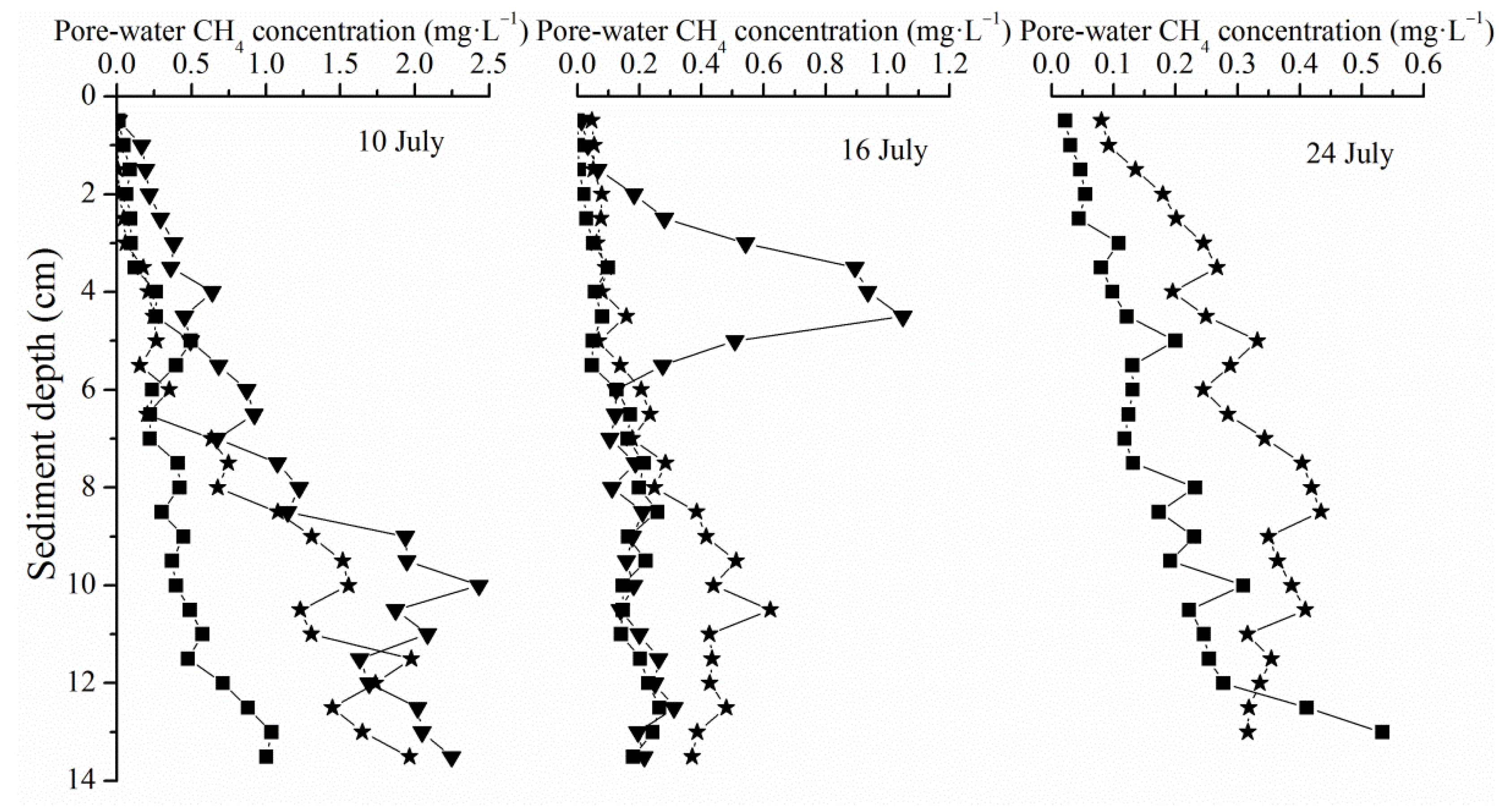
2.3. Pore-Water CH₄ Concentration

On 10th, 16th and 24th July, surface 15-cm sediment cores were collected using the 24 cm long and 3.4 cm diameter polymethyl methacrylate (PMMA) tubes near the collar base when the one day’s gas sampling was finished. The tubes were firstly inserted downward into the sediments. Then the tubes holding sediments were dug out and screwed immediately with the matched lids. Having been sealed, the sediment cores were immediately carried back to the laboratory for pore-water CH₄ concentration measurement. In the laboratory, sufficient distilled water was aerated by aeration pump for two hours to drive out the dissolved CH₄ in water and 60 mL aerated distilled water was injected into the PMMA pipes which had been rinsed twice with distilled water. The sediment cores were sectioned serially at 0.5 cm intervals and the sectioned slice was put into PMMA pipes held aerated distilled water quickly. Then, the pipes were covered with the caps which were lined with a silicone insole immediately. With all the preparation done, the PMMA pipes were placed on an automatic roller to shake up for 10 min to make the sediment dissolve in the aerated distilled water completely. Having been balanced in the ambient temperature in the laboratory for at least half an hour, a 10-mL gas sample at the upper space of the pipe was extracted with 20-mL syringes, whose top was fixed with a clinical three-way valve. CH₄ concentration of the gas samples were also measured by Agilent 7890A GC with its configurations as detailed above. The final pore-water concentration of CH₄ is calculated by the following equation:

$$C=\frac{\left[\left(C_{AIR}-C_{BLANK}\right)\times V_{AIR}+\left(C_{AIR}-C_{BLANK}\right)\times \mathsf{\alpha }\times V_{WATER}\right]}{V_{POREWATER}}$$

(1)

C was the pore-water CH₄ concentration (mg·L⁻¹); C_AIR was the CH₄ concentration in the upper pipe gas (mg·L⁻¹); C_BLANK was the CH₄ concentration of aerated distilled water without addition of a sample in the upper pipe gas (mg·L⁻¹); V_AIR was the volume of the upper gas of the pipe (L); α was the Busen coefficient; V_WATER represents the volume of aerated distilled water injected into the pipe (L); V_POREWATER was the corresponding volume of pore water in different depth of sample (L).

2.4. Environmental Parameters Measurement

Both air temperature and sediment’s ground temperature (GT) at different depths (5 cm, 10 cm and 15 cm) were recorded during the gas sampling. Light intensity was measured using a TES-1332 photometer. The mass balance method was used to measure sediment water content. The fresh sediment was weighed immediately after the sample was carried back to the laboratory and the dry weight was measured when the sediment was dried to a constant weight in 45 °C. For the lack of specific field records of tide elevation, the tide table of Hengsha station (31.293° N, 121.848° E), which was located near our study site (31.502° N, 121.984° E), was chosen as a tide height and inundation reference. We also compared the important climatic variables, including air temperature, precipitation, isolation duration, solar radiation and air pressure in July between the mean value of the last thirty years from 1991 to 2020 and the year 2011 to judge whether the sampling period was a normal year. The historical meteorological data were from the China Meteorological Administration (see the Supplementary Materials).

2.5. Data Processing

CH₄ fluxes were calculated by averaging the triple samples at each sampling time. The correlation relationship between the sediment–air interface flux and temperature were analyzed using SPSS 19.0 for windows. Besides, SPSS 19.0 was also used to test the significance of CH₄ flux variation during the 15-day tidal cycles. The results of the statistics were recognized as significant if p-values were lower than 0.05 or 0.01.

3. Results

3.1. Variation of Environmental Factors

Light intensity depends on cloud cover and other factors, thus solar radiation during the research period was variable. The strongest daily average light intensity appeared on the 16th and 19th July. Air temperature was significantly correlated with the light intensity, indicating that variation of air temperature was caused primarily by the change of light intensity (

Table 1. Correlation relationship between the CH₄ fluxes and environmental variables.

	Light Intensity	Air Temperature	5 cm GT	10 cm GT	15 cm GT	CH4 Fluxes
Light intensity	1
Air temperature	0.621 **	1
5 cm GT	0.544 **	0.976 **	1
10 cm GT	0.477 **	0.969 **	0.989 **	1
15 cm GT	0.504 **	0.973 **	0.985 **	0.974 **	1
CH4 flux	0.024	0.412 **	0.394 **	0.443 **	0.367 **	1

** represents p < 0.01.

). The highest daily average air temperature appeared on 19 July and the lowest appeared on 13 July. As a whole, air temperature was liable to be influenced by the solar radiation and other climatic variables and fluctuated during the research period. The ground temperature in different depths showed a relatively stable value due to the thermal insulation of sediment, which helped to prevent the underground sediment from being affected by the solar radiation too much (Figure 2). Besides, by the comparison of important climatic variables in July 2011 against the contemporaneous historical data of the last thirty years, it was found that the temperature was significantly higher than the mean value. The rest of the climatic variables such as precipitation, isolation duration, solar radiation and air pressure did not show any apparent differences between July 2011 and the historic average.

3.2. CH₄ Fluxes from the Neap to Spring Tide

During the 15-day observation, CH₄ emissions showed a general rising tendency (Figure 3). At the beginning of flux measurement on the 10th and the 13th July, CH₄ fluxes stayed at quite a low level and both of the two day average fluxes were only 0.68 mgCH₄·m⁻²·h⁻¹. The CH₄ emissions, especially in dark chambers on 16th July, apparently increased compared with the previous emissions (daily average flux on 16 July was 1.40 mgCH₄·m⁻²·h⁻¹). Influenced by the further elevated tide levels on 19th July, the salt marsh sediment together with the Scirpus mariqueter was submerged by the tide water during the whole day. The daily average CH₄ flux on 19th July decreased to 1.24 mg·m⁻²·h⁻¹, probably because the stoma of Scirpus mariqueter, which was the main escaping approach of plants, transported CH₄ sealed by the tide water. In the following two days’ observations, CH₄ flux exhibited a more significant increase compared with the previous fluxes (p < 0.05) and the daily average CH₄ fluxes reached 2.04 mgCH₄·m⁻²·h⁻¹ and 4.22 mgCH₄·m⁻²·h⁻¹ separately on the 22^nd and the 24th July. When compared with averaged CH₄ fluxes in light chambers, CH₄ fluxes were higher in dark chambers most of the time.

3.3. Pore-Water CH₄ Concentrations

The pore-water CH₄ concentration of the parallel samples presented apparent heterogeneity and the data were presented separately for the triplicate samples. Inconsistent with CH₄ flux variation, sediment pore-water CH₄ concentrations exhibited a roughly decreasing tendency during the 15-day tidal cycles. The highest CH₄ concentration profile appeared on 10th July and lower pore-water CH₄ concentrations appeared on 16th and 24th July. Vertically, the sediment pore-water CH₄ concentrations showed a significant increasing tendency with the sediment depth. During the three measurements within the depth of 15 cm, the highest pore-water CH₄ concentrations were 2.5 mg·L⁻¹, 1.2 mg·L⁻¹ and 0.6 mg·L⁻¹ separately (Figure 4).

3.4. Tide Variations during the Period of Flux Measurement

The first flux measurement on 10 July was carried out during the neap tide period with the highest tide level of 340 cm at 7:07 pm, which cannot submerge the salt marsh (

Table 2. The highest and lowest tide height during the 15-day tidal cycles.

Date	Time	Tide Height (cm)	Time	Tide Height (cm)
10 July	01:17	144	06:06	303
	13:21	115	19:07	340
13 July	05:36	110	10:15	298
	17:02	105	23:05	405
16 July	00:25	426	08:05	96
	12:33	356	19:29	102
19 July	01:29	416	09:27	110
	13:51	365	20:59	119
22 July	03:06	361	10:07	107
	15:45	339	22:24	147
24 July	04:37	284	11:23	133
	17:43	309

). That is, before gas sampling on 10 July, salt marsh sediment was exposed in the air for quite a long time. The tide level rose in the following days and the highest tide reached 402 cm on 13th July. Although the salt marsh sediment was not submerged by tide water in daytime, the nighttime tide could rise to a height high enough to submerge the salt marsh. Two days later, with arrival of the spring tide on 16th July, the tide height reached its the highest elevation (426 cm) of July. However, the appearance of the spring tide did not mean the longest inundation time for salt marsh sediment because the height of the spring low tide was also the lowest of the month. When the spring tide appeared, movement of tide water was very quick no matter in the rising movement or in the ebbing movement and the tide water could reach the area of higher altitude, including both salt marsh and high tidal flat covered by Phragmites australis. During the study period, the longest inundation condition of the salt marsh appeared on 19th July although the spring tide had already passed. The reduction of the height difference between the high tide and the low tide slowed down the speed of the tide movement and thus it prolonged the inundation time. Tide water failed to reach the salt marsh on 22^nd and 24th July in daytime because of the decreasing tide height, which finally caused the inundation time decrease sharply. The inundation time sharply decreased on these two days. Water contents of the surface 1 cm sediments were separately 44%, 68% and 56% on 10, 16 and 24 July, corresponding well with the sediment inundation condition.

4. Discussion

4.1. Variations of CH₄ Emissions during the Tide Cycle

Estuarine salt marshes acted as the strong sources of atmospheric CH₄ in our study, which was also indicated by numerous previous studies [28,29,30,31]. The magnitudes of CH₄ emission fluxes in light and dark conditions from salt marshes in our study were separately in the range of 0.60 mgCH₄·m⁻²·h⁻¹ to 2.60 mgCH₄·m⁻²·h⁻¹ and 0.56 mgCH₄·m⁻²·h⁻¹ to 5.85 mgCH₄·m⁻²·h⁻¹ during summer time. It suggested that even in a very short period (15-day tidal cycles last half month), CH₄ fluxes varied significantly. The strongest CH₄ emission on 24th July (4.22 mgCH₄·m⁻²·h⁻¹) was six times that of the weakest emission (0.68 mgCH₄·m⁻²·h⁻¹) on 10th July. The amplitude of CH₄ emission variation during the 15-day research was also nearly six times bigger than that between March and June (the minimum flux was 0.074 mgCH₄·m⁻²·h⁻¹ in March during the year according to our field measurement). Many studies were inclined to focus on the long-term variation of CH₄ emission including the monthly, seasonal and even yearly scale. During these long-term observations, CH₄ flux of one day or even a very limited period of a certain day was usually extrapolated to be the average flux for this period (monthly, seasonal or interannual) [19,24,32,33]. In our study, CH₄ fluxes during the 15-day observation presented a gradual increase before the spring tide and a steep increase after the spring tide. There existed a significant difference of daily average CH₄ flux between 19th July and 22^nd July (p < 0.05), while there were no significant differences for other days (p > 0.05). If daily average CH₄ fluxes of different dates, even during the short term, were selected to represent the monthly or even seasonal CH₄ emission, large differences would occur. For instance, if we separately took the daily fluxes on 10th and 24th July as the representative flux for the entirety of August, the results would exhibit a septuple difference. Based on the significant differences of the CH₄ fluxes in two consecutive observations within no more than four days, the common chamber-chromatograph method of averaging discontinuous measurements carried out at long time intervals to obtain seasonal or even annual fluxes was proved to have a lack of accuracy. In Allen’s research, CH₄ flux in costal mangrove wetland sediment increased from 0.25 mgCH₄·m⁻²·h⁻¹ to 1.57 mgCH₄·m⁻²·h⁻¹ from winter to summer and the peak value in summer was about seven times bigger than the lowest value in winter with this multiple, which is very close to that of our research in 15 days [34]. Miao has completed relatively frequent research into CH₄ emissions in wetland at one week intervals and a smooth change curve of CH₄ flux was obtained, which indicated that CH₄ flux changed unevenly with time and higher observation resolution resulted in a more accurate average emission flux [35]. Besides, Pearson also measured CH₄ flux at a 2–4 week interval in summertime and at monthly to bimonthly intervals in winter to obtain more exact CH₄ fluxes [36]. High time resolution of CH₄ fluxes obtained by the eddy correlation system showed that short-term variability was more evident in summer, along with the pronounced temperature changes being more pronounce and it diminished in colder weather [37]. Except for the sharp rise of temperature in summer, which could cause a corresponding increase of CH₄ emissions, the growth of wetland plants under high temperatures improved the uncertainty of CH₄ biochemical processes [38]. CH₄ emissions caused by plant growing could account for more than 90% of the total annual flux [39].

The Yangtze estuary, located in the East Asia with a subtropical monsoon climate, has four distinctive seasons. CH₄ fluxes increased from spring with temperature increase and peaked in summer [27]. However, the CH₄ emission increased slowly in spring and greatly in summer. To obtain more accurate average CH₄ flux, it is necessary to properly increase the observation times and days especially during the changeable periods of CH₄ emission. Otherwise, the extrapolated annual CH₄ emission would result in under- or over-estimation of CH₄ flux, depending on the day it was measured.

4.2. Main Environmental Factors Driving the Tidal Variation of CH₄ Emission

Many previous studies have investigated the CH₄ fluxes and the key environmental control factors in various types of wetlands in a relatively long time scale such as the seasonal or annual variations [34,40,41,42,43]. The net CH₄ emission fluxes were the result of the combined actions of CH₄ production, consumption and transportation [44]. Therefore, theoretically, any environmental factor that could influence the above three processes could exert an influence on the final CH₄ emission fluxes. In practice, seasonal variations in the CH₄ emissions could be explained by the combined effect of the changes in soil temperature and the condition of the water in most cases. Several studies specifically indicated that CH₄ production had a strong correlation with Q₁₀ values varied in a wide range [45,46]. The long-term effect of temperature on CH₄ emission is attributed to its direct influence on the activity of methanogenic bacteria in the anoxic environment [47]. However, the mechanism of temperature control over the short-term CH₄ emission whose variation amplitude may be not much smaller than the annual variation amplitude was seldom studied. Our study results showed that CH₄ emissions in the semi-diurnal tidal estuary increased all along from one neap-tide day to another neap-tide day with the high-tide appearing in the mid-term. The highest CH₄ flux did not appear on the day with the highest air temperature. By Pearson correlation analysis, CH₄ fluxes were positively correlated with temperature, including both air temperature and ground temperature in different depths (5 cm GT, 10 cm GT and 15 cm GT) (p < 0.01). The strongest correlation relationship existed between 10 cm and CH₄ flux (R = 0.443, p < 0.01) (Table 1). However, the correlation coefficient was significantly less than that of the previous studies on long-term seasonal variations of CH₄ emissions [24,34]. This indicated that the degree of temperature explanation for CH₄ emissions during the short term of semi-monthly tide cycles decreased apparently compared with that in the long time scale researches.

Sediment pore-water CH₄ concentration was always linked with diffusive CH₄ flux according to Fick’s law, which indicates that molecule diffusion occurred towards the concentration decrease direction [48]. The pore-water CH₄ in surface sediment concentration here was also taken to help explain the dominant CH₄ emission pattern of vegetated salt marshes. The static pore-water CH₄ concentration was the result of the dynamic procedure of CH₄ production and consumption [23]. When the production rate exceeds the consumption rate, CH₄ concentration increased, otherwise, it decreased. The pore-water CH₄ concentration in the surface layer of the sediment directly determines the diffusion flux [48]. The calculated diffusion CH₄ flux by Fick’s law was less than 0.42 mgCH₄·m⁻²·h⁻¹ when the near-surface pore-water CH₄ concentration varied from 0 to 8 mg·L⁻¹ [49]. Previous studies also indicated that bubbles could not form until pore-water CH₄ concentrations exceeded 7.4 mg·L⁻¹ ~ 8.0 mg·L⁻¹ [16]. In our research, within 15 cm from the surface, the pore-water CH₄ concentration was very low (the highest observed pore-water CH₄ concentration was 2.5 mg·L⁻¹), which led to a weak diffusion flux, not to mention the bubble ebullition, and thus it could be roughly speculated that the plant transport functioned as the primary means of CH₄ emission. Besides, along with the tidal variation, the pore-water CH₄ concentration did not exhibit an apparent variation. Pore-water CH₄ concentration also showed no consistent change with temperature increase, which was probably because of the dual effects of the increasing temperature on both the production rate and the consumption rate of CH₄ [50]. In consideration of the numerous studies on CH₄ transport by wetland plants, only the constantly growing biomass during this period, which usually continued to August, could better correspond with the ever increasing CH₄ fluxes and explain the decreased correlation coefficient of temperature and short-term CH₄ fluxes compared with the long-term variation.

Although tide is an important physical process that influences biogeochemical processes in coastal wetlands, there have been few attempts to determine CH₄ emission variation through the entire tidal cycle including both the neap and the spring tide period [51]. Tidal movement could influence CH₄ emissions directly in many ways, including changing the sediment hydrology condition, newly sedimentation and salinity etc. Tidal movement could also exert a indirect influence on CH₄ emission through the plant transportation. If the tide level is high enough to submerge the wetland plant, it would obviously weaken the CH₄ transportation, thus resulting in greatly reduced CH₄ emissions. In our research, the minimum CH₄ flux appeared at 12:00 and 13:30 on 19th July when the tide water submerged the salt mash together with the Scirpus mariqueter. The CH₄ emissions through the leaf stomata was greatly reduced by the tide water. However, CH₄ fluxes showed no correlation with tide levels (R = −0.014, p = 0.979), which were related to the inundation time and frequency. It was reported in a previous study that inundation time greatly influenced the production and emission of CH₄ by creating a more anaerobic condition [52,53]. In our studied salt marshes, the inundation time increased day by day before 19th July and decreased after 19th July when the spring tide period passed. During the whole period, CH₄ fluxes increased all along without being influenced by tidal activity and the inundation time. It is probably because the differences of inundation conditions caused by the tide movement are not big enough to apparently influence the underground CH₄ productions.

In synthesizing all the potential environmental drivers for the tidal variations of CH₄, both air and ground temperature and wetland plant transport for CH₄ by its aerenchyma were the most important factors influencing the short-term CH₄ emissions (Figure 5). Different to the seasonal variations of CH₄ emissions, the short-term effect of temperature on CH₄ emissions was confounded by plant growth to some degree. It was found by the previous study that the biomass of the sedge plant in the salt marsh of the Yangtze estuary could increase from 364.1 to 692.6 g·dm·m⁻² only a month later from July to August, which just covered this research period [27]. The dramatically increased CH₄ just appeared at the vigorous growing stage. If the study scale was extended to one year, the temperature would exhibit higher matching with plant growing. On the contrary, the plant growing and temperature increase could separate ways in July when the air temperature has already reached its maximum of the year, while the plant was still vigorously growing. The strengthened capacity of CH₄ transportation, more than any other factor, better explained the depressed correlation relationship between short-term CH₄ emissions and temperature. Moreover, in consideration of the significant differences of CH₄ fluxes in the short-term during the plant growing period, high-frequency observations of CH₄ emissions are necessary, especially during the exuberant growth period, in order to obtain accurate gas fluxes. Otherwise, the obtained fluxes would be greatly under- or over-estimated.

5. Conclusions

This study suggested that CH₄ emissions varied significantly during the tide cycles. The sediment–air CH₄ fluxes increased from 0.68 to 4.22 mgCH₄·m⁻²·h⁻¹ during the 15 days’ tidal cycle from 10 July to 24 July. This demonstrated that July is a critical developmental period for CH₄ emissions in the Yangtze estuary intertidal zones. By correlation analysis, both tide levels and solar radiation did not correlate with CH₄ fluxes. The fluxes were also not influenced by the inundation time. Both air and ground temperature were proved to be the key environmental factors controlling CH₄ fluxes during the tide cycles. However, the correlation coefficient between the temperature and CH₄ fluxes in this short-term study decreased compared with that in the long-term, annual scale, indicating that there are some other important environmental factor(s) which greatly influenced the short-term CH₄ emission variations. It was found that the dramatically increased CH₄ just appeared at the vigorous growing stage. Therefore, different to the seasonal variations of CH₄ emissions, the short-term effect of temperature on CH₄ emissions could be possibly confounded by plant growth to some degree. The pore-water CH₄ concentrations measured every 5 days during the research period were not correlated with the ever-increasing CH₄ fluxes, indicating that CH₄ fluxes were also not mainly determined by the underground methanogenic processes. In terms of emission processes, generally low pore-water CH₄ concentrations eliminate the possibility of CH₄ gas bubble emissions. This further underscores the importance of plant transportation for CH₄ emissions in the vegetated tidal wetland, no matter in the long annual research (investigated in our previous research) or in the short tide cycles. Except for Scirpus mariqueter, there are two other kinds of gramineae plants (Phragmites and Spartina alterniflora) whose aerenchyma are more developed, in the Yangtze Estuary intertidal zone. In order to comprehensively understand the effects of invasive vegetation on CH₄ emissions in this area, further investigations need to be carried out in the future.

References

1. Singh, J.S.; Gupta, V.K. Degraded Land Restoration in Reinstating CH4 Sink. Front. Microbiol. 2016, 7, 923. [Google Scholar] [CrossRef] [PubMed]
2. IPCC. Climate Change 2013: The Physical Science Basis; IPCC: Geneva, Switzerland, 2013. [Google Scholar]
3. Shindell, D.T.; Faluvegi, G.; Koch, D.M.; Schmidt, G.A.; Unger, N.; Bauer, S.E. Improved Attribution of Climate Forcing to Emissions. Science 2009, 326, 716–718. [Google Scholar] [CrossRef] [PubMed] [Green Version]
4. Pickett-Heaps, C.A.; Jacob, D.J.; Wecht, K.J.; Kort, E.A.; Wofsy, S.C.; Diskin, G.S.; Worthy, D.E.J.; Kaplan, J.O.; Bey, I.; Drevet, J. Magnitude and seasonality of wetland methane emissions from the Hudson Bay Lowlands (Canada). Atmos. Chem. Phys. 2011, 11, 37733779. [Google Scholar] [CrossRef] [Green Version]
5. Vizza, C.; West, W.E.; Jones, S.E.; Hart, J.A.; Lamberti, G.A. Regulators of coastal wetland methane production and responses to simulated global change. Biogeosciences 2017, 14, 431–446. [Google Scholar] [CrossRef] [Green Version]
6. Nahlik, A.M.; Mitsch, W.J. Methane emissions from tropical freshwater wetlands located in different climatic zones of Costa Rica. Glob. Chang. Biol. 2011, 17, 1321–1334. [Google Scholar] [CrossRef]
7. Zhang, L.; Wang, M.H.; Hu, J.; Ho, Y.S. A review of published wetland research, 1991–2008: Ecological engineering and ecosystem restoration. Ecol. Eng. 2010, 36, 973–980. [Google Scholar] [CrossRef]
8. Bhullar, G.S.; Edwards, P.J.; Venterink, H.O. Influence of Different Plant Species on Methane Emissions from Soil in a Restored Swiss Wetland. PLoS ONE 2014, 9, e89588. [Google Scholar] [CrossRef] [Green Version]
9. Xie, X.; Zhang, M.Q.; Zhao, B.; Guo, H.Q. Dependence of coastal wetland ecosystem respiration on temperature and tides: A temporal perspective. Biogeosciences 2014, 11, 539–545. [Google Scholar] [CrossRef] [Green Version]
10. Abdul-Aziz, O.I.; Ishtiaq, K.S.; Tang, J.W.; Moseman-Valtierra, S.; Kroeger, K.D.; Gonneea, M.E.; Mora, J.; Morkeski, K. Environmental Controls, Emergent Scaling, and Predictions of Greenhouse Gas (GHG) Fluxes in Coastal Salt Marshes. J. Geophys. Res. Biogeosci. 2018, 123, 2234–2256. [Google Scholar] [CrossRef]
11. Poffenbarger, H.J.; Needelman, B.A.; Megonigal, J.P. Salinity Influence on Methane Emissions from Tidal Marshes. Wetlands 2011, 31, 831–842. [Google Scholar] [CrossRef]
12. Jeffrey, L.C.; Maher, D.T.; Johnston, S.G.; Kelaher, B.P.; Steven, A.; Tait, D.R. Wetland methane emissions dominated by plant-mediated fluxes: Contrasting emissions pathways and seasons within a shallow freshwater subtropical wetland. Limnol. Oceanogr. 2019, 64, 1895–1912. [Google Scholar] [CrossRef]
13. Mueller, P.; Mozdzer, T.J.; Langley, J.A.; Aoki, L.R.; Noyce, G.L.; Megonigal, J.P. Plant species determine tidal wetland methane response to sea level rise. Nat. Commun. 2020, 11. [Google Scholar] [CrossRef]
14. Al-Haj, A.N.; Fulweiler, R.W. A synthesis of methane emissions from shallow vegetated coastal ecosystems. Glob. Chang. Biol. 2020, 26, 2988–3005. [Google Scholar] [CrossRef]
15. Sturm, K.; Werner, U.; Grinham, A.; Yuan, Z.G. Tidal variability in methane and nitrous oxide emissions along a subtropical estuarine gradient. Estuar. Coast. Shelf Sci. 2017, 192, 159–169. [Google Scholar] [CrossRef]
16. Baird, A.J.; Beckwith, C.W.; Waldron, S.; Waddington, J.M. Ebullition of methane-containing gas bubbles from near-surface Sphagnum peat. Geophys. Res. Lett. 2004, 31. [Google Scholar] [CrossRef]
17. Kao-Kniffin, J.; Freyre, D.S.; Balser, T.C. Methane dynamics across wetland plant species. Aquat. Bot. 2010, 93, 107–113. [Google Scholar] [CrossRef]
18. Askaer, L.; Elberling, B.; Friborg, T.; Jorgensen, C.J.; Hansen, B.U. Plant-mediated CH4 transport and C gas dynamics quantified in-situ in a Phalaris arundinacea—Dominant wetland. Plant Soil 2011, 343, 287–301. [Google Scholar] [CrossRef]
19. Smemo, K.A.; Yavitt, J.B. Anaerobic oxidation of methane: An underappreciated aspect of methane cycling in peatland ecosystems? Biogeosciences 2011, 8, 779–793. [Google Scholar] [CrossRef] [Green Version]
20. Fritz, C.; Pancotto, V.A.; Elzenga, J.T.M.; Visser, E.J.W.; Grootjans, A.P.; Pol, A.; Iturraspe, R.; Roelofs, J.G.M.; Smolders, A.J.P. Zero methane emission bogs: Extreme rhizosphere oxygenation by cushion plants in Patagonia. New Phytol. 2011, 190, 398–408. [Google Scholar] [CrossRef]
21. Segers, R. Methane production and methane consumption: A review of processes underlying wetland methane fluxes. Biogeochemistry 1998, 41, 23–51. [Google Scholar] [CrossRef]
22. Tang, J.; Zhuang, Q.; Shannon, R.D.; White, J.R. Quantifying wetland methane emissions with process-based models of different complexities. Biogeosciences 2010, 7, 3817–3837. [Google Scholar] [CrossRef] [Green Version]
23. Li, Y.J.; Wang, D.Q.; Chen, Z.L.; Hu, H. Comprehensive effects of a sedge plant on CH4 and N2O emissions in an estuarine marsh. Estuar. Coast. Shelf Sci. 2018, 204, 202–211. [Google Scholar] [CrossRef]
24. Wang, D.Q.; Chen, Z.L.; Xu, S.Y. Methane emission from Yangtze estuarine wetland, China. J. Geophys. Res. Biogeosci. 2009, 114. [Google Scholar] [CrossRef] [Green Version]
25. Yuan, Y.Q.; Li, X.Z.; Jiang, J.Y.; Xue, L.M.; Craft, C.B. Distribution of organic carbon storage in different salt-marsh plant communities: A case study at the Yangtze Estuary. Estuar. Coast. Shelf Sci. 2020, 243. [Google Scholar] [CrossRef]
26. Sun, S.C.; Cai, Y.L.; An, S.Q. Differences in morphology and biomass allocation of Scirpus mariqueter between creekside and inland communities in the Changjiang estuary, China. Wetlands 2002, 22, 786–793. [Google Scholar] [CrossRef]
27. Li, Y.J.; Wang, D.Q.; Chen, Z.L.; Jin, H.Y.; Hu, H.; Chen, J.F.; Yang, Z. Role of Scirpus mariqueter on Methane Emission from an Intertidal Saltmarsh of Yangtze Estuary. Sustainability 2018, 10, 1139. [Google Scholar] [CrossRef] [Green Version]
28. Li, Y.; Zhan, L.; Chen, L.; Zhang, J.; Wu, M.; Liu, J. Spatial and temporal patterns of methane and its influencing factors in the Jiulong River estuary, southeastern China. J. Mar. Chem. 2020, 228, 103909. [Google Scholar] [CrossRef]
29. Livesley, S.J.; Andrusiak, S.M. Temperate mangrove and salt marsh sediments are a small methane and nitrous oxide source but important carbon store. Estuar. Coast. Shelf Sci. 2012, 97, 19–27. [Google Scholar] [CrossRef]
30. Rosentreter, J.A.; Maher, D.T.; Erler, D.V.; Murray, R.; Eyre, B.D. Factors controlling seasonal CO2 and CH4 emissions in three tropical mangrove-dominated estuaries in Australia. Estuar. Coast. Shelf Sci. 2018, 215, 69–82. [Google Scholar] [CrossRef]
31. Kim, J.; Lee, J.; Yun, J.; Yang, Y.R.; Ding, W.X.; Yuan, J.J.; Kang, H. Mechanisms of enhanced methane emission due to introduction of Spartina anglica and Phragmites australis in a temperate tidal salt marsh. Ecol. Eng. 2020, 153, 105905. [Google Scholar] [CrossRef]
32. Cheng, X.L.; Luo, Y.Q.; Xu, Q.; Lin, G.H.; Zhang, Q.F.; Chen, J.K.; Li, B. Seasonal variation in CH4 emission and its C-13-isotopic signature from Spartina alterniflora and Scirpus mariqueter soils in an estuarine wetland. Plant Soil 2010, 327, 85–94. [Google Scholar] [CrossRef] [Green Version]
33. Hu, M.J.; Ren, H.X.; Ren, P.; Li, J.B.; Wilson, B.J.; Tong, C. Response of gaseous carbon emissions to low-level salinity increase in tidal marsh ecosystem of the Min River estuary, southeastern China. J. Environ. Sci 2017, 52, 210–222. [Google Scholar] [CrossRef] [PubMed]
34. Allen, D.E.; Dalal, R.C.; Rennenberg, H.; Meyer, R.L.; Reeves, S.; Schmidt, S. Spatial and temporal variation of nitrous oxide and methane flux between subtropical mangrove sediments and the atmosphere. Soil Biol. Biochem. 2007, 39, 622–631. [Google Scholar] [CrossRef]
35. Miao, Y.; Song, C.; Sun, L.; Wang, X.; Meng, H.; Mao, R. Growing season methane emission from a boreal peatland in the continuous permafrost zone of Northeast China: Effects of active layer depth and vegetation. Biogeosciences 2012, 9, 4455–4464. [Google Scholar] [CrossRef] [Green Version]
36. Pearson, M.; Saarinen, M.; Minkkinen, K.; Silvan, N.; Laine, J. Short-term impacts of soil preparation on greenhouse gas fluxes: A case study in nutrient-poor, clearcut peatland forest. For. Ecol. Manag. 2012, 283, 10–26. [Google Scholar] [CrossRef]
37. Jackowicz-Korczynski, M.; Christensen, T.R.; Backstrand, K.; Crill, P.; Friborg, T.; Mastepanov, M.; Strom, L. Annual cycle of methane emission from a subarctic peatland. J. Geophys. Res. Biogeosci. 2010, 115. [Google Scholar] [CrossRef]
38. Strom, L.; Mastepanov, M.; Christensen, T.R. Species-specific effects of vascular plants on carbon turnover and methane emissions from wetlands. Biogeochemistry 2005, 75, 65–82. [Google Scholar] [CrossRef]
39. Song, C.C.; Xu, X.F.; Tian, H.Q.; Wang, Y.Y. Ecosystem-atmosphere exchange of CH4 and N2O and ecosystem respiration in wetlands in the Sanjiang Plain, Northeastern China. Glob. Chang. Biol. 2009, 15, 692–705. [Google Scholar] [CrossRef]
40. Moore, T.R.; De Young, A.; Bubier, J.L.; Humphreys, E.R.; Lafleur, P.M.; Roulet, N.T. A Multi-Year Record of Methane Flux at the Mer Bleue Bog, Southern Canada. Ecosystems 2011, 14, 646–657. [Google Scholar] [CrossRef]
41. Sun, Z.G.; Jiang, H.H.; Wang, L.L.; Mou, X.J.; Sun, W.L. Seasonal and spatial variations of methane emissions from coastal marshes in the northern Yellow River estuary, China. Plant Soil 2013, 369, 317–333. [Google Scholar] [CrossRef] [Green Version]
42. Tong, C.; Huang, J.F.; Hu, Z.Q.; Jin, Y.F. Diurnal Variations of Carbon Dioxide, Methane, and Nitrous Oxide Vertical Fluxes in a Subtropical Estuarine Marsh on Neap and Spring Tide Days. Estuar. Coasts 2013, 36, 633–642. [Google Scholar] [CrossRef]
43. Wright, E.L.; Black, C.R.; Turner, B.L.; Sjogersten, S. Environmental controls of temporal and spatial variability in CO2 and CH4 fluxes in a neotropical peatland. Glob. Chang. Biol. 2013, 19, 3775–3789. [Google Scholar] [CrossRef] [PubMed]
44. Lai, D.Y.F. Methane Dynamics in Northern Peatlands: A Review. Pedosphere 2009, 19, 409–421. [Google Scholar] [CrossRef]
45. Dunfield, P.; Knowles, R.; Dumont, R.; Moore, T.R. Methane production and consumption in temperate and subarctic peat soils: Response to temperature and pH. Soil Biol. Biochem. 1993, 25, 321–326. [Google Scholar] [CrossRef]
46. Moosavi, S.C.; Crill, P.M. CH4 oxidation by tundra wetlands as measured by a selective inhibitor technique. J. Geophys. Res. Atmos. 1998, 103, 29093–29106. [Google Scholar] [CrossRef]
47. Heyer, J.; Berger, U. Methane emission from the coastal area in the southern Baltic Sea. Estuar. Coast. Shelf Sci. 2000, 51, 13–30. [Google Scholar] [CrossRef]
48. Elberling, B.; Askaer, L.; Jorgensen, C.J.; Joensen, H.P.; Kuhl, M.; Glud, R.N.; Lauritsen, F.R. Linking Soil O2, CO2, and CH4 Concentrations in a Wetland Soil: Implications for CO2 and CH4 Fluxes. Environ. Sci. Technol. 2011, 45, 3393–3399. [Google Scholar] [CrossRef] [PubMed]
49. Hornibrook, E.R.C.; Bowes, H.L.; Culbert, A.; Gallego-Sala, A.V. Methanotrophy potential versus methane supply by pore water diffusion in peatlands. Biogeosciences 2009, 6, 1490–1504. [Google Scholar] [CrossRef] [Green Version]
50. Boeckx, P.; VanCleemput, O. Methane oxidation in a neutral landfill cover soil: Influence of moisture content, temperature, and nitrogen-turnover. J. Environ. Qual. 1996, 25, 178–183. [Google Scholar] [CrossRef]
51. Tong, C.; Wang, W.Q.; Zeng, C.S.; Marrs, R. Methane (CH4) emission from a tidal marsh in the Min River estuary, southeast China. J. Environ. Sci. Health A 2010, 45, 506–516. [Google Scholar] [CrossRef]
52. Ding, W.X.; Zhang, Y.H.; Cai, Z.C. Impact of permanent inundation on methane emissions from a Spartina alterniflora coastal salt marsh. Atmos. Environ. 2010, 44, 3894–3900. [Google Scholar] [CrossRef]
53. Ma, A.N.; Lu, J.J.; Wang, T.H. Effects of Elevation and Vegetation on Methane Emissions from a Freshwater Estuarine Wetland. J. Coast. Res. 2012, 28, 1319–1329. [Google Scholar] [CrossRef]
Figure 1. Study site in the salt marshes of the Yangtze estuary covered by the Scirpus mariqueter.
Atmosphere 12 00245 g001
Figure 2. Variations of environmental factors during the research period.
Atmosphere 12 00245 g002
Figure 3. Variations of CH4 fluxes in both dark and light chamber during the 15-day tidal cycles.
Atmosphere 12 00245 g003
Figure 4. Sediment pore-water CH4 concentrations in different inundation conditions.
Atmosphere 12 00245 g004
Figure 5. Schematic diagram of the main controlling mechanisms of short-term CH4 emissions in the studied area.
Atmosphere 12 00245 g005