
2019–20 Australian Bushfires and Anomalies in Carbon Monoxide Surface and Column Measurements

 ,
,  ,
, .jpg) , ,
, ,
Abstract
:1. Introduction
- how anomalous were the black summer fires in the terms of the CO surface concentrations and column amounts at Wollongong?
- how well do enhancements in total column amounts of CO at Wollongong match the enhancements in surface in situ CO measurements? (Here, we use the word ‘enhancement’ to mean the amount that CO is increased above the defined background)
2. Methods
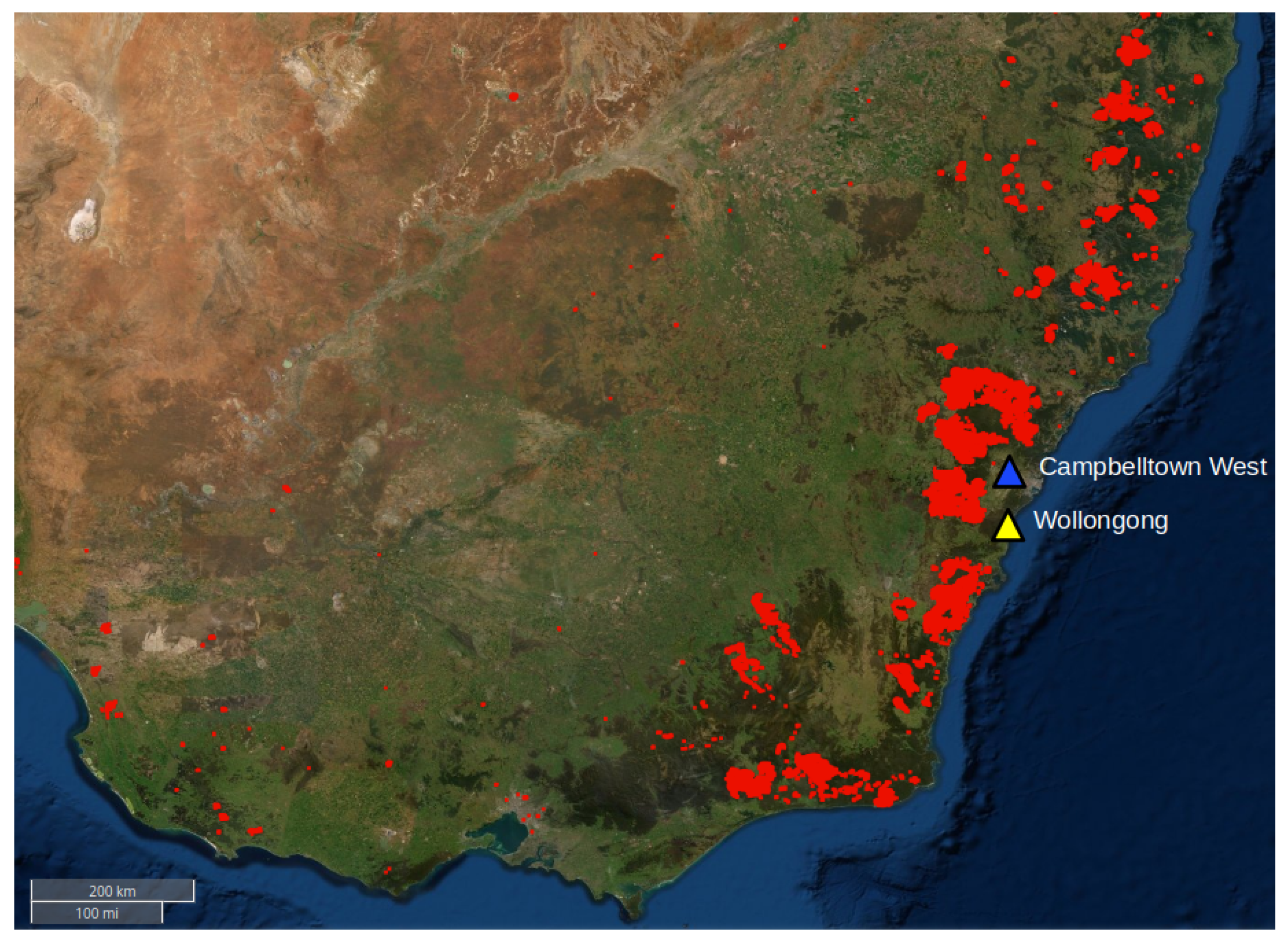
2.1. Site Description
2.2. In Situ FTIR
2.3. Total Carbon Column Observing Network (TCCON)
2.4. Network for the Detection of Atmospheric Composition Change (NDACC)
2.5. Air Quality Datasets
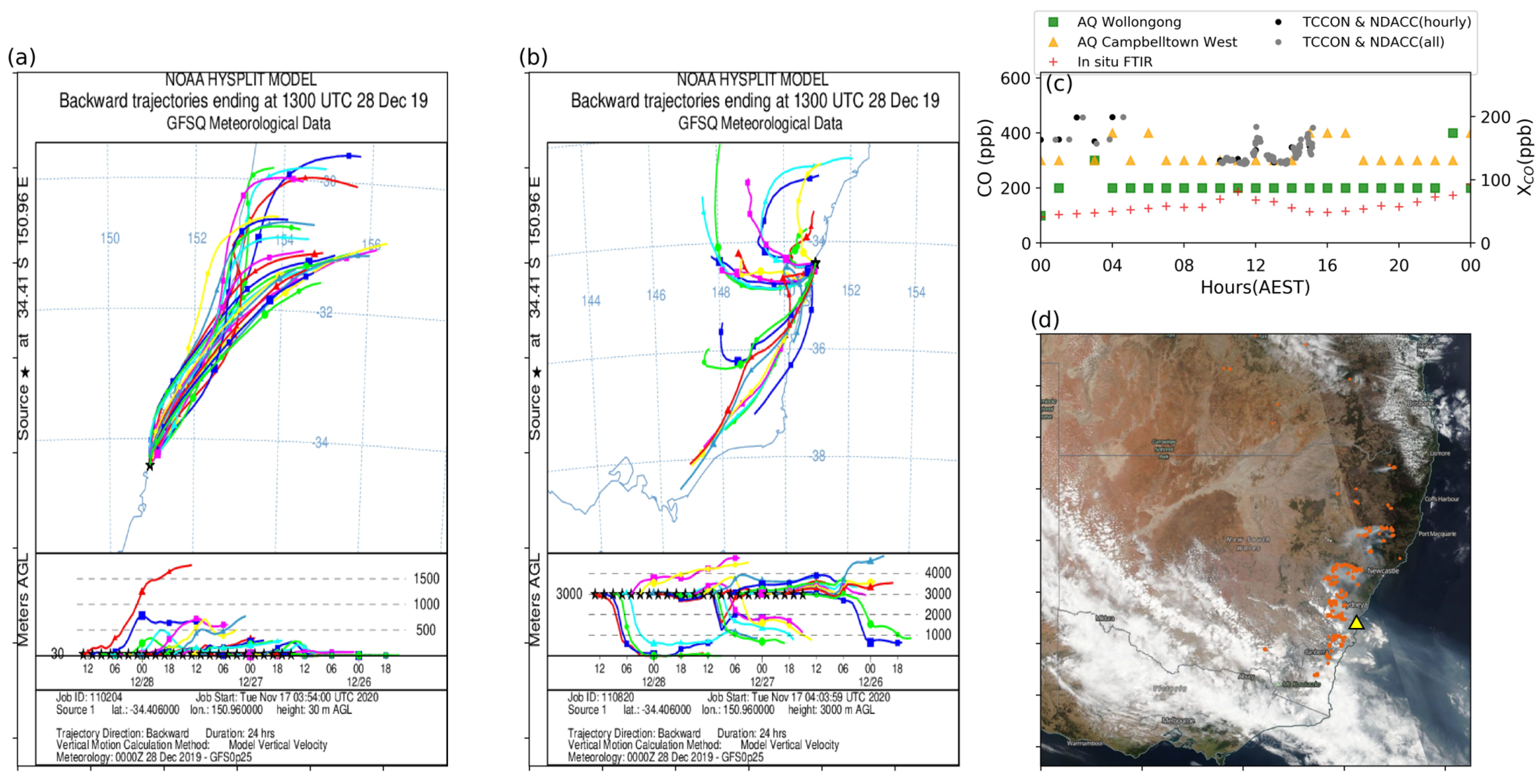
2.6. HYSPLIT Back Trajectories
3. Results
4. Discussion and Analysis of Anomalies
4.1. Wollongong X and Surface CO Anomalies
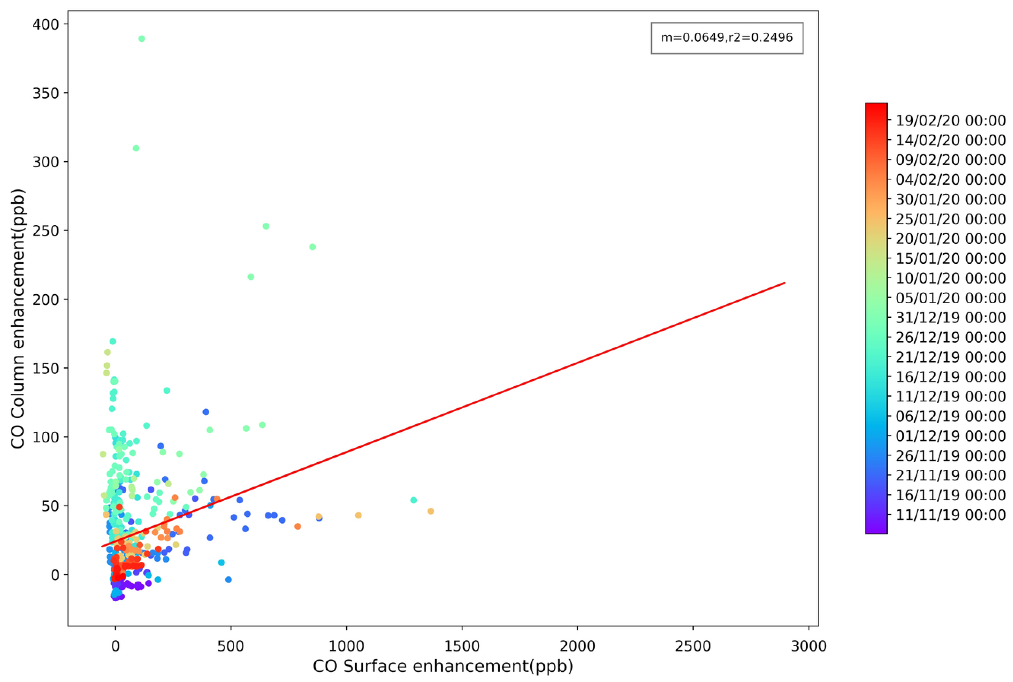
4.2. How Well Do Enhancements in Total Column Amounts of CO at Wollongong Match the Enhancements in Surface CO?
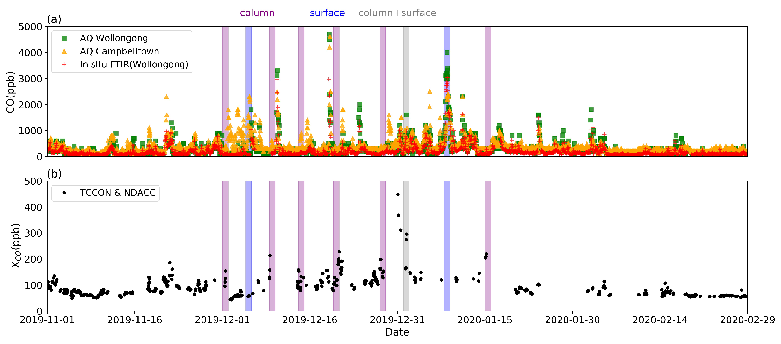
- CO enhancements in the column only
- CO enhancements in both column & surface in situ
- CO enhancements in the surface in situ only
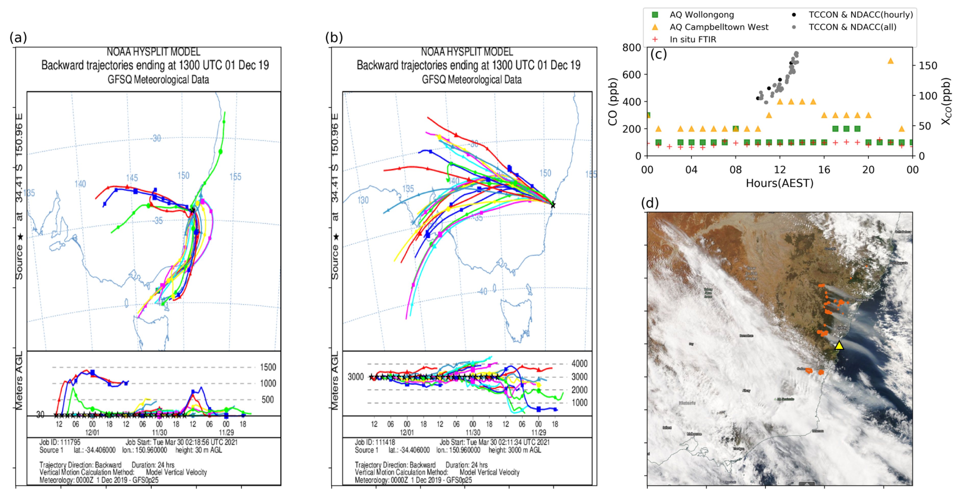
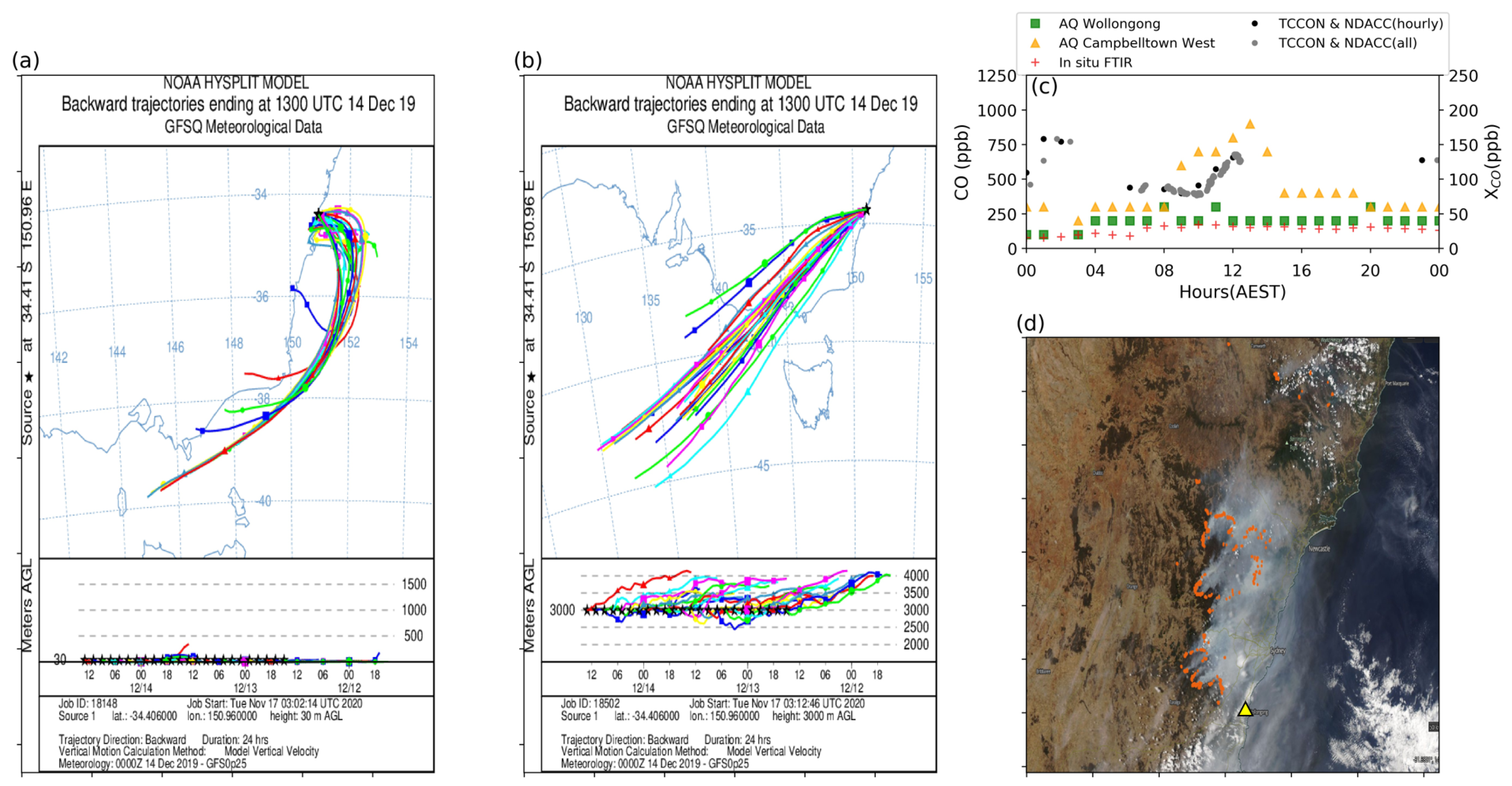
4.2.1. CO Enhancements in the Column Only
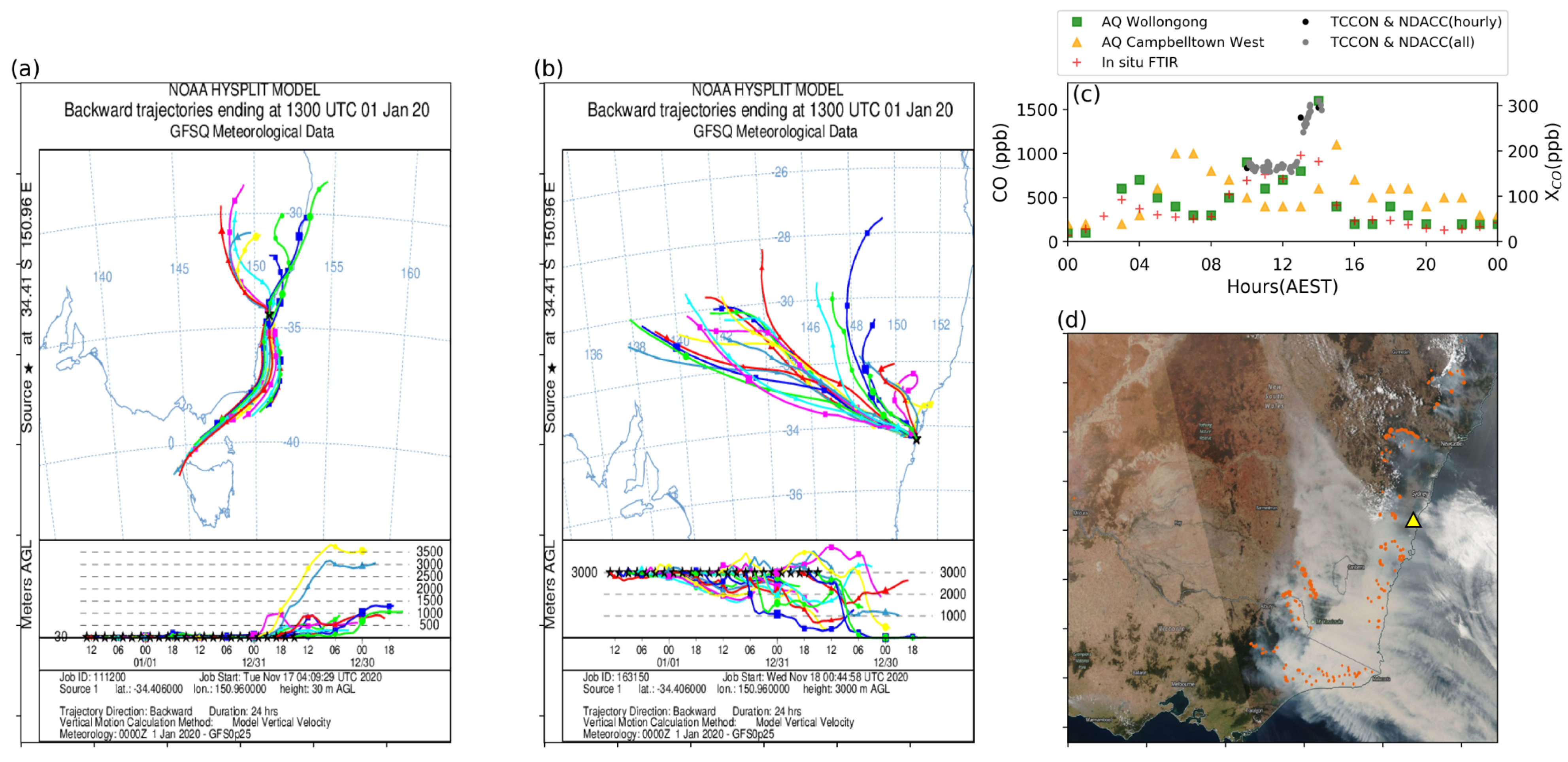
4.2.2. CO Enhancements in Both the Column & Surface In Situ
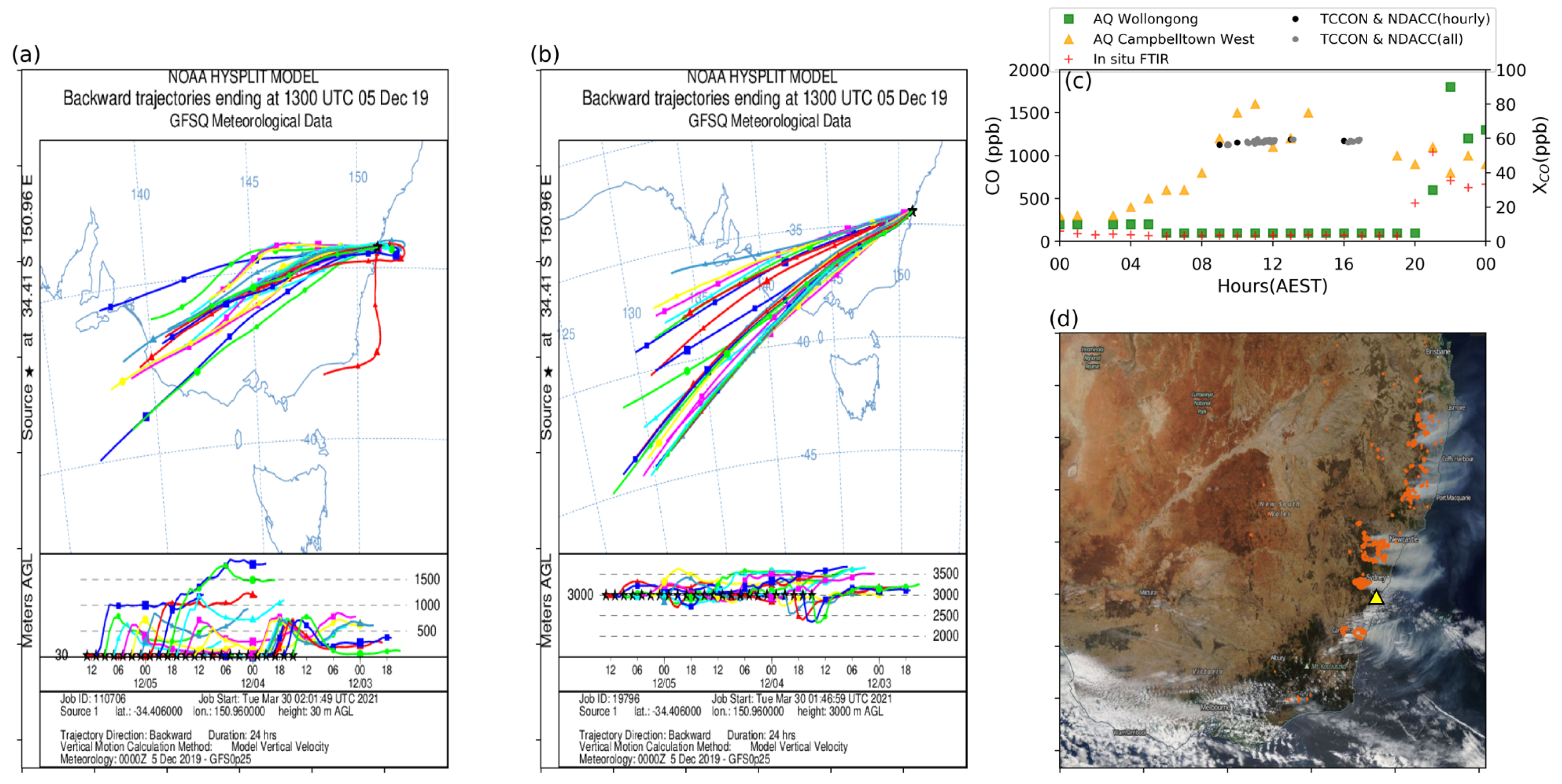
4.2.3. CO Enhancements in the Surface In Situ Only
5. Summary and Conclusions
Author Contributions
Funding
Institutional Review Board Statement
Informed Consent Statement
Data Availability Statement
Conflicts of Interest
Appendix A. Conversion of CO Total Column to XCO
- = Column averaged dry air mole fraction;
- = Vertical column of gas i;
- = Surface Pressure (mb);
- = Absorber weighted gravitational accleration;
- = Molecular mass of dry air, 28.964 g mol; and
- = Molecular mass of HO, 18.02 g mol.
Appendix B. CO Enhancements in the Column with Minor Enhancements at the Surface
Appendix C. Additional Plots
References
- Nolan, R.H.; de Dios, V.R.; Boer, M.M.; Caccamo, G.; Goulden, M.L.; Bradstock, R.A. Predicting dead fine fuel moisture at regional scales using vapour pressure deficit from MODIS and gridded weather data. Remote Sens. Environ. 2016, 174, 100–108. [Google Scholar] [CrossRef] [Green Version]
- Dowdy, A.J. Climatological variability of fire weather in Australia. J. Appl. Meteorol. Climatol. 2018, 57, 221–234. [Google Scholar] [CrossRef]
- Pitman, A.J.; Narisma, G.T.; McAneney, J. The impact of climate change on the risk of forest and grassland fires in Australia. Clim. Chang. 2007, 84, 383–401. [Google Scholar] [CrossRef]
- Abatzoglou, J.T.; Williams, A.P.; Barbero, R. Global Emergence of Anthropogenic Climate Change in Fire Weather Indices. Geophys. Res. Lett. 2019, 46, 326–336. [Google Scholar] [CrossRef] [Green Version]
- Crutzen, P.J.; Andreae, M.O. Biomass burning in the tropics: Impact on atmospheric chemistry and biogeochemical cycles. Science 1990, 250, 1669–1678. [Google Scholar] [CrossRef]
- Van Der Werf, G.R.; Randerson, J.T.; Giglio, L.; Collatz, G.J.; Mu, M.; Kasibhatla, P.S.; Morton, D.C.; Defries, R.S.; Jin, Y.; Van Leeuwen, T.T. Global fire emissions and the contribution of deforestation, savanna, forest, agricultural, and peat fires (1997–2009). Atmos. Chem. Phys. 2010, 10, 11707–11735. [Google Scholar] [CrossRef] [Green Version]
- Galanter, M.; Levy, H.; Carmichael, G.R. Impacts of biomass burning on tropospheric CO NOx and O3. J. Geophys. Res. Atmos. 2000, 105, 6633–6653. [Google Scholar] [CrossRef]
- Voulgarakis, A.; Marlier, M.E.; Faluvegi, G.; Shindell, D.T.; Tsigaridis, K.; Mangeon, S. Interannual variability of tropospheric trace gases and aerosols: The role of biomass burning emissions. J. Geophys. Res. Atmos. 2015, 120, 7157–7173. [Google Scholar] [CrossRef] [Green Version]
- CSIRO. Latest Cape Grim Greenhouse Gas Data. Available online: https://www.csiro.au/en/research/natural-environment/atmosphere/latest-greenhouse-gas-data (accessed on 2 June 2021).
- Warneck, P.; Williams, J. The Atmospheric Chemist’s Companion; Springer: Dordrecht, The Netherlands; New York, NY, USA, 2012. [Google Scholar] [CrossRef]
- Edwards, D.P.; Emmons, L.K.; Gille, J.C.; Chu, A.; Attié, J.L.; Giglio, L.; Wood, S.W.; Haywood, J.; Deeter, M.N.; Massie, S.T.; et al. Satellite-observed pollution from Southern Hemisphere biomass burning. J. Geophys. Res. 2006, 111. [Google Scholar] [CrossRef]
- Fisher, J.A.; Wilson, S.R.; Zeng, G.; Williams, J.E.; Emmons, L.K.; Langenfelds, R.L.; Krummel, P.B.; Steele, L.P. Seasonal changes in the tropospheric carbon monoxide profile over the remote Southern Hemisphere evaluated using multi-model simulations and aircraft observations. Atmos. Chem. Phys. 2015, 15, 3217–3239. [Google Scholar] [CrossRef] [Green Version]
- Edwards, D.P.; Pétron, G.; Novelli, P.C.; Emmons, L.K.; Gille, J.C.; Drummond, J.R. Southern Hemisphere carbon monoxide interannual variability observed by Terra/Measurement of Pollution in the Troposphere (MOPITT). J. Geophys. Res. Atmos. 2006, 111, 1–9. [Google Scholar] [CrossRef] [Green Version]
- Denning, A.S.; Collatz, G.J.; Zhang, C.; Randall, D.A.; Berry, J.A.; Sellers, P.J.; Colello, G.D.; Dazlich, D.A. Simulations of terrestrial carbon metabolism and atmospheric CO2 in a general circulation model. Part 1: Surface carbon fluxes. Tellus Ser. B Chem. Phys. Meteorol. 1996, 48, 521–542. [Google Scholar] [CrossRef]
- Denning, A.S.; Randall, D.A.; Collatz, G.J.; Sellers, P.J. Simulations of terrestrial carbon metabolism and atmospheric CO2 in a general circulation model. Part 2: Simulated CO2 concentrations. Tellus Ser. B Chem. Phys. Meteorol. 1996, 48, 543–567. [Google Scholar] [CrossRef] [Green Version]
- Denning, A.S.; Takahashi, T.; Friedlingstein, P. Can a strong atmospheric CO2 rectifier effect be reconciled with a ’reasonable’ carbon budget? Tellus Ser. B Chem. Phys. Meteorol. 1999, 51, 249–253. [Google Scholar] [CrossRef]
- Deutscher, N.M.; Griffith, D.W.; Bryant, G.W.; Wennberg, P.O.; Toon, G.C.; Washenfelder, R.A.; Keppel-Aleks, G.; Wunch, D.; Yavin, Y.; Allen, N.T.; et al. Total column CO2 measurements at Darwin, Australia - Site description and calibration against in situ aircraft profiles. Atmos. Meas. Tech. 2010, 3, 947–958. [Google Scholar] [CrossRef] [Green Version]
- Keppel-Aleks, G.; Wennberg, P.O.; Schneider, T. Sources of variations in total column carbon dioxide. Atmos. Chem. Phys. 2011, 11, 3581–3593. [Google Scholar] [CrossRef] [Green Version]
- Wunch, D.; Toon, G.C.; Blavier, J.F.L.; Washenfelder, R.A.; Notholt, J.; Connor, B.J.; Griffith, D.W.; Sherlock, V.; Wennberg, P.O. The total carbon column observing network. Philos. Trans. R. Soc. A Math. Phys. Eng. Sci. 2011, 369, 2087–2112. [Google Scholar] [CrossRef] [PubMed] [Green Version]
- Davey, S.M.; Sarre, A. Editorial: The 2019/20 Black Summer bushfires. Aust. For. 2020, 83, 47–51. [Google Scholar] [CrossRef]
- Department of Agriculture, Water and the Environment. Available online: https://www.environment.gov.au/biodiversity/bushfire-recovery/regional-delivery-program/south-east-queensland (accessed on 12 February 2021).
- Nolan, R.H.; Boer, M.M.; Collins, L.; Resco de Dios, V.; Clarke, H.; Jenkins, M.; Kenny, B.; Bradstock, R.A. Causes and consequences of eastern Australia’s 2019–20 season of mega-fires. Glob. Chang. Biol. 2020, 26, 1039–1041. [Google Scholar] [CrossRef] [PubMed] [Green Version]
- Yu, P.; Davis, S.M.; Toon, O.B.; Portmann, R.W. Persistent Stratospheric Warming Due to 2019—2020 Australian Wildfire Smoke. Geophys. Res. Lett. 2021, 48, e2021GL092609. [Google Scholar] [CrossRef]
- Adetona, O.; Reinhardt, T.E.; Domitrovich, J.; Broyles, G.; Adetona, A.M.; Kleinman, M.T.; Ottmar, R.D.; Naeher, L.P. Review of the health effects of wildland fire smoke on wildland firefighters and the public. Inhal. Toxicol. 2016, 28, 95–139. [Google Scholar] [CrossRef] [PubMed]
- Johnston, F.H.; Henderson, S.B.; Chen, Y.; Randerson, J.T.; Marlier, M.; DeFries, R.S.; Kinney, P.; Bowman, D.M.; Brauer, M. Estimated Global Mortality Attributable to Smoke from Landscape Fires. Environ. Health Perspect. 2012, 120, 695–701. [Google Scholar] [CrossRef] [Green Version]
- Reisen, F.; Hansen, D.; Meyer, C.M. Exposure to bushfire smoke during prescribed burns and wildfires: Firefighters’ exposure risks and options. Environ. Int. 2011, 37, 314–321. [Google Scholar] [CrossRef]
- Bell, T.; Adams, M. Chapter 14 Smoke from Wildfires and Prescribed Burning in Australia: Effects on Human Health and Ecosystems. In Wildland Fires and Air Pollution; Elsevier: Amsterdam, The Netherlands, 2008; pp. 289–316. [Google Scholar] [CrossRef]
- Fabian, T.Z.; Borgerson, J.L.; Gandhi, P.D.; Baxter, C.S.; Ross, C.S.; Lockey, J.E.; Dalton, J.M. Characterization of Firefighter Smoke Exposure. Fire Technol. 2011, 50, 993–1019. [Google Scholar] [CrossRef]
- LeMasters, G.K.; Genaidy, A.M.; Succop, P.; Deddens, J.; Sobeih, T.; Barriera-Viruet, H.; Dunning, K.; Lockey, J. Cancer Risk Among Firefighters: A Review and Meta-analysis of 32 Studies. J. Occup. Environ. Med. 2006, 48, 1189–1202. [Google Scholar] [CrossRef]
- Reisen, F.; Brown, S.K. Australian firefighters’ exposure to air toxics during bushfire burns of autumn 2005 and 2006. Environ. Int. 2009, 35, 342–352. [Google Scholar] [CrossRef] [PubMed]
- Reisen, F.; Duran, S.M.; Flannigan, M.; Elliott, C.; Rideout, K. Wildfire smoke and public health risk. Int. J. Wildland Fire 2015, 24, 1029. [Google Scholar] [CrossRef]
- Slaughter, J.C.; Koenig, J.Q.; Reinhardt, T.E. Association Between Lung Function and Exposure to Smoke Among Firefighters at Prescribed Burns. J. Occup. Environ. Hyg. 2004, 1, 45–49. [Google Scholar] [CrossRef] [PubMed]
- MacSween, K.; Paton-Walsh, C.; Roulston, C.; Guérette, E.A.; Edwards, G.; Reisen, F.; Desservettaz, M.; Cameron, M.; Young, E.; Kubistin, D. Cumulative Firefighter Exposure to Multiple Toxins Emitted During Prescribed Burns in Australia. Expo. Health 2020, 12, 721–733. [Google Scholar] [CrossRef]
- Paton-Walsh, C.; Smith, T.E.L.; Young, E.L.; Griffith, D.W.T.; Guérette, É.A. New emission factors for Australian vegetation fires measured using open-path Fourier transform infrared spectroscopy—Part 1: Methods and Australian temperate forest fires. Atmos. Chem. Phys. 2014, 14, 11313–11333. [Google Scholar] [CrossRef] [Green Version]
- Drummond, J.R. Measurements of Pollution in the Troposphere (MOPITT) in The Use of EOS for Studies of Atmospheric Physics; North-Holland: New York, NY, USA, 1992; pp. 77–101. [Google Scholar]
- Drummond, J.R.; Mand, G.S. The Measurements of Pollution in the Troposphere (MOPITT) Instrument: Overall Performance and Calibration Requirements. J. Atmos. Ocean. Technol. 1996, 13, 314–320. [Google Scholar] [CrossRef] [Green Version]
- Clerbaux, C.; Boynard, A.; Clarisse, L.; George, M.; Hadji-Lazaro, J.; Herbin, H.; Hurtmans, D.; Pommier, M.; Razavi, A.; Turquety, S.; et al. Monitoring of atmospheric composition using the thermal infrared IASI/MetOp sounder. Atmos. Chem. Phys. 2009, 9, 6041–6054. [Google Scholar] [CrossRef] [Green Version]
- Hutchison, K.D.; Smith, S.; Faruqui, S.J. Correlating MODIS aerosol optical thickness data with ground-based PM 2.5 observations across Texas for use in a real-time air quality prediction system. Atmos. Environ. 2005, 39, 7190–7203. [Google Scholar] [CrossRef]
- Liu, Y.; Franklin, M.; Kahn, R.; Koutrakis, P. Using aerosol optical thickness to predict ground-level PM2.5 concentrations in the St. Louis area: A comparison between MISR and MODIS. Remote Sens. Environ. 2007, 107, 33–44. [Google Scholar] [CrossRef]
- Lamsal, L.N.; Martin, R.V.; van Donkelaar, A.; Steinbacher, M.; Celarier, E.A.; Bucsela, E.; Dunlea, E.J.; Pinto, J.P. Ground-level nitrogen dioxide concentrations inferred from the satellite-borne Ozone Monitoring Instrument. J. Geophys. Res. Atmos. 2008, 113, 1–15. [Google Scholar] [CrossRef] [Green Version]
- Bechle, M.J.; Millet, D.B.; Marshall, J.D. Remote sensing of exposure to NO2: Satellite versus ground-based measurement in a large urban area. Atmos. Environ. 2013, 69, 345–353. [Google Scholar] [CrossRef]
- Mirzaei, M.; Bertazzon, S.; Couloigner, I. Modeling wildfire smoke pollution by integrating land use regression and remote sensing data: Regional multi-temporal estimates for public health and exposure models. Atmosphere 2018, 9, 335. [Google Scholar] [CrossRef] [Green Version]
- Krishna, R.K.; Ghude, S.D.; Kumar, R.; Beig, G.; Kulkarni, R.; Nivdange, S.; Chate, D. Surface PM2.5 estimate using satellite-derived aerosol optical depth over India. Aerosol Air Qual. Res. 2019, 19, 25–37. [Google Scholar] [CrossRef] [Green Version]
- Cheeseman, M.; Ford, B.; Volckens, J.; Lyapustin, A.; Pierce, J.R. The Relationship Between MAIAC Smoke Plume Heights and Surface PM. Geophys. Res. Lett. 2020, 47. [Google Scholar] [CrossRef]
- Deeter, M.N.; Edwards, D.P.; Francis, G.L.; Gille, J.C.; Martínez-Alonso, S.; Worden, H.M.; Sweeney, C. A climate-scale satellite record for carbon monoxide: The MOPITT Version 7 product. Atmos. Meas. Tech. 2017, 10, 2533–2555. [Google Scholar] [CrossRef] [Green Version]
- Buchholz, R.; Paton-Walsh, C.; Griffith, D.; Kubistin, D.; Caldow, C.; Fisher, J.; Deutscher, N.; Kettlewell, G.; Riggenbach, M.; Macatangay, R.; et al. Source and meteorological influences on air quality (CO CH2 & CO2) at a Southern Hemisphere urban site. Atmos. Environ. 2016, 126, 274–289. [Google Scholar] [CrossRef]
- Bryant, E.A. Local Climate of the Illawarra; Wollongong Studies in Geography; Department of Geography, University of Wollongong: Wollongong, Australia, 1982. [Google Scholar]
- MODIS Collection 61 NRT. MODIS Collection 61 NRT Hotspot/Active Fire Detections MCD14DL Distributed from NASA FIRMS. Available online: https://earthdata.nasa.gov/firms (accessed on 9 June 2021). [CrossRef]
- Griffith, D.W.T.; Deutscher, N.M.; Caldow, C.; Kettlewell, G.; Riggenbach, M.; Hammer, S. A Fourier transform infrared trace gas and isotope analyser for atmospheric applications. Atmos. Meas. Tech. 2012, 5, 2481–2498. [Google Scholar] [CrossRef] [Green Version]
- Hammer, S.; Griffith, D.W.; Konrad, G.; Vardag, S.; Caldow, C.; Levin, I. Assessment of a multi-species in situ FTIR for precise atmospheric greenhouse gas observations. Atmos. Meas. Tech. 2013, 6, 1153–1170. [Google Scholar] [CrossRef] [Green Version]
- White, J.U. Long Optical Paths of Large Aperture. J. Opt. Soc. Am. 1942, 32, 285. [Google Scholar] [CrossRef]
- Griffith, D.W.T. Synthetic Calibration and Quantitative Analysis of Gas-Phase FT-IR Spectra. Appl. Spectrosc. 1996, 50, 59–70. [Google Scholar] [CrossRef]
- Rothman, L.; Gordon, I.; Babikov, Y.; Barbe, A.; Benner, D.C.; Bernath, P.; Birk, M.; Bizzocchi, L.; Boudon, V.; Brown, L.; et al. The HITRAN2012 molecular spectroscopic database. J. Quant. Spectrosc. Radiat. Transf. 2013, 130, 4–50. [Google Scholar] [CrossRef] [Green Version]
- Buchholz, R.R. Tropospheric Composition in the Southern Hemisphere, Investigated with Spectroscopic Measurements and Global Models. Ph.D. Thesis, School of Chemistry, University of Wollongong, Wollongong, Australia, 2014. [Google Scholar]
- Griffith, D.W.T.; Velazco, V.A.; Deutscher, N.; Murphy, C.; Jones, N.; Wilson, S.; Macatangay, R.; Kettlewell, G.; Buchholz, R.R.; Riggenbach, M. TCCON Data from Wollongong, Australia, Release GGG2014R0. 2014. Available online: https://data.caltech.edu/records/291 (accessed on 9 June 2021). [CrossRef]
- Wunch, D.; Toon, G.C.; Sherlock, V.; Deutscher, N.M.; Liu, C.; Feist, D.G.; Wennberg, P.O. Documentation for the 2014 TCCON Data Release. 2015. Available online: https://data.caltech.edu/records/249 (accessed on 9 June 2021). [CrossRef]
- Mazière, M.D.; Thompson, A.M.; Kurylo, M.J.; Wild, J.D.; Bernhard, G.; Blumenstock, T.; Braathen, G.O.; Hannigan, J.W.; Lambert, J.C.; Leblanc, T.; et al. The Network for the Detection of Atmospheric Composition Change (NDACC): History status and perspectives. Atmos. Chem. Phys. 2018, 18, 4935–4964. [Google Scholar] [CrossRef] [Green Version]
- Zhou, M.; Langerock, B.; Vigouroux, C.; Kumar Sha, M.; Hermans, C.; Metzger, J.M.; Chen, H.; Ramonet, M.; Kivi, R.; Heikkinen, P.; et al. TCCON and NDACC XCO measurements: Difference, discussion and application. Atmos. Meas. Tech. 2019, 12, 5979–5995. [Google Scholar] [CrossRef] [Green Version]
- Zeng, G.; Williams, J.E.; Fisher, J.A.; Emmons, L.K.; Jones, N.B.; Morgenstern, O.; Robinson, J.; Smale, D.; Paton-Walsh, C.; Griffith, D.W. Multi-model simulation of CO and HCHO in the Southern Hemisphere: Comparison with observations and impact of biogenic emissions. Atmos. Chem. Phys. 2015, 15, 7217–7245. [Google Scholar] [CrossRef] [Green Version]
- Rothman, L.S.; Gordon, I.E.; Barbe, A.; Benner, D.C.; Bernath, P.F.; Birk, M.; Boudon, V.; Brown, L.R.; Campargue, A.; Champion, J.P.; et al. The HITRAN 2008 molecular spectroscopic database. J. Quant. Spectrosc. Radiat. Transf. 2009, 110, 533–572. [Google Scholar] [CrossRef] [Green Version]
- Té, Y.; Jeseck, P.; Franco, B.; Mahieu, E.; Jones, N.; Paton-Walsh, C.; Griffith, D.W.T.; Buchholz, R.R.; Hadji-Lazaro, J.; Hurtmans, D.; et al. Seasonal variability of surface and column carbon monoxide over the megacity Paris high-altitude Jungfraujoch and Southern Hemispheric Wollongong stations. Atmos. Chem. Phys. 2016, 16, 10911–10925. [Google Scholar] [CrossRef] [Green Version]
- Stein, A.F.; Draxler, R.R.; Rolph, G.D.; Stunder, B.J.; Cohen, M.D.; Ngan, F. Noaa’s hysplit atmospheric transport and dispersion modeling system. Bull. Am. Meteorol. Soc. 2015, 96, 2059–2077. [Google Scholar] [CrossRef]
- Novelli, P.C.; Masarie, K.A.; Lang, P.M. Distributions and recent changes of carbon monoxide in the lower troposphere. J. Geophys. Res. Atmos. 1998, 103, 19015–19033. [Google Scholar] [CrossRef]
- Pfister, G.G.; Emmons, L.K.; Hess, P.G.; Lamarque, J.F.; Orlando, J.J.; Walters, S.; Guenther, A.; Palmer, P.I.; Lawrence, P.J. Contribution of isoprene to chemical budgets: A model tracer study with the NCAR CTM MOZART-4. J. Geophys. Res. Atmos. 2008, 113. [Google Scholar] [CrossRef] [Green Version]
- Paton-Walsh, C.; Emmons, L.K.; Wiedinmyer, C. Australia’s Black Saturday fires—Comparison of techniques for estimating emissions from vegetation fires. Atmos. Environ. 2012, 60, 262–270. [Google Scholar] [CrossRef] [Green Version]
- Rea, G.; Paton-Walsh, C.; Turquety, S.; Cope, M.; Griffith, D. Impact of the New South Wales fires during October 2013 on regional air quality in eastern Australia. Atmos. Environ. 2016, 131, 150–163. [Google Scholar] [CrossRef] [Green Version]
- Paton-Walsh, C.; Guérette, É.A.; Emmerson, K.; Cope, M.; Kubistin, D.; Humphries, R.; Wilson, S.; Buchholz, R.; Jones, N.; Griffith, D.; et al. Urban Air Quality in a Coastal City: Wollongong during the MUMBA Campaign. Atmosphere 2018, 9, 500. [Google Scholar] [CrossRef] [Green Version]
- Giglio, L.; Justice, C. MOD14 MODIS/Terra Thermal Anomalies/Fire 5-Min L2 Swath 1km V006 [Data Set]. 2015. Available online: https://lpdaac.usgs.gov/products/mod14v006/ (accessed on 9 June 2021). [CrossRef]
- Khaykin, S.; Legras, B.; Bucci, S.; Sellitto, P.; Isaksen, L.; Tencé, F.; Bekki, S.; Bourassa, A.; Rieger, L.; Zawada, D.; et al. The 2019/20 Australian wildfires generated a persistent smoke-charged vortex rising up to 35 km altitude. Commun. Earth Environ. 2020, 1. [Google Scholar] [CrossRef]


| Fire Event | Dates (YYYY/MM/DD) | Range | Maximum | Mean Anomaly | Period |
|---|---|---|---|---|---|
| (ppb) | (ppb) | (ppb) | (days) | ||
| Black Saturday | 2009/02/05–2009/02/25 | 67 | 122 | 13 | <20 |
| NSW fires | 2013/10/17–2013/10/26 | 147 | 201 | 12 | ~10 |
| Black Summer | 2019/11/15–2020/02/15 | 404 | 448 | 40 | ~90 |
Publisher’s Note: MDPI stays neutral with regard to jurisdictional claims in published maps and institutional affiliations. |
© 2021 by the authors. Licensee MDPI, Basel, Switzerland. This article is an open access article distributed under the terms and conditions of the Creative Commons Attribution (CC BY) license (https://creativecommons.org/licenses/by/4.0/).
Share and Cite
John, S.S.; Deutscher, N.M.; Paton-Walsh, C.; Velazco, V.A.; Jones, N.B.; Griffith, D.W.T. 2019–20 Australian Bushfires and Anomalies in Carbon Monoxide Surface and Column Measurements. Atmosphere 2021, 12, 755. https://doi.org/10.3390/atmos12060755
John SS, Deutscher NM, Paton-Walsh C, Velazco VA, Jones NB, Griffith DWT. 2019–20 Australian Bushfires and Anomalies in Carbon Monoxide Surface and Column Measurements. Atmosphere. 2021; 12(6):755. https://doi.org/10.3390/atmos12060755
Chicago/Turabian StyleJohn, Shyno Susan, Nicholas M. Deutscher, Clare Paton-Walsh, Voltaire A. Velazco, Nicholas B. Jones, and David W. T. Griffith. 2021. "2019–20 Australian Bushfires and Anomalies in Carbon Monoxide Surface and Column Measurements" Atmosphere 12, no. 6: 755. https://doi.org/10.3390/atmos12060755