Abstract
The estimation of aircraft vertical acceleration response to atmospheric turbulence is fundamental to acceleration-based eddy dissipation rate (EDR) estimation. The linear turbulence field approximation with the wind gradients effects is utilized to describe the turbulence effects on civil aviation aircraft. To consider the wind gradients effects, the aircraft was modeled by a cruciform assembly in this study. A vertical acceleration estimation based on the unsteady vortex lattice method (UVLM) was proposed, in which the air-compression effects in high-subsonic flight were compensated by the Karman–Tsien rule. Results indicate that compared with the wing-tail assembly, the cruciform assembly with the wind gradients effects has better accuracy in computing acceleration response. The vertical acceleration response only induced by turbulence can be obtained for acceleration-based EDR estimation. Furthermore, with the optimized acceleration response, the estimated EDR value has got better accuracy and stability.
1. Introduction
Atmospheric disturbance is the one of the major causes of flight anomalies and accidents of civil aviation aircrafts. Among the different kinds of atmospheric disturbances, small-scale turbulences at a high altitude induces the aircraft to undesirable bumpiness [1]. Aircraft bumpiness not only reduces the riding quality but also results in manipulation difficulties for pilots and leads to severe risks, such as fuel loss, aircraft structural damage, and human injuries [2]. Unfortunately, the large-scale meteorological data cannot provide aircraft bumpiness severity on a specific airway in real time [3]. Instead, aircraft-based measurement becomes an effective way of turbulence severity estimation. In addition to pilot subjective reports [4], several objective indicators of turbulence severity have been proposed, including the root mean square of vertical acceleration (RMS-g) [5], the eddy dissipation rate (EDR) [6], and the derived vertical equivalent gust (DEVG) [7].
The eddy dissipation rate (EDR) value, derived from the measured vertical wind speed, gives an indication of the aircraft-independent turbulence severity. Two methods are recommended for EDR estimation, one of which is derived from vertical wind speed directly and known as the wind-based method. Another algorithm is based on the vertical acceleration response of the aircraft and referred to as the acceleration-based method. The vertical wind speed component functions as the common parameter input of both algorithms. In fact, the uniform-wind assumption is used because the aircraft is assumed to be a mass-point, and the vertical wind speed components on all the parts of the aircraft are identical [8].
The size of the civil aviation aircraft is comparable to the characteristic size of the small-scale turbulence (on the order of 10 s of meters) [9]; thus, the wind gradients along the fuselage and wing cause different wind components on different locations of the aircraft. In fact, both the turbulence theory and flight tests confirmed that the effects of wind gradients on aircraft response cannot be neglected [10]. A theoretical turbulence model not only describes the turbulence components in three directions, but also involves the wind gradients, including , and [11]. In addition, a flight test of a T-33 aircraft revealed that the measured spectra of the flight variables were in quite good agreement with the computed values by considering the wind gradients. The development of aerodynamic derivatives of wind shear proved that the integration of the wind gradients improved the accuracy as well [12]. As a result, the linear wind field approximation, in which the wind components on a specific location of the aircraft is affected by the wind gradients, leads to a better accuracy of aircraft response [10].
Compared to the wind-based method, the acceleration-based EDR estimation is more intuitive by deriving the turbulence severity from the vertical acceleration response of the aircraft [13]. Therefore, the vertical acceleration response in turbulence is fundamental for acceleration-based EDR estimation. A polynomial fitting function was initially used to describe the acceleration response in turbulence, which is still applied in current EDR estimation [14]. There is another way of describing the acceleration response: build a linear transfer function (LTF) from vertical wind speed to vertical acceleration based on small-perturbation approximation [13]. The LTF involves the plunge and pitching motions of the aircraft since the vertical turbulence mainly leads to the longitudinal motion of the aircraft. With a quasi-static aerodynamic model and control-fixed assumptions, several LTF models were tested successively and compared with the recorded acceleration value of Boeing 757 aircraft [15]. These studies showed that there are significant differences between the recorded values and responses from the LTF models. To summarize, neither the fitting function model nor the LTF was capable of describing the acceleration response of an aircraft in turbulence accurately. Firstly, since the acceleration response to turbulence is based on a uniform-wind assumption, the absence of turbulence gradients leads to an inaccurate acceleration response. Secondly, the lateral motion effects on the acceleration response needs to be considered as well, but it is difficult to obtain the lateral response of an aircraft. Thirdly, the accuracy of the EDR estimation could be easily affected by control-surface deflections [16]; thus, another major disadvantage lies in that the linear models cannot distinguish the acceleration change caused by the aircraft maneuvers or turbulence because of the single excitation from the vertical wind speed.
The vortex lattice method (VLM) is a commonly used panel method for aerodynamic analysis of lifting bodies [17]. The VLM is widely used in aircraft wing design and optimization in subsonic flights [18], aerodynamic prediction at near-stall and post-stall flight conditions [19], morphing wing-tip aerodynamic analysis [20], etc. With a no-sideslip assumption, additional aerodynamic effects induced by wind shear were computed and added to the quasi-static aerodynamic model. With the simplified assembly of the wing and horizontal tail, satisfactory accuracy was obtained by VLM under wind shear effects [21]. For aerodynamic analysis of transport aircraft, the fuselage can be simplified by the cruciform assembly since the fuselage of a transport aircraft is similar to a cylinder as its regular shape. It is proved that the cruciform assignment of vortex lattices results in satisfactory accuracy [22,23]. It holds promise to obtain the vertical acceleration response in turbulent flight by VLM, in which the vortex lattices are assigned on the lifting plane and the cruciform fuselage as well.
When it comes to the aero-elasticity and gust wind analysis, the influence of aircraft unsteady motion on the aerodynamics must be considered. Therefore, a traditional VLM is not suitable for computing aerodynamic force in high-frequency turbulence. The unsteady vortex lattice method (UVLM), with aircraft unsteady motion and wake flow considered, is used to solve this problem [24]. In some specific applications, such as the analysis of aerodynamics in aerial-refueling formation flights [25] and innovative flap designs [26], UVLM is desirable for its accuracy and rapid trial-and-error. However, several issues need to be addressed to use UVLM in turbulent flights. For a cruising flight of civil aviation aircrafts, air compressibility needs to be compensated for in UVLM. In addition, since the wind gradients affect the acceleration response as well, the aerodynamics of the fuselage need to be considered in building the vortex lattice model.
With the turbulence components and their related wind gradients considered, a method of computing aircraft vertical acceleration response in turbulent wind fields is proposed in this study. Based on the derived wind components from the flight data, the unsteady vortex lattice method is proposed to obtain the acceleration response of civil aviation aircraft in turbulent wind. To deal with the wind gradient effects, the aircraft is modeled as cruciform on which the vortex lattices are assigned. Furthermore, the adverse effects of air compression are corrected in the proposed method. Based on the aircraft modeling data and real flight data, the acceleration response in turbulent flights and its further application in EDR estimation are tested.
2. Methodology
2.1. Deriving Wind Components from Flight Data
The airborne flight data acquisition system provides hundreds of flight parameters in the form of time series, including parameters from flight dynamics, pilot manipulations, control surface deflections, aero-engine, and other airborne systems. The true airspeed is obtained according to the recorded Mach number and the ambient air temperature . With the local sound speed derived from ambient temperature, is computed by
where is the adiabatic exponent, is the gas constant, and is the thermodynamic temperature.
The measured angle of attack needs to be revised to the true angle of attack before being used. The calibration formula used to calculate the true angle of attack corrected for instrumentation errors is described by
The real angle of attack can be converted into pitch angle after considering the flight path angle 𝛾, which can be expressed as . In level flight, the flight path angle is zero. With the nominal smooth assumption, and should be approximately equal. and are calibration constants, which can be estimated by a least-squares linear fit of during the preprocessing step. Since there is no sideslip angle record in flight data, the sideslip angle is assumed to be equal to zero in straight and level flight.
The initial value of the wind field is derived according to the relationship among the ground speed , true airspeed , and wind speed . The wind speed vector is the vector difference of and , which can be described by
In Equation (3), , stands for the transfer matrix from the wind frame to body frame, and is the transfer matrix from the body frame to ground frame. In and , c stands for cosine and s stands for sine. Wind field components are derived by expanding Equation (3) as
In a uniform-wind assumption, the wind components at arbitrary locations of the aircraft are identical. Since the dimension of the civil aviation aircraft is comparable to small-scale turbulence, which will be on the order of 10 s of meters in the upper atmosphere, it is undesirable to use the uniform turbulence field to explore the wind effects of civil aviation aircraft.
Instead, with the wind gradients along the aircraft considered, the linear-field approximation is preferable to deal with wind effects. There are six kinds of wind gradients in the theory of linear-field approximation, including , , , , , and [8]. Taking as an example, it represents the vertical wind speed gradient along the lateral axis, affecting the roll motion of the aircraft.
Of the six such wind gradients, and represent strains with velocity fields that have rather small effects on aerodynamics. Therefore, based on the derived wind components, the wind gradients , , , and should be computed and used to derive the wind components at arbitrary locations of the aircraft further, as shown in Figure 1.
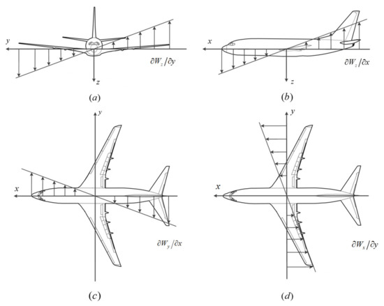
Figure 1.
Schematic diagrams for the gradients of the velocity components: (a) the gradient of vertical wind speed along the lateral axis. (b) the gradient of vertical wind speed along the longitudinal axis. (c) the gradient of lateral wind speed along the longitudinal axis. (d) the gradient of longitudinal wind speed along the lateral axis.
2.2. Building the Influence Coefficient Matrix
As the first step of the vortex lattice method, the surface of the lifting body should be assigned by vortex lattices. Compared with a horseshoe vortex, vortex rings can be distributed on the mean camber surface of the wing to further improve the computing accuracy. The vortex ring assignment facilitates the unsteady aerodynamics analysis in wind disturbance as well. To obtain the aircraft response to the wind gradients, the fuselage is assumed to be cruciform, which is composed of a horizontal plane and a vertical plane. As far as the control surfaces are concerned, the boundary of the vortex lattice should be designed to accord with the structural boundary of the control surfaces. Therefore, the change in aerodynamic force due to the deflection of control surfaces can be computed with better accuracy and separated from the turbulence-induced force change. The division of the vortex lattices on the whole aircraft is shown in Appendix A, Figure A1 and Figure A2.
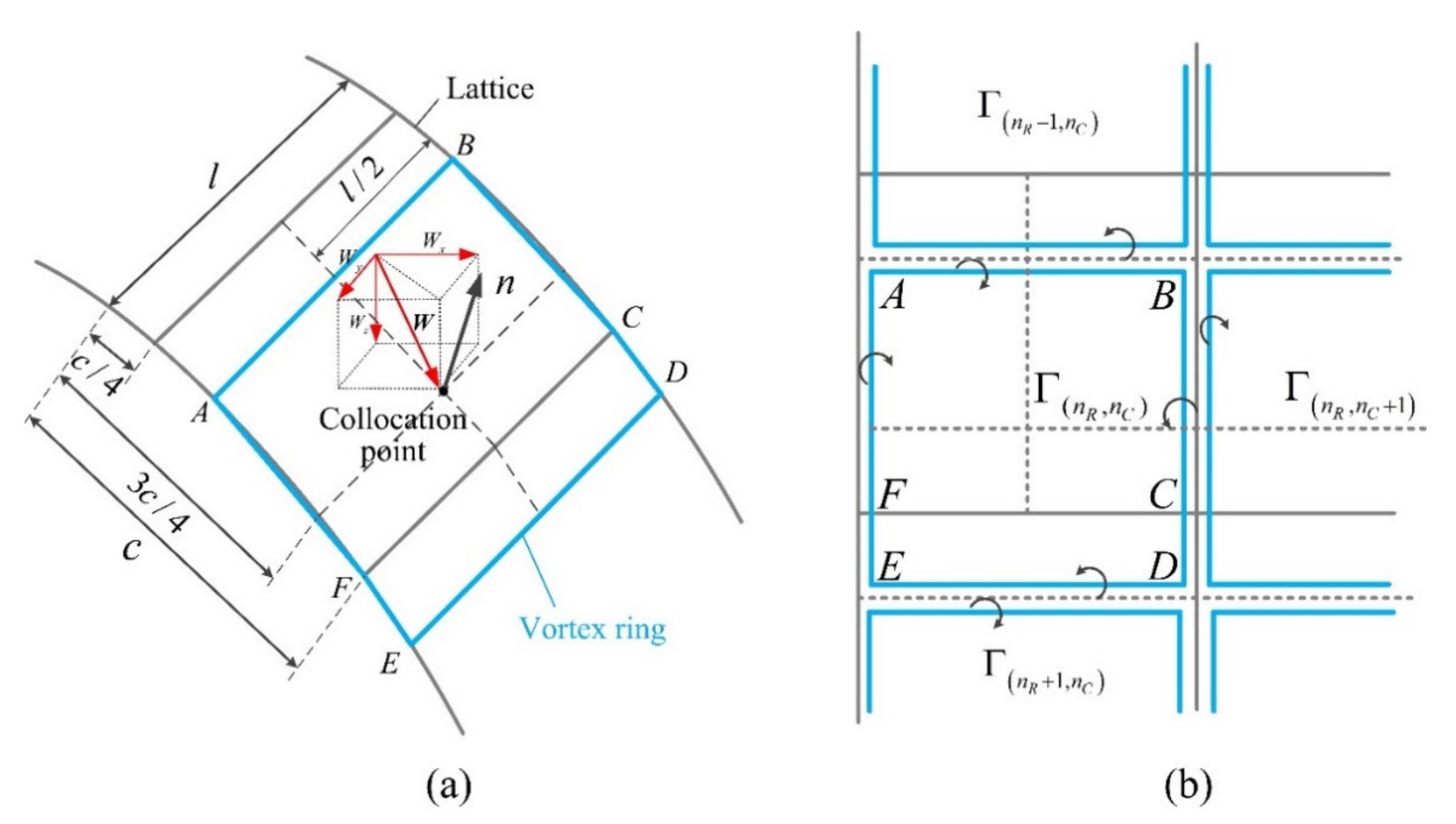
According to the theory of linear-field approximation, the wind gradients make the turbulence components variate on different locations of the aircraft. As shown in Figure 2a, to compute the aerodynamic force induced by the wind components in a specific location, vortex filament AB is assigned on the quarter chord of the vortex lattice, and the vortex ring ABCDEF is closed by connecting six endpoints. The collocation point of each vortex ring locates at the midpoint of the 3/4 chord. The induced velocity at an arbitrary point is determined by the Biot–Savart theorem [17]. When it comes to the closed vortex ring, the induced velocity at the arbitrary point is the linear superposition of the velocity induced by six sections of the vortex filaments. As a result, the total induced velocity depends on the circulation of the vortex ring and an induced coefficient vector (ICV) as

Figure 2.
The vortex ring layout: (a) the vortex ring arrangement and wind speed components on collocation point. (b) the neighboring rings for a general vortex ring.
Once the cruciform layout of vortex lattices is determined for the target aircraft, the ICV of the j-th vortex ring at i-th collocation point is obtained. Furthermore, an induced coefficient matrix (ICM) is obtained as
where is the total number of lattices on the horizontal and lateral plane of the fuselage, the wing, and the horizontal and vertical tail. Since is exclusively determined by the geometrical parameters of the vortex lattices, it can be computed in advance.
2.3. Aircraft Acceleration Response in Turbulence
2.3.1. Local Velocity Induced by Aircraft Unsteady Motion
In turbulent flight, the local velocity at each collocation point is induced by the algebraic sum of the free-flow from far-field, aircraft roll, pitch, and yaw motion, and instantaneous turbulence. As shown in Equation (7), instantaneous wind components on each collocation point are computed based on the wind components at the gravity center and the wind gradients
where represents the coordinate of the gravity center, is the coordinate of arbitrary collocation point; and represents the roll, pitch, and yaw angular velocity of aircraft, respectively.
2.3.2. Computing Unsteady Aerodynamic Force
According to the Neumann boundary condition, the normal component of the local velocity should be equal to zero at each collocation point. The boundary condition is described by
where is the local velocity, represents the induced velocity of the aircraft-attached vortex, while is the circulation of each vortex ring. is the induced velocity of the unsteady wake vortex at each collocation point. There is no wake vortex initially, thus the in Equation (8) equals zero. The initial circulations of the vortex rings are obtained by solving Equation (8) without the wake system.
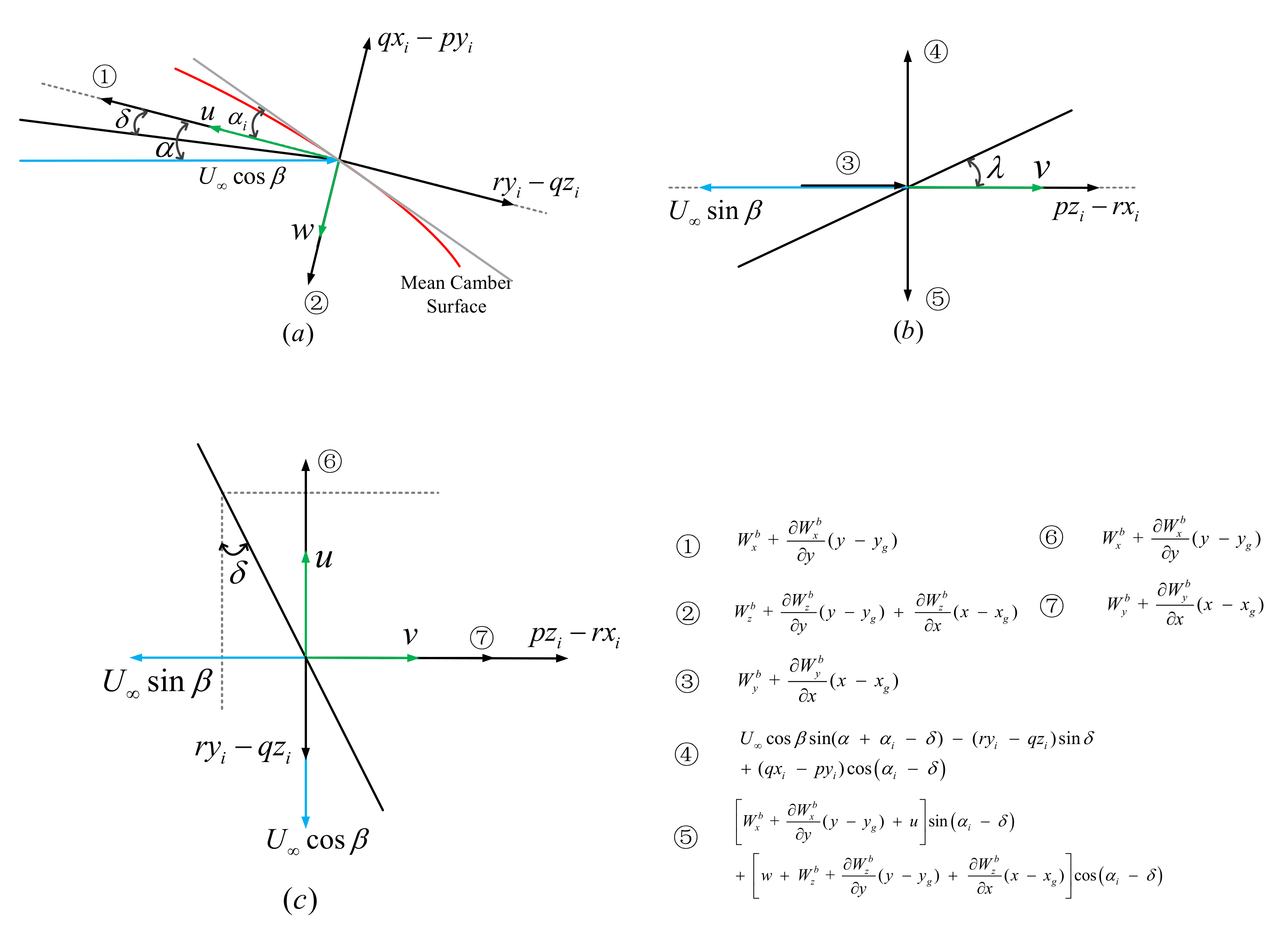
To further study the wind gradients and aircraft maneuvers effects on the acceleration response, the boundary condition is further decomposed on a specific collocation point, as shown in Figure 3. A side view of the boundary condition for the horizontal lifting panel is shown in Figure 3a. A general description of the collocation point on the wing, horizontal tail, and horizontal plane of the fuselage is
where is the increment of angle of attack caused by the deflections of the control surfaces. equals zero on most of the lifting panel without control surfaces. shows the camber effects of the airfoil, and it equals zero on the horizontal plane of the fuselage. are the induced velocity components induced by both the aircraft-attached vortex and the wake vortex.
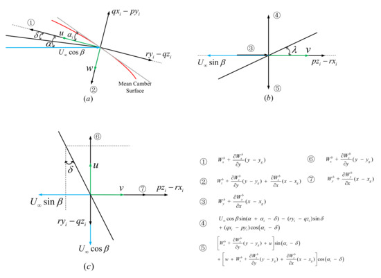
Figure 3.
Decomposition of the turbulent boundary conditions: (a) the side view of the boundary condition for the horizontal lifting panel. (b) the front view of the boundary condition. (c) the boundary condition for the vertical plane of the cruciform assembly.
Figure 3b shows the front view of the boundary condition. The dihedral angle of the wing or horizontal tail changes the boundary condition, thus Equation (9) is modified further as
For the vertical plane of the cruciform assembly, as shown in Figure 3c, the boundary conditions at the collocation point of the vertical plane are decomposed by
where is the deflection angle of the control surface, such as the rudder. It equals zero for most of the vertical panel.
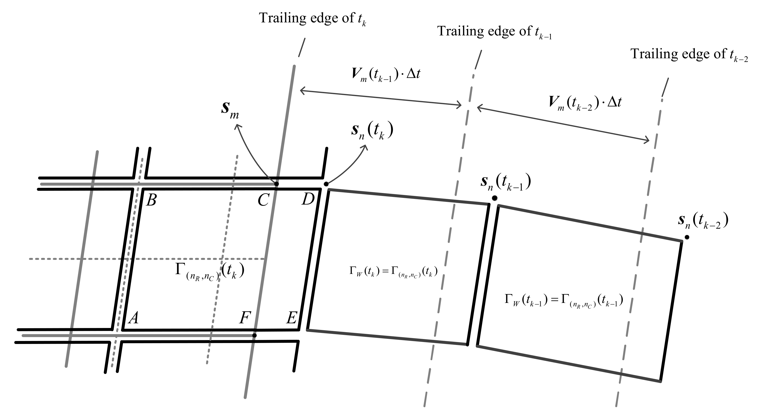
In the process of unsteady motion, wake vortices are generated continuously along the flight trajectory. Thus, the local velocity at each collocation point is affected by wake vortices as well. At each time step , the vortices on the trailing edge of the lifting panel leaves with invariant circulation. In this way, the Kutta condition of at the trailing edge is satisfied [27]. An explicit unsteady flowing process of the wake vortex is shown in Figure 4. Points C and F represent the structural boundary of the trailing edge, and their current location can be described by . The corner point of the first wake vortex, represented by D and E, are determined as

Figure 4.
The schematic diagram of the unsteady wake vortex process.
In Equation (12), is the local velocity of the boundary point at a previous time step, and it can be computed by
where is the induced velocity of the aircraft-attached vortex at the boundary point, is the local velocity, and is the induced velocity of the wake vortex. During the time steps, the corner points move forward with , and a column of wake vortices is generated repeatedly. The circulations of the wake vortices remain unchanged once leaving the trailing edge, thus leading to the determined circulation of the wake vortices. Furthermore, the wake vortices are not affected by aerodynamic force and move forward with local velocity. In addition, the corner points of each wake vortex should be corrected in each time step by
After computing the positions of the wake vortices at any time step, the ICV and ICM can be obtained. Based on the circulations of the wake vortices, the induced velocity of the wake vortex system at any collocation point can be obtained. In practice, the wake vortices locating far away from the trailing edge (more than 20 times of the wing span) are ignored.
2.3.3. Aerodynamics Response with Air Compressibility Correction
By solving Equation (8), the circulation distribution of the whole aircraft is obtained. The aerodynamic force can be further calculated based on the Kutta–Joukowski theorem [20]. As shown in Figure 2b, the vortex filaments of the adjacent vortex rings need to be superimposed to obtain the actual circular distribution. Taking the wing of the right-hand side, for instance, the aerodynamic force at each collocation point in the incompressible flow is:
where is the atmospheric density. Since there is no vortex ring in front of the leading edge for all the lifting surfaces, equals zero on the leading edge. As far as the trailing edge is concerned, does not exist since the vortex filament of the CD segment is not on the lifting surface.
During the high-subsonic cruising flight of civil aviation aircraft, the effects of air compression on aerodynamic force cannot be neglected. Thus, the aerodynamic response needs to be corrected in high-subsonic flight as well. As far as the high-subsonic flow (M > 0.7) is concerned, the pressure coefficient in compressible flow is corrected by the Karman–Tsien rule [18]. Based on the linearized velocity potential equation with incompressible flow, the aerodynamic force of Equation (15) is corrected by
At each time step, the aerodynamic force with and without turbulence should be computed separately, which are recorded as and . In other words, to separate the aerodynamic force change induced by the control surface deflections, the total aerodynamic force is computed twice. By subtracting from , the incremental aerodynamic force caused by turbulence is obtained. As a result, by summing up the aerodynamic force on all of the collocation points, the total aerodynamic force and the force without turbulence effects are obtained successively. Thus, the change in aerodynamic force only induced by turbulence is obtained by . Furthermore, the acceleration change in turbulence is obtained by integrating the following equations:
By integrating Equation (17), the acceleration change is only caused by turbulence, with aircraft maneuvers eliminated. Unlike the wing-tail assembly, with the fuselage and vertical tail considered, the cruciform assembly holds promise to obtain a more accurate acceleration response.
To obtain the wind components at different locations, the change in the wind gradients needs to be computed at each sampling time of the flight data. First, the change in aircraft position is obtained by integrating the following equations [28]:
Based on the wind components obtained at each time step and the position change of the aircraft, the four wind gradients are computed as follows:
A proposed algorithm flow is shown in Figure 5. The cruciform assembly of the vortex lattices is built beforehand. After that, the ICV and ICM are computed. In an algorithm loop, three wind components are computed based on flight data input. The algorithm loop involves the local velocity computation, wake vortex generation, and air compressibility correction. In addition, the wind gradients are obtained by updating the aircraft position. Thus, the vertical acceleration of the aircraft is computed based on the linear-field approximation. The aerodynamic force with and without turbulence are computed, separately, to solve the change in aerodynamic force . In the end, aircraft acceleration is obtained, in which the vertical components can be used to estimate the EDR value.
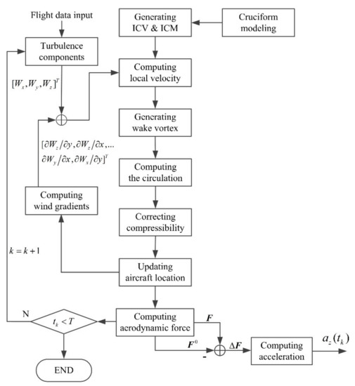
Figure 5.
The flowchart of the proposed algorithm.
3. Results and Discussion
3.1. Aerodynamic Performance Verification by UVLM
Instead of a polynomial fitting function and linear transfer function, the UVLM was used for acceleration estimation in this study; thus, the performance of the UVLM was tested as a basis for further acceleration response analysis. The refined aerodynamic performance can be obtained with a certain number of vortex lattices on the lifting panel [6]. Therefore, under the premise of ensuring the computing accuracy, an appropriate grid resolution to improve the computing efficiency was studied at first.
A Boeing 737 aircraft and related QAR flight data were used for testing in this study. Based on the grid refinement study, the optimized number of vortex lattices of each part of the aircraft is shown in Table 1.

Table 1.
The number of vortex lattices on each part of the aircraft.
Although there is a gap in the aerodynamic performance between the real aircraft and the cruciform assembly, this study focuses on the aerodynamic change induced by turbulence or aircraft maneuvers, rather than obtaining the aerodynamic performance of the whole aircraft. Based on the wing-tail assembly, the computation results of the pitching moment change due to the deflection of the elevator and stabilizer, as analyzed in [29]. It is proved that the computation results by UVLM approximate the modeling data. With the cruciform fuselage added to the wing-tail assembly, this study further tested the lateral aerodynamics change due to the deflection of the spoilers.
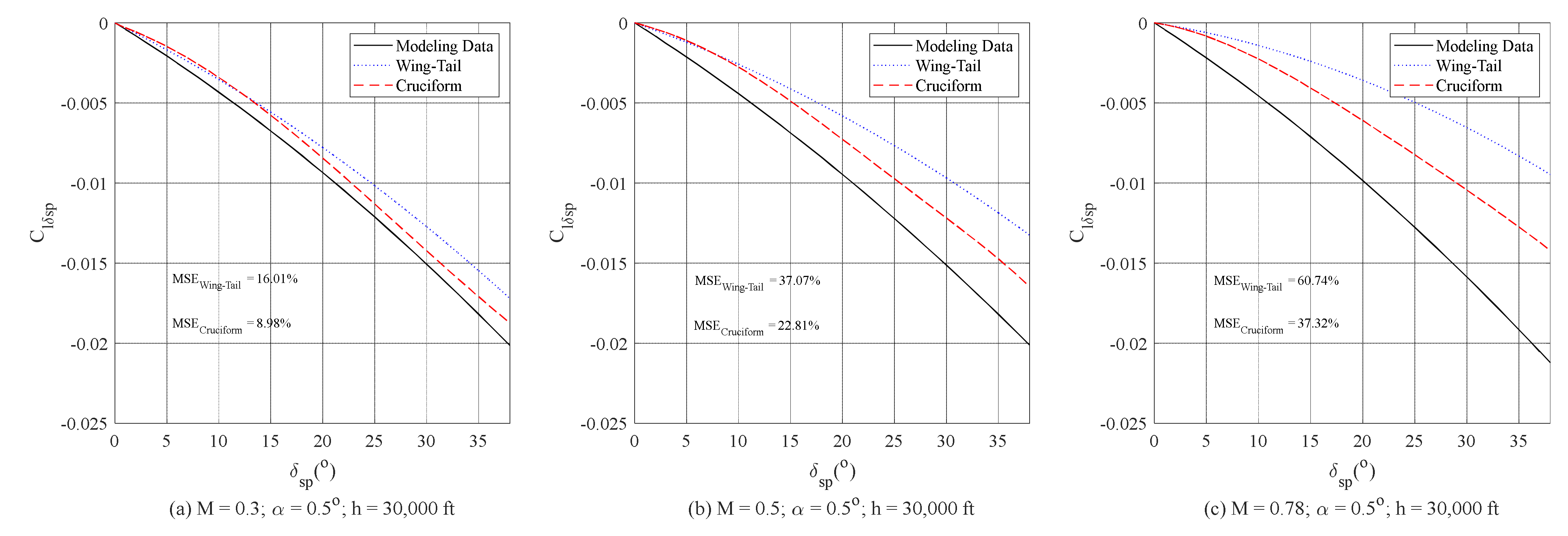
Figure 6 shows the rolling moment change due to the deflection of the high-speed spoilers in three flight states. Comparisons were conducted among the authentic modeling data (Modeling data) [30,31], VLM results with wing-tail assembly (Wing-Tail), and that with the cruciform assembly (Cruciform). Results indicate that the computed rolling moment with the cruciform assembly approximates the modeling data better than that with the wing-tail assembly. However, with the increase in Mach number, the computed results of the cruciform assembly deteriorated because of the air compression.
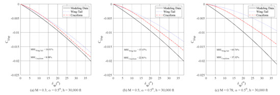
Figure 6.
Comparison of the computation and experimental rolling moment coefficients: (a) in the flight states of M = 0.3, , and h = 30,000 ft; (b) in the flight states of M = 0.5, , and h = 30,000 ft; and (c) in the flight states of M = 0.78, , and h = 30,000 ft.
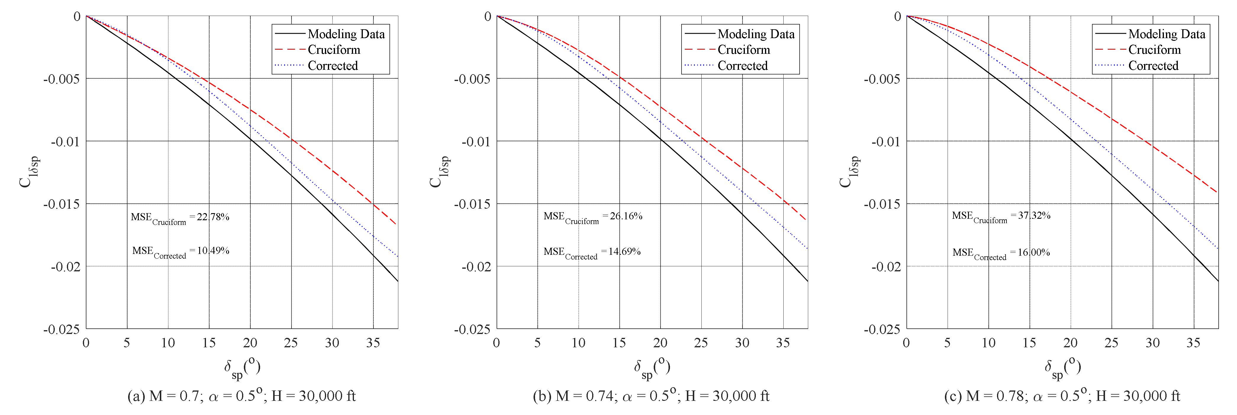
In high-subsonic flight (M > 0.7), the air-compression effects on aerodynamics performance cannot be neglected. The error of the computed rolling moment derivatives increased without air-compression correction. In this study, the air-compression effects in high-subsonic flight were compensated for in the UVLM. Three tests at M = 0.7, M = 0.74, and M = 0.78 were carried out, as shown in Figure 7. With the compression effects corrected, the computed UVLM approximated the modeling data much better.
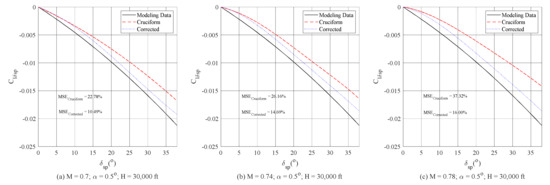
Figure 7.
Comparison of the computation and experimental rolling moment coefficients in high-subsonic flight: (a) in the flight states of M = 0.7, , and h = 30,000 ft; (b) in the flight states of M = 0.74, , and h = 30,000 ft; and (c) in the flight states of M = 0.78, , and h = 30,000 ft.
The above tests proved that based on the UVLM with cruciform assembly, the aerodynamic performance changes due to control surface deflections is computed satisfactory for the aim of this study. The accurate UVLM with cruciform assembly provides a good basis for further estimating aircraft acceleration. In addition, the accurate influence analysis of the control surface deflections is of great significance for separating the effects of aircraft maneuvers on EDR estimation.
3.2. Vertical Acceleration Response
The acceleration response to turbulence was analyzed and further compared with the measured acceleration recorded in the QAR flight data. With the support of Chinese airlines, QAR flight data for 400 flight segments were collected from Boeing 737 aircraft on the same flight route.
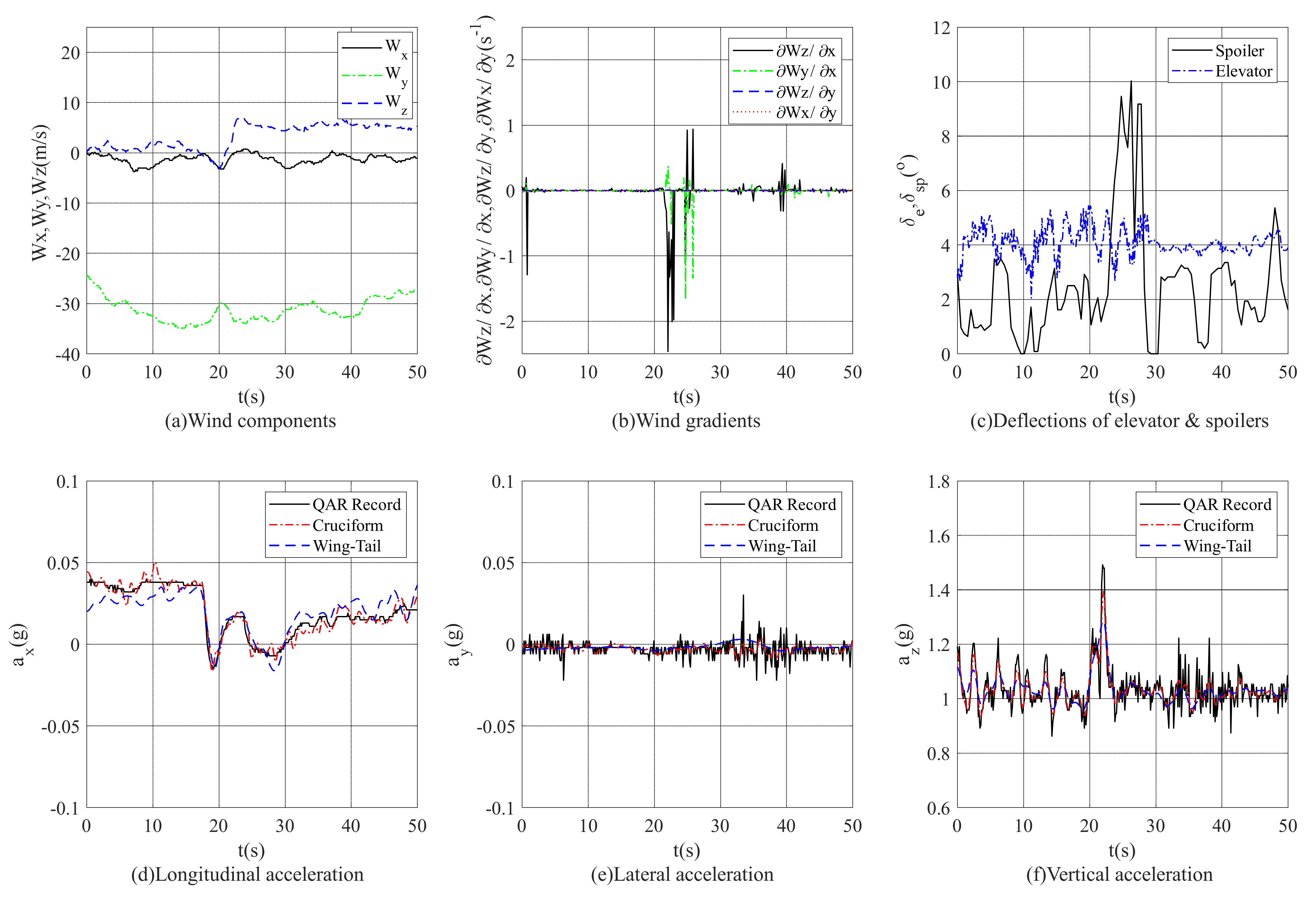
In this section, a flight section with large lateral wind was used for the analysis. As shown in Figure 8, a flight segment of 50 s with large lateral wind and moderate turbulence was used for vertical acceleration analysis. Three curves of wind components are shown in Figure 8a, in which the wind component showed the aircraft was experiencing large lateral wind. Four derived wind gradients, , , , and , are shown in Figure 8b. The deflections of the elevators and spoilers are shown in Figure 8c, in which the deflection of the spoilers reached 10° at 26.5 s. Figure 8d–f shows the computed and recorded acceleration data on the longitudinal, lateral, and vertical axis respectively.
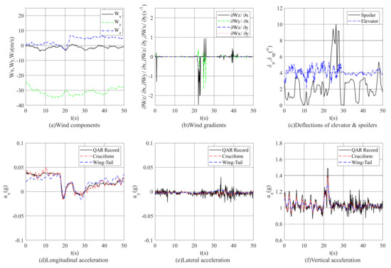
Figure 8.
Aircraft response to turbulence with a large lateral component: (a) the three-axis wind speed components; (b) the four derived wind gradients; (c) the deflections of the elevators and spoilers; (d) the computed and recorded acceleration data on the longitudinal axis; (e) the computed and recorded acceleration data on the lateral axis; (f) the computed and recorded acceleration data on the vertical axis.
The computation results of the UVLM with a cruciform assembly better approximates the recorded acceleration data. The accurate acceleration components confirmed that the derivation of the total aerodynamic force is accurate. When it comes to the UVLM with wing-tail assembly, only the vertical acceleration approximated the recorded QAR data since the UVLM with wing-tail assembly was capable of computing the longitudinal performance much better than the lateral performance.
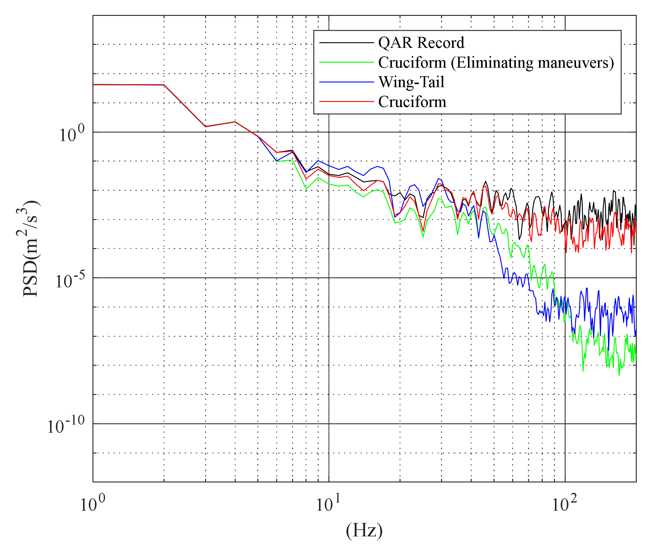
The spectra of the computed acceleration and recorded values are compared as shown in Figure 9. In order to obtain the spectrum densities of the vertical acceleration series, the Welch spectrum density estimation with the Hanning-window function was used [32]. The time-domain data length of each curve was 2560 points, representing the acceleration data length of 640 s. Based on the sampled acceleration data with a sampling rate 4 Hz, the window length was 10 × fs = 40, and the overlapping was set by 50%. Compared with the uniform-wind assumption, the spectrum density of the linear-field approximation approximated the recorded data much better in the high-frequency section. It showed that the UVLM with cruciform assembly is able to track the fluctuation better in the high-frequency domain. However, with aircraft maneuvers eliminated, the total energy of the acceleration spectra is smaller than that of the recorded acceleration. It can be concluded that the vertical acceleration change is not only induced by turbulence, but also affected by aircraft maneuvers; in other words, the deflections of the control surfaces. Since the boundary of the vortex lattice was designed to approximate the structural boundary of the control surfaces, the acceleration induced by aircraft maneuvers can be separated from that induced by turbulence.
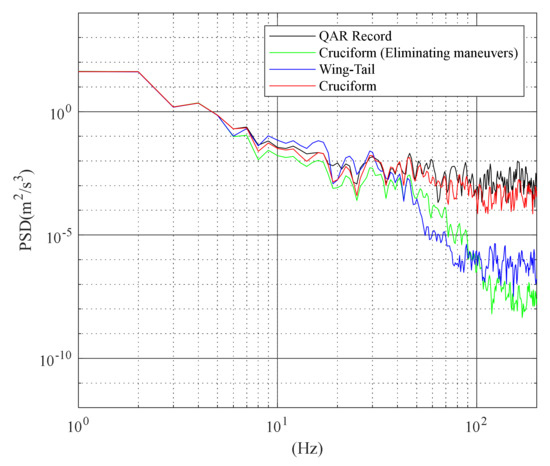
Figure 9.
Comparisons of the acceleration spectrum.
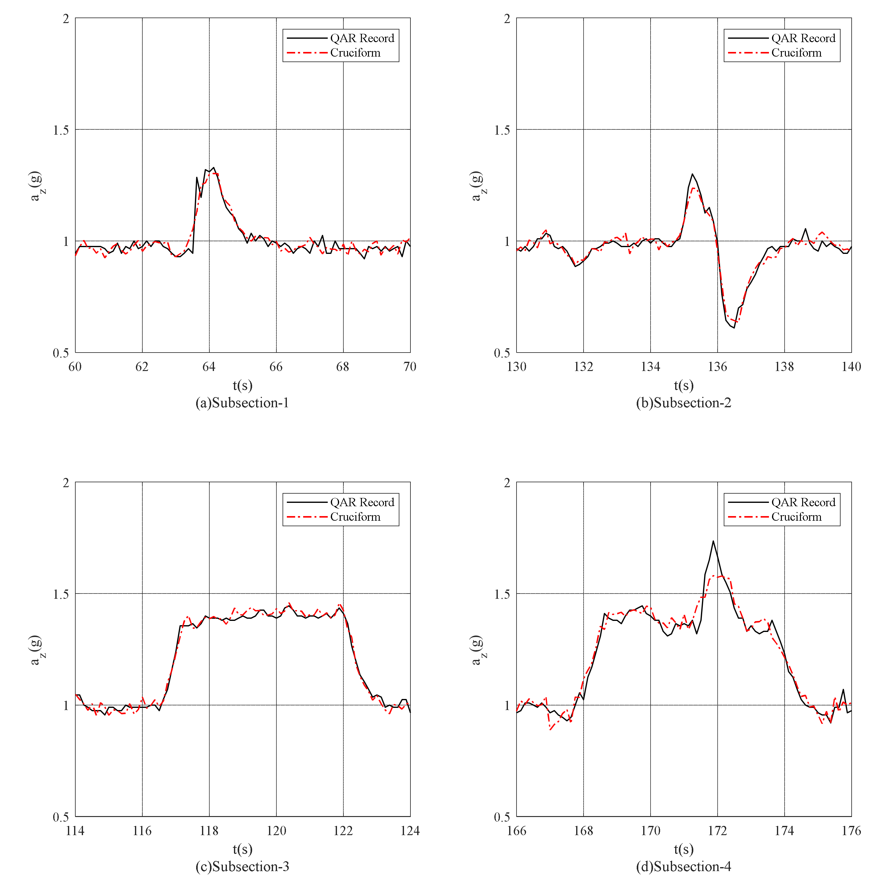
Another flight segment in severe turbulence was used for vertical acceleration analysis in the time domain. As shown in Figure 10, four subsections of vertical acceleration data were used for comparison.
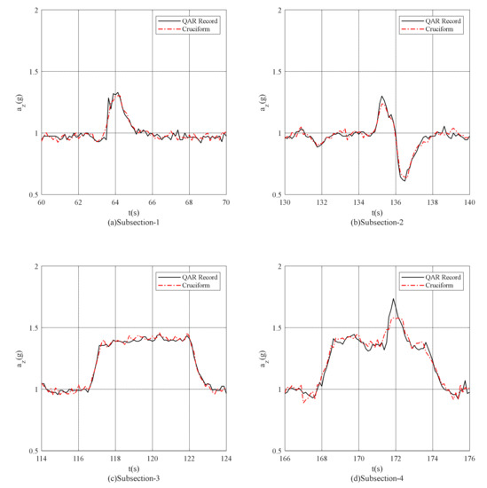
Figure 10.
Record and calculated vertical acceleration response: (a) the comparison between the recorded acceleration and the computations results in subsection-1; (b) the comparison between the recorded acceleration and the computations results in subsection-2; (c) the comparison between the recorded acceleration and the computations results in subsection-3; (d) the comparison between the recorded acceleration and the computations results in subsection-4.
Figure 10a–d is a short-time comparison between the recorded acceleration and the computations results. As shown in Figure 10a, up to 62.5 s, the vertical acceleration was around 1 g, implying the aircraft was at a trimmed flight condition. The maximum positive acceleration rose up to 1.32 g at 64 s. After that, it experienced a continuous decrease and returned to the trimmed flight condition approximately. The computation results tracked the change in acceleration across the entire time span. In Figure 10b, the vertical load reached 1.3 g at 135 s, and then experienced a rapid descent to 0.6 g in one second. Compared with the tracking process shown in Figure 10a, the recommended algorithm maintained stable tracking in case of a wide-range transition of acceleration. The instantaneous tracking ability was acceptable. Figure 10c showed a continuous severe overload of 1.4 g from 116.5 s to 121.8 s. The computation results are consistent with the recorded QAR data. Figure 10d shows a continuous bumpiness. The aircraft reacted to the initial disturbance at 167.5 s and then reached the local maximum load after about 2 s. The maximum load 1.72 g appeared at 171.8 s, and then the acceleration started to decrease. After the overload retention of about 1 s, it experienced a continuous decrease from 173.5 s. During the long time span of overload, the computation results tracked the instantaneous change in acceleration well.
The above four curves represent several typical characteristics in turbulent flight. The UVLM with cruciform assembly exhibited a global tracking ability to the change of vertical acceleration. In addition, the integration of the wind gradients avoided the overshoot in the tracking process.
3.3. Application on EDR Estimation
The analysis of acceleration response in Section 3.2 is composed of two parts. One is induced by turbulence, while the other is induced by control surface deflections, also known as aircraft maneuvers. The two parts can easily be separated by computing the UVLM twice in the algorithm loop. Since the objective EDR estimation requires the acceleration response only induced by turbulence, the adverse effects of aircraft maneuvers must be eliminated in computing the acceleration response by cruciform assembly. Both the acceleration-based and wind-based EDR estimation in [6] were cited in this study.
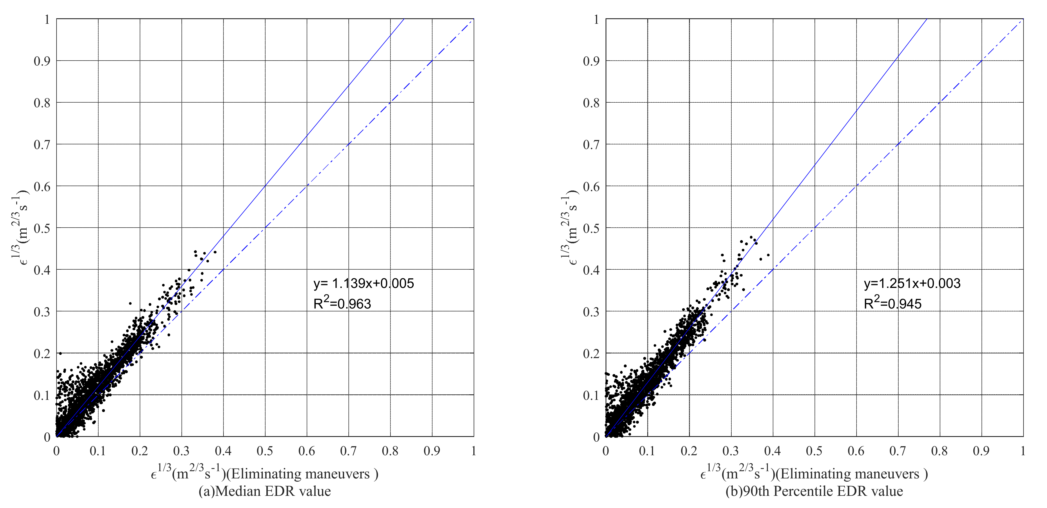
Based on the QAR flight data of 400 flight segments, Figure 11 shows a scatterplot of the total 2000 EDR values for acceleration-based EDR estimation. Figure 11a shows the scatterplot of the one-minute median EDR values, whereas Figure 11b shows the 90th percentile EDR values. For each point, the vertical coordinate represents the EDR value based on the obtained total aerodynamic force , and the horizontal coordinate represents the EDR value based on the . If the two estimation results output the same aircraft-independent EDR value, the estimated EDR value should distribute on the one-to-one straight line, which is clearly identified by y = x in Figure 11. However, a number of points were clustered above the one-to-one line. These overlying points were due to the effects of maneuver-induced accelerations. A first-order fitting function was applied to the data points, with the fitting equation y = 1.1391x + 0.0050 and the correlation coefficient 0.96347. It means that aircraft maneuvers contaminated the EDR estimation results. For the 90th percentile values, the fitting function was y = 1.2511x + 0.0035 and the correlation coefficient was 0.9449. It means that the discrete sudden bumpiness made the 90th percentage EDR value unchanged. Results indicate that the proposed method can better eliminate the influence of aircraft maneuvering flight in EDR estimation, as the first-order function has a bigger slope both in the median and 90th percentile EDR values. The UVLM with cruciform assembly shows a desirable acceleration response all over the spectrum range of the acceleration.
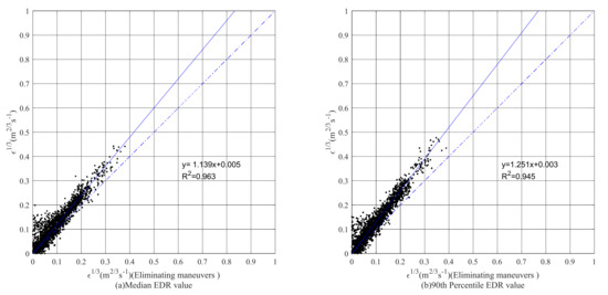
Figure 11.
The comparison of the derived EDR value: (a) the scatterplot of the one-minute median EDR values. (b) the scatterplot of the 90th percentile EDR values.
A further comparison of acceleration-based and wind-based EDR estimation is shown in Figure 12. With the increase in turbulence intensity, the number of outliers in the 90th percentile EDR estimation increased. The variance in EDR values by wind-based method increases because the outliers increases, as shown in Figure 12a. Benefitted by the accurate computation of vertical acceleration, the number of outliers by acceleration-based EDR estimation is much less than the wind-based method, as shown in Figure 12b. The fitted curves in Figure 12a,b reflect the concentration of the EDR estimation. With the cruciform assembly and linear-field approximation, the estimation stability of the acceleration-based method is better than that of the wind-based method.
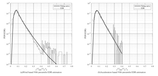
Figure 12.
The comparison of acceleration-based and wind-based EDR estimation: (a) the PDF of the wind based 90th percentile EDR estimation. (b) the PDF of the acceleration based 90th percentile EDR estimation.
4. Conclusions
An accurate estimation of the vertical acceleration response to atmospheric turbulence is fundamental to acceleration-based EDR estimation. Compared with small-scale turbulence at a high altitude, the dimension of a civil aviation aircraft is comparable to the wind field; thus, the linear wind field with the wind gradients effects is preferable to describe the turbulence effects. This study proposes a method of vertical acceleration estimation based on the unsteady vortex lattice method with cruciform assembly. Some innovations are as follows:
(1) The cruciform assembly of the vortex lattices was proposed to analyze the aerodynamic performance in turbulent flight with linear-field approximation. In addition to the non-planar vortex lattices assigned on the wing and horizontal tail assembly, the fuselage was described by cruciform vortex lattices. The turbulence change in different locations of the aircraft was computed by considering the effects of the wind gradients.
(2) The lattices neighboring to the control surfaces, such as the ailerons, spoilers, and elevators, were revised to approximate the structural edge. Thus, the adverse effects of aircraft maneuvers can be separated from the turbulence-induced acceleration change. The separation of aircraft maneuvers is beneficial for acceleration-based EDR estimation.
(3) The influence of air compression in high-subsonic flight of a civil aviation aircraft was compensated for by the Karman–Tsien rule in the UVLM. The accuracy of the aerodynamic force is further improved in high-subsonic turbulent flight.
Compared with the wing-tail assembly, the cruciform assembly with wind gradient effects has better accuracy in computing the acceleration response, especially the lateral response. The vertical acceleration response only induced by turbulence is obtained for acceleration-based EDR estimation. Furthermore, with the optimized acceleration response, the process of EDR estimation eliminates the adverse effects of aircraft maneuvers effectively and has got better accuracy and stability.
This paper is the first attempt to apply the linear turbulence field approximation on the estimation of aircraft acceleration response and EDR estimation. In the future, the lattices layout and related vortex rings on the fuselage will be refined to further improve the computing accuracy. In addition, the air compressibility effects should be better compensated for high-subsonic flight.
Author Contributions
Conceptualization, Z.G.; methodology, D.W., Z.G. and H.G.; software, D.W. and. Z.G.; validation, D.W., H.G. and X.G.; formal analysis, X.G.; investigation, Z.G.; resources, Z.G.; data curation, Z.G.; writing—original draft preparation, D.W.; writing—review and editing, Z.G., H.G. and X.G.; visualization, X.G.; supervision, Z.G.; project administration, Z.G.; funding acquisition, Z.G. All authors have read and agreed to the published version of the manuscript.
Funding
This research was funded by Natural Science Foundation of China, Grant Number [NSFC: U1733122, U1533120].
Institutional Review Board Statement
Not applicable.
Informed Consent Statement
Not applicable.
Data Availability Statement
Not applicable.
Conflicts of Interest
The authors declare no conflict of interest.
Appendix A
This appendix describes the grid division of the cruciform assembly in detail. To obtain the aircraft response to turbulence with wind gradient effects, the fuselage was simplified to be cruciform. The vertical plane, described by two trapezoidal zones, Zone I and Zone II, had 1600 vortex lattices. The lattices on the vertical plane are divided equally; thus, Zones I and II have got the same number of columns. In addition, the horizontal plane, simplified by two symmetrical trapezoids, Zones III and IV, has 1400 vortex lattices. The equal-distance partition method was used to divide the lattices as well.
As shown in Figure A2, the vortex lattices on the wing were distributed on the mean camber surface to improve the computing accuracy further. The wing of a civil aviation aircraft was generally divided by two sections on each side, Zone V and Zone VI, with different sweep back angles at the trailing edge. The vortex lattices were assigned on each zone, in which the column was divided based on the equal-angle partitioning method, while the lattice intervals along the chord-direction were identical. The horizontal tail was divided into Zones IX and X and the vertical tail was labeled as Zone XI. There are in total 1600 lattices on the wing, 360 lattices on the vertical tail, and 320 lattices on the horizontal tail. Thus, in the cruciform assembly, the whole aircraft is composed by eleven zones and the total number of lattices is 5280.
When it comes to the control surfaces, such as the elevator, spoilers, and ailerons, the boundary of the vortex lattice should coincide with the structural boundary of the control surfaces. In this way, the aerodynamic force change due to the deflection of the control surfaces is able to be computed with better accuracy. Furthermore, since all the vortex lattices must be closed, the contact edge of each part of the aircraft must be modified to align with the boundary of the vortex lattice. After dividing the lattices, the coordinate of each collocation point can be computed based on the geometric parameters.
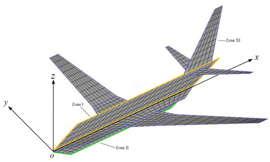
Figure A1.
The cruciform assembly of the aircraft.
Figure A1.
The cruciform assembly of the aircraft.

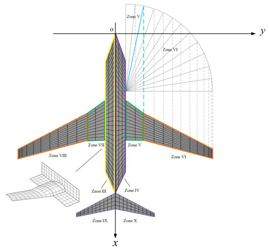
Figure A2.
Grid division of the wing.
Figure A2.
Grid division of the wing.

References
- Sharman, R.; Lane, T. Aviation Turbulence; Springer: Cham, Switzerland, 2016; Volume 10, pp. 978–983. [Google Scholar]
- Gao, Z.X.; Fu, J. Research on Robust LPV modeling and control of aircraft flying through wind disturbance. Chin. J. Aeronaut. 2019, 32, 1588–1602. [Google Scholar] [CrossRef]
- Barleben, A.; Haussler, S.; Müller, R.; Jerg, M. A Novel Approach for Satellite-Based Turbulence Nowcasting for Aviation. Remote Sens. 2020, 12, 2255. [Google Scholar] [CrossRef]
- Kim, J.H.; Park, J.R.; Kim, S.H.; Kim, J.; Lee, E.; Baek, S.; Lee, G. A Detection of Convectively Induced Turbulence Using In Situ Aircraft and Radar Spectral Width Data. Remote Sens. 2021, 13, 726. [Google Scholar] [CrossRef]
- Guo, J.; He, J.X.; Hu, C.J.; Wu, J.Y. Analysis of Wind Induced Vibration of Stayed Cable of Sea-crossing Bridge Based on Monitoring Data. EASEC16: Proceedings of the 16th East Asian-Pacific Conference on Structural Engineering and Construction, Brisbane, Australia, 6–9 December 2019; Springer: Singapore, 2021; pp. 187–198. [Google Scholar]
- Gao, Z.; Wang, H.; Qi, K.; Xiang, Z.; Wang, D. Acceleration-Based in Situ Eddy Dissipation Rate Estimation with Flight Data. Atmosphere 2020, 11, 1247. [Google Scholar] [CrossRef]
- Kim, S.H.; Chun, H.Y.; Kim, J.H.; Sharman, R.D.; Strahan, M. Retrieval of eddy dissipation rate from derived equivalent vertical gust included in Aircraft Meteorological Data Relay (AMDAR). Atmos. Meas. Tech. 2020, 13, 1373–1385. [Google Scholar] [CrossRef] [Green Version]
- Etkin, B. Turbulent wind and its effect on flight. J. Aircr. 1981, 18, 327–345. [Google Scholar] [CrossRef]
- Podglajen, A.; Bui, T.P.; Dean-Day, J.M.; Pfister, L.; Jensen, E.I.; Alexander, M.J.; Hertzog, A.; Kärcher, B.; Plougonwen, R.; Randell, W.J. Small-Scale Wind Fluctuations in the Tropical Tropopause Layer from Aircraft Measurements: Occurrence, Nature, and Impact on Vertical Mixing. J. Atmos. Sci. 2017, 74, 3847–3869. [Google Scholar] [CrossRef]
- Kimberlin, R.D.; Sims, J.P. Gust Alleviation for General Aviation Aircraft; SAE Technical Paper; SAE International: Warrendae, PA, USA, 1996. [Google Scholar]
- Wright Patterson Air Force Base. Flying Qualities of Piloted Airplanes; MIL-F-8785C; U.S. Air Force: Dayton, OH, USA, 1980. [Google Scholar]
- Joseph, G.; Golubev, V.V.; Gudmundsson, S. Towards Development of a Dynamic-Soaring, Morphing-Wing UAV. In Proceedings of the AIAA Aviation 2020 Forum, Virtual Event, Reston, VA, USA, 15–19 June 2020. [Google Scholar]
- Cornman, L.B.; Morse, C.S.; Cunning, G. Real-time estimation of atmospheric turbulence severity from in-situ aircraft measurements. J. Aircr. 1995, 32, 171–177. [Google Scholar] [CrossRef]
- Huang, R.; Sun, H.; Wu, C.; Wang, C.; Lu, B. Estimating eddy dissipation rate with QAR flight big data. Appl. Sci. 2019, 9, 5192. [Google Scholar] [CrossRef] [Green Version]
- Billy, K.B.; Brett, A.N. Aircraft Acceleration prediction due to atmospheric disturbances with flight data validation. J. Aircr. 2006, 43, 72–81. [Google Scholar]
- Williams, P.D. Increased light, moderate, and severe clear-air turbulence in response to climate change. Adv. Atmos. Sci. 2017, 34, 576–586. [Google Scholar] [CrossRef] [Green Version]
- Nasir, S.; Javaid, M.T.; Shahid, M.U.; Raza, A.; Siddiqui, W.; Salamat, S. Applicability of Vortex Lattice Method and its Comparison with High Fidelity Tools. Pak. J. Eng. Technol. 2021, 4, 207–211. [Google Scholar]
- Jones, B.R.; Crossley, W.A.; Lyrintzis, A.S. Aerodynamic and aeroacoustic optimization of rotorcraft airfoils via a parallel genetic algorithm. J. Aircr. 2000, 37, 1088–1096. [Google Scholar] [CrossRef]
- Hosangadi, P.; Gopalarathnam, A. Low-Order Method for Prediction of Separation and Stall on Unswept Wings. J. Aircr. 2020, 58, 420–435. [Google Scholar] [CrossRef]
- Oliviu, S.G.; Koreanschi, A.; Botez, R.M.; Mamou, M.; Mebarki, Y. Analysis of the aerodynamic performance of a morphing wing-tip demonstrator using a novel nonlinear vortex lattice method. In Proceedings of the 34th AIAA Applied Aerodynamics Conference, Washington, DC, USA, 13–17 June 2016. [Google Scholar]
- Vicroy, D.D.; Bowles, R.L. Effect of spatial wind gradients on airplane aerodynamics. J. Aircr. 1989, 26, 523–530. [Google Scholar] [CrossRef]
- Süelzgen, Z.; Wüstenhagen, M. Operational modal analysis for simulated flight flutter test of an unconventional aircraft. In Proceedings of the International Forum on Aeroelasticity and Structural Dynamics, Savannah, GA, USA, 10–13 June 2019. [Google Scholar]
- Meddaikar, Y.M.; Dillinger, J.; Klimmek, T.; Krueger, W.; Wuestenhagen, M.; Kier, T.M.; Hermanutz, A.; Hornung, M.; Rozov, V.; Breitsamter, C.; et al. Aircraft aeroservoelastic modelling of the FLEXOP unmanned flying demonstrator. In Proceedings of the AIAA Scitech 2019 Forum, San Diego, CA, USA, 7–11 January 2019. [Google Scholar]
- Meng, Y.; Wan, Z.; Xie, C.; An, C. Time-domain nonlinear aeroelastic analysis and wind tunnel test of a flexible wing using strain-based beam formulation. Chin. J. Aeronaut. 2021, 34, 380–396. [Google Scholar] [CrossRef]
- Zhang, Q.; Liu, H.H.T. Aerodynamics modeling and analysis of close formation flight. J. Aircr. 2017, 54, 2192–2204. [Google Scholar] [CrossRef]
- Parenteau, M.; Sermeus, K.; Laurendeau, E. VLM coupled with 2.5 d RANS sectional data for high-lift design. In Proceedings of the 2018 AIAA Aerospace Sciences Meeting, Kissimmee, FL, USA, 8–12 January 2018. [Google Scholar]
- Katz, J.; Plotkin, A. Low-Speed Aerodynamics; Cambridge University Press: Cambridge, UK, 2001. [Google Scholar]
- Dreier, M.E. Introduction to Helicopter and Tiltrotor Flight Simulation; American Institute of Aeronautics and Astronautics: Reston, VA, USA, 2007. [Google Scholar]
- Gao, Z.; Wang, D.; Xiang, Z. A Method for Estimating Aircraft Vertical Acceleration and Eddy Dissipation Rate in Turbulent Flight. Appl. Sci. 2020, 10, 6798. [Google Scholar] [CrossRef]
- Boeing Company. Aerodynamic Data and Flight Control System Description for the 737-600/-700/-800/-900 Training Simulator; D611A001-vol1, rev H.; Boeing Company: Chicago, IL, USA, 2003. [Google Scholar]
- Boeing Company. Aerodynamic Data and Flight Control System Description for the 737-600/-700/-800/-900 Training Simulator; D611A001-vol3, rev H.; Boeing Company: Chicago, IL, USA, 2003. [Google Scholar]
- Stoica, P.; Moses, R. Spectral Analysis of Signals; Pearson Education: Cranbury, NJ, USA, 2005. [Google Scholar]


Publisher’s Note: MDPI stays neutral with regard to jurisdictional claims in published maps and institutional affiliations. |
© 2021 by the authors. Licensee MDPI, Basel, Switzerland. This article is an open access article distributed under the terms and conditions of the Creative Commons Attribution (CC BY) license (https://creativecommons.org/licenses/by/4.0/).