Abstract
Sea surface wind plays an essential role in the simulating and predicting ocean phenomena. However, it is difficult to obtain accurate data with uniform spatiotemporal scale. A high-resolution (10 km) sea surface wind hindcast around the Korean Peninsula (KP) is presented using the weather research and forecasting model focusing on wind speed. The hindcast data for 39 years (1979–2017) are obtained by performing a three-dimensional variational analysis data assimilation, using ERA-Interim as initial and boundary conditions. To evaluate the added value of the hindcasts, the ASCAT-L2 satellite-based gridded data (DASCAT) is employed and regarded as “True” during 2008–2017. Hindcast and DASCAT data are verified using buoy observations from 1997–2017. The added value of the hindcast compared to ERA-Interim is evaluated using a modified Brier skill score method and analyzed for seasonality and wind intensity. Hindcast data primarily adds value to the coastal areas of the KP, particularly over the Yellow Sea in the summer, the East Sea in the winter, and the Korean Strait in all seasons. In case of strong winds (10–25 m·s−1), the hindcast performed better in the East Sea area. The estimation of extreme wind speeds is performed based on the added value and 50-year and 100-year return periods are estimated using a Weibull distribution. The results of this study can provide a reference dataset for climate perspective storm surge and wave simulation studies.
1. Introduction
Sea surface wind plays an essential role in air–sea interaction, thus influencing ocean dynamics. It significantly affects the occurrence and response to natural and manmade maritime hazards, such as abnormal extreme waves, storm surges, search and rescue efforts, and oil spills. In particular, waves and storm surge prediction are determined by the quality of the sea surface wind data [1,2]. In addition, extreme sea surface wind events significantly affect defense infrastructure, offshore wind power, shipping routes, tourism, and leisure activities; thus, it is imperative to have an accurate long-term sea surface wind dataset to better encapsulate wind variability.
The Korean Peninsula (KP) comprises an indented coastline, many islands, and a complex terrain. Accordingly, there is growing interest in obtaining consistent sea surface wind data with a high spatiotemporal resolution for the region [3,4]. Thus far, there is considerable uncertainty regarding sea surface wind data using ocean prediction and research on the reproduction of past waves and storm surges [5,6]. In situ observation data have been used to represent the region despite spatial inadequacies. A higher spatial coverage can be obtained using a satellite scatterometer; however, this has the disadvantage of irregular spatiotemporal scales. Therefore, many previous studies have turned to reanalysis data as an alternative [7,8,9]. These data are considered quasi-observational for variables such as temperature and wind [10], are generated on a global scale by numerical models, and maintain high accuracy by considering all available observations at the time [11]. This can provide consistent atmospheric coverage over the climate-scale, but it is not possible to extract local wind characteristics over complex terrains. Therefore, dynamic downscaling needs to be performed using reanalysis data as boundary conditions.
The regional climate models (RCMs) have been used to estimate climate variability at a detailed spatiotemporal resolution [12] and many studies have investigated the quantitative added value of dynamic downscaled hindcast [12,13,14,15,16,17,18]. Sea surface wind can be observed using The National Aeronautics and Space Administration (NASA) Quick Scatterometer (QuikSCAT) satellite with a root mean square error (RMSE) less than 2 m·s−1 [19]. Therefore, the added value of the ocean surface wind was evaluated using QuikSCAT. Winterfeldt et al. [20] evaluated the value added to the National Centers for Environmental Prediction and the National Center for Atmospheric Research (NCAR) reanalysis (NCEP/NCAR reanalysis) using the hindcast data of sea surface winds produced in Europe from QuikSCAT Level 2 B 12.5 km swath data. Menendez et al. [21] produced two hindcast datasets over the Mediterranean region by dynamically downscaling NCEP/NCAR reanalysis and European Center for Medium-Range Weather Forecasts (ECMWF) reanalysis (ERA-Interim) data using the Weather Research and Forecasting model (WRF) and found that the hindcast performed better when using ERA-Interim for the boundary conditions. Li et al. [22] produced reanalysis data using a high-resolution the consortium for small-scale model (COSMO) in climate mode (CLM) model with ERA-Interim as a boundary for the Bohai and Yellow Sea areas and verified them via in situ observations and satellite data. Conclusively, each of these studies added value to boundary data in coastal areas with complex topography when considering QuikSCAT data as “True.” After QuikSCAT finished observation, the Advanced Scatterometer (ASCAT) has been widely used to measure sea surface wind speeds and directions. Sivareddy et al. [23] has shown that the daily gridded ASCAT wind product (DASCAT) has a higher accuracy than QuikSCAT data during rainfall. Park et al. [24] evaluated DASCAT provides accurate wind speeds around the KP, with RMSE ≤ 3.5 m·s−1.
Research of the sea surface winds around the KP began with a study that used average monthly sea level air pressure and observed that wind data controlled the distribution of wind stress and curl [25]. Subsequent studies explored model verification by comparing in situ observation data [26,27,28] and satellite data [24,29,30,31,32]. Research on high-resolution sea surface wind estimation has mainly focused on the creation of wind resource maps [4,33,34]. Additionally, a coordinated regional climate downscaling experiment for East Asia was carried out as an international regional climate model inter-comparison project (CORDEX-EA) by focusing on the sea surface winds around the KP at a horizontal resolution of 50 km [35]. The spectral nudging technique was used to produce long-term hindcast data of sea surface winds [20,21,22]. There are many case studies using 3DVAR data assimilation to improve the model initial field around KP [36,37,38]. However, there are few studies that adopted 3DVAR data assimilation to produce climate scale hindcast data [5,39].
Consequently, reliable long-term and homogeneous sea surface wind data in the coastal seas around the KP are limited. The present study aimed to produce and verify long-term hindcast sea surface wind data with high spatiotemporal resolutions with 3DVAR data assimilation. Many regions around the KP have complex topographies and coastlines and high-resolution simulations would add value to the boundary data as mesoscale atmospheric phenomena play a significant role in determining the climate. The Yellow Sea (YS), Korean Strait (KS), and East Sea (ES) regions around the KP were considered in this study [40]. The remainder of this paper is organized as follows: Regional atmospheric hindcast production, in situ data, satellite data, and methodologies are described in Section 2; Section 3 presents the results of the hindcast data compared with satellite data and the estimation of extreme wind speeds. A discussion is presented in Section 4 and summary and conclusions are presented in Section 5.
2. Model and Data
2.1. Regional Atmospheric Hindcast
The WRF with the Advanced Research dynamical solver (WRF-ARW) [41] v.3.7.1 was used to obtain regional hindcast data over the KP. The WRF employs the Arakawa-C horizontal grid and a terrain-following hydrostatic pressure vertical coordinate. The numerical model uses a third-order Runge-Kutta time integration scheme with a time interval of 60 s and the 6th-order centered differencing method was introduced for the advection term. It also preserves the mass, momentum, entropy, and scalar using flux-type diagnostic equations. The model domain covers ~20–50° N, ~110–150° E (Figure 1), the horizontal grid resolution is 436 × 436 grids, with 10 km intervals centered on the KP and 60 vertical layers.
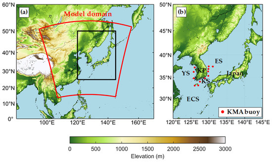
Figure 1.
Orography of the WRF with the Advanced Research dynamical solver (WRF-ARW) domain. (a) Locations of model domain (red quadrangle) and study area (black rectangle). (b) Locations of buoys operated by the Korea Meteorological Administration. YS, KP, ES, ECS, and KS represent the Yellow Sea, Korean Peninsula, East Sea, East China Sea, and Korean Strait.
The atmospheric planetary boundary layer (PBL) plays a crucial role in simulating sea surface winds because it determines the supply of heat, momentum, and moisture from the sea surface to the free atmosphere [42,43] even around the complex coastlines of the KP. A corresponding sensitivity test was performed for four simulations (see supplementary materials for detail). We selected the period from November to December 2015 (High average wind speed and large swell wave event in ES). Physical configuration of each simulation was considered based on Heo et al. [39] and Carvalho et al. [44] (see Table S1). At first, two sets of simulations were performed for the sensitivity test, one using the ERA-Interim as the initial and boundary conditions and the other one using NCEP FNL data. After confirming previous study results that ERA-Interim shows better performance than NCEP FNL [39] (see Figure S1), PBL schemes were evaluated except NCEP FNL based simulations. The Yonsei University (YSU) PBL scheme [45] was adopted, as it showed the best performance (see Figures S2 and S3, Table S2). The WRF single-moment 6-class (WSM6) was used for simulating the microphysics [46], in addition to the rapid radiative transfer model (RRTM) scheme for long-wave radiation and short-wave radiation [47], the Kain–Fritsch scheme [48] for cumulus parameterization, and Noah land surface model scheme [49]. The detailed model specifications are described in Table 1.

Table 1.
Overview of the WRF model configuration for the present analyses of sea surface wind hindcasting around the Korean Peninsula during 1979–2017.
The WRF hindcast data from 1979 to 2017 were obtained from the ERA-Interim reanalysis data. The WRF was reinitialized daily with this data, providing initial and lateral boundary conditions and then run for 30 h. The NCEP daily global sea surface temperature (SST) analysis (RTG_SST_HR) was used to represent the sea surface wind patterns for better accuracy and the 6 h SST data interpolated from RTG_SST_HR were employed as the initial condition. The three-dimensional variational data assimilation (3DVAR) technique was adopted to improve the model’s initial conditions. The 3DVAR had been run every 6 h before 00 UTC. The analysis field is generated by merging observations and background forecasts through iterative minimization of the cost function. NCEP automated data processing (ADP) global air and surface weather observation data and NCEP global data assimilation system (GDAS) satellite data were used as observation data from 1999 to 2017. Before this period, NCEP global telecommunications system (GTS) data were used to determine the optimal initial condition of the WRF. Even with frequent data assimilation, forecast errors dramatically increased with time after each day; therefore, a one-day reinitialization approach was adopted and available observational data were assimilated every 6 h, including the initial hour. The first 6 h of each run was considered to be required for model spin-up and removed from the calculation; data from the remaining one-day periods were combined to create a continuous time series [5]. Most previous studies recommended a spin-up time of 12 h [50]. However, when using the 3DVAR with a similar domain size, spin-up time could be 6 h or shorter [51,52].
2.2. Reanalysis Data
ERA-Interim reanalysis data were adopted as the initial and boundary conditions for obtaining the WRF hindcast data. ERA-Interim is a third-generation reanalysis produced by the European Center for Medium-Range Weather Forecasts (ECMWF) [11]. It covers the period from 1 January 1979 to 31 December 2017. The horizontal spatial resolution of ERA-Interim is approximately 80 km (T255 spectral) with 60 vertical levels. It has been suggested that ERA-Interim has a better performance for wind hindcasts over KP compared to other popular global reanalysis data, such as the global final analysis (FNL) from NCEP [39]. Li et al. [53] compared NCEP reanalysis, NCEP climate forecast system reanalysis (CFSR), Japanese 55-year reanalysis data (JRA-55) as the initial and boundary conditions. ERA-Interim showed best performance in Bohai Sea and YS.
2.3. In Situ Data
In this study, observation data provided by the Korea Meteorological Administration (KMA) were used from 12 meteorological buoys that consistently collected data (Figure 1, Table 2). Wind speed (m·s−1), wind direction (°), gust wind speed (m·s−1), pressure (hPa), humidity (%), air temperature (°C), sea surface temperature (°C), maximum wave height (m), significant wave height (m), average wave height (m), wave period (s), and wave direction (°) are collected and provided 10 min intervals. These data follow the World Meteorological Organization (WMO) standard and it has been observed around the KP from the earliest time beginning in 1997. The KMA buoy data covers the longest period during the research period (Figure 1, Table 2).
Table 2.
Location and observation period of buoy stations.
2.4. Satellite Data
Since the completion of the QuikSCAT mission, ASCAT has been widely used to measure sea surface wind speeds and directions over the ocean surface. ASCAT measurements are based on the Bragg resonant scattering mechanism, for which the backscatter power is directly proportional to the distribution and density of capillary and short gravity waves on the sea surface [54]. In the present study, Level-3 gridded products (DASCAT) that contain wind fields from the L2-swath passes were employed [55] and the objective method was used for interpolation onto a regular grid of 0.25° longitude and latitude. Previous research has shown that the wind observation data obtained through DASCAT has a higher accuracy than QuikSCAT data during rainfall [23]. Moreover, DASCAT provides accurate wind speeds around the KP, with RMSE ≤ 3.5 m·s−1 [24].
2.5. Evaluation Methods
To evaluate the WRF hindcast performance, several statistical parameters were used, including the mean, standard deviation (STD), bias, RMSE, and correlation coefficient (r). Furthermore, the modified Brier skill score (BSS) was used to assess the added value of ERA-Interim using dynamic downscaling described as follows (Equation (1)) [20,56]:
where denotes the square of the error variance of the ERA-Interim reanalysis wind speeds and is the square of the error variance in the WRF hindcast wind speeds compared to DASCAT. The BSS varies between −1 and 1 where a more negative BSS value indicates that ERA-Interim is more consistent with DASCAT and positive BSS values support the added value of WRF hindcast data over the ERA-Interim forcing data. DASCAT is advantageous due to its consistent temporal coverage with ERA-Interim over the study period. Since modified BSS was introduced to evaluate the added value of sea surface wind hindcast [20], many studies used modified BSS to evaluate added value quantitatively [13,21,22,57,58].
3. Results
3.1. DASCAT-Based Assessment of Hindcast Data
The hindcast data for 39 years (1979–2017) were obtained using ERA-Interim as initial and boundary data. DASCAT and KMA buoy data were used for the verification. The data were employed for their available period (2008–2017 for DASCAT and 1997–2017 for KMA buoy). Due to the lack of observation data, DASCAT was considered to be “True” to assess WRF hindcast data, but it was first compared to buoy observation data for validation. DASCAT wind speeds around KP varied between 4.0 and 8.5 m·s−1, with lower values along the coastal area and relatively higher values in the offshore areas. The spatial patterns of wind speed around the KP, East China Sea (ECS), and Kuroshio/Kuroshio Extension were similar to those observed in previous studies [22,35]. The maximum wind speeds in the KS varied from 6.8 to 8.5 m·s−1; in the ES, it varied from 5.6 to 7.2 m·s−1 near the coastal area and from 7.2 to 7.6 m·s−1 in the offshore area; and the YS displayed the lowest wind speed values near the coastal area (4.8 m·s−1) which never exceeded 8 m·s−1, ultimately indicating a wide range of mean wind speeds in each sea area (Figure 2a). The highest wind speeds were observed in the ECS and the Kuroshio/Kuroshio Extension; however, the present study focused on the KP as the region of interest. Wind speed variability was also the greatest over the open sea (Figure 2b). The KS had the highest wind variability in the coastal region (~3.2–3.8 m·s−1) and the offshore area (~3.0–3.6 m·s−1), illustrating that wind speed over the KP was spatially diverse within each sea area as well.
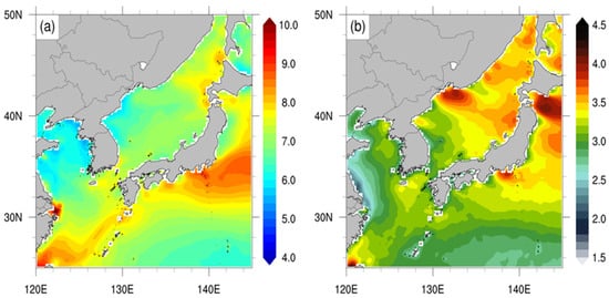
Figure 2.
Spatial distribution of (a) annual mean wind speeds (m·s−1) and (b) wind speed variability (m·s−1) (standard deviation) based on DASCAT during 2008–2017.
Since DASCAT only provided daily wind speed data, the time scale of the observation data was scaled up for comparison. DASCAT data were extracted from the closest grids to the location of observation buoys. Buoy wind speeds for each location—YS (DJ, CB, and OY), KS (GM, GJ, MR, and SG), and ES (DH, PH, UL, UJ, and US)—were compared with DASCAT estimates (Figure 3) and detailed statistics are shown in Table 3. The quantile distributions showed deviations for the extremes and also DASCAT data had a positive bias at all buoy stations. Since DASCAT was derived from ASCAT level 2b with auxiliary ECMWF analysis data, scatterometer data from some YS and some KS locations are missing. ES buoy locations had a relatively lower bias, RMSE, and higher correlation coefficients than those in the YS and KS. The positive bias of DASCAT estimates increased with buoy wind speeds. These results were similar to those found previously [55], as well as to those from the YS and Bohai Sea [22].
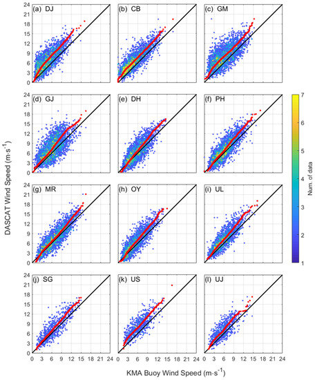
Figure 3.
Scatter and quantile–quantile plots of daily wind speed (red dots) between in situ buoy Scheme 2008 (a–l). Colors indicates the density of data in each 50 × 50 bin. Panels are ordered according to observation starting dates.
Table 3.
Error metrics for the daily wind speeds derived from buoy observation stations (OBS) and DASCAT.
An hourly comparison of the WRF hindcast values was conducted against buoy observations (Figure 4) and detailed error metrics are described in Table 4. Correlation coefficients >0.6 were recorded across all stations, with a slight positive bias in quantiles with speeds >10 m·s−1. Moreover, the quantiles displayed nearly identical distribution. The RMSE was <2.5 m·s−1, except at GM and GJ. The positive bias was <1 m·s−1, except at MR and CB. The WRF hindcast wind speeds tended to be overestimated at wind speeds >10 m·s−1. Although DASCAT data were inconsistent with buoy data across analyzed points, the WRF hindcast showed consistency.
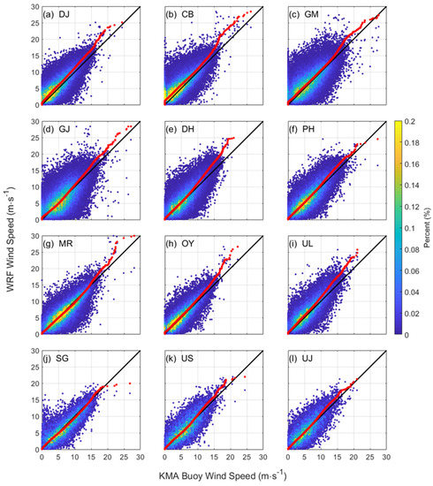
Figure 4.
Scatter and quantile–quantile plots of hourly wind speed between in situ observations (x-axis) and WRF hindcast data (y-axis) during 1997–2017 (a–l). Colors indicate the percentage of data in each 100 × 100 bin and red dots represent the percentile values of the quantile–quantile plots.
Table 4.
Error metrics for the wind speed derived from buoy observation stations (OBS) and the Weather Research and Forecasting (WRF) model hindcast.
3.2. Added Value Evaluation
The WRF hindcast data were obtained through dynamic downscaling. It was assumed that the regional model could have added value compared to the ERA-Interim global model and simulations around the KP were evaluated using the modified BSS defined in Section 2.5 (Figure 5). Assuming DASCAT data as “True,” the spatial and temporal domain of ERA-Interim and hindcast data were interpolated and compared. Offshore wind speeds in the ECS, west of the YS, and in the far seas of the ES had negative BSS values, indicating no added value from the hindcast data. Positive BSS values appeared along the coastal areas, supporting the use of the added hindcast data. In the coastal areas of the KS, Japan, and the southern region of the ES, hindcast data displayed an added value. Wind characteristics originating from the land, sea breeze circulation, or topographical factors mostly occur near coastal areas rather than offshore; therefore, the added value of the WRF hindcast data may depend on such wind features. These results are similar to those of previous studies in the Mediterranean and Western European regions [21], the YS, and the Bohai Sea [22].
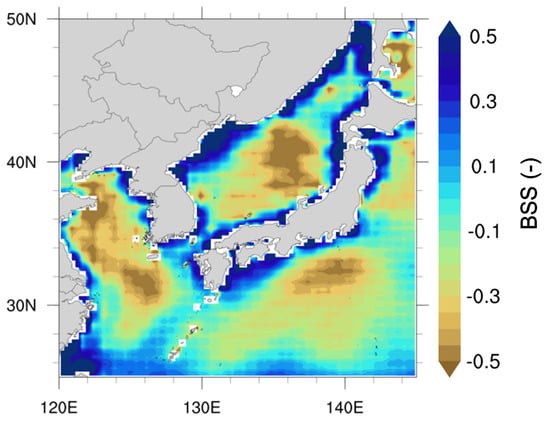
Figure 5.
Modified Brier skill score (BSS) spatial distribution of wind speed error variance comparing hindcast estimates against ERA-Interim data, where DASCAT values were regarded as “True”.
3.2.1. Seasonality of the Added Value
As East Asia has a monsoonal climate, seasonality accounts for a large proportion of wind speed variability. In order to investigate the seasonal added value of hindcast data, the data were divided into spring (MAM), summer (JJA), autumn (SON), and winter (DJF) and the BSS was calculated following the same methods (Figure 6). The correlation between DASCAT and hindcast data tended to be higher in the YS and offshore of the ES in the autumn and winter than in spring and summer (Figure 6a–d). Data in the YS and ECS had a higher correlation (>0.85) than that in the Bohai Sea, northeastern part of the ES, and coastal region of Japan (<0.6). Along the KP coast, the correlation was lower than that offshore across all seasons. Moreover, the correlations were lower in the spring and summer than in the autumn and winter. The hindcast data underestimated the wind speeds in all seasons near the coast of the KP (Figure 6e–f).
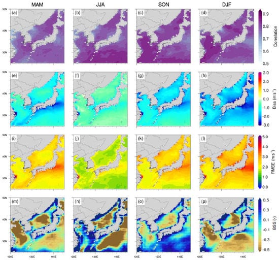
Figure 6.
Spatial distribution of the following: (a–d) correlation, (e–h) bias, (i–l) RMSE, and (m–p) modified BSS throughout the four seasons, where MAM, JJA, SON, and DJF indicate spring, summer, autumn, and winter, respectively.
Regionally, WRF underestimated wind speeds by up to 2 m·s−1 in the Bohai Sea from autumn to winter and along the ES coast during the winter. The open sea area had a negative bias of >1 m·s−1 across all seasons except the summer and the coast of the ECS showed a negative bias of >3 m·s−1 for all seasons. Whereas the WRF hindcast data had a negative bias, DASCAT showed a positive bias when compared to the buoy observation (Figure 3, Table 3) and was thus deemed acceptable. In Figure 6i–l, YS had a slightly lower seasonal variability of RMSE than other areas and its overall value was relatively low. The RMSE of the coastal areas of KP was higher than that of the open sea, regardless of the season, and never exceeded 3 m·s−1. As shown in Figure 6m–p, the most significant differences in BSS were between summer and winter. YS, the Bohai Sea, and most of the KS showed a strongly positive BSS in the summer and a negative BSS in the spring, autumn, and winter, except for coastal KP. The added value of the WRF hindcast data was well represented along the entire KP coast, across all seasons (except for the northeastern ES during spring and summer). This means that the WRF hindcast data around the coast of the KP reproduced sea surface wind speeds better than ERA-Interim.
3.2.2. Added Value in Wind Intensities
It has been well-established in the literature that DASCAT wind speed data are significantly correlated within the range of 3–25 m·s−1 [23]; therefore, it was divided into weak (3–5 m·s−1), moderate (5–10 m·s−1), and strong wind speeds (10–25 m·s−1) for added value comparison. In the WRF hindcast data for the coastal area of the KP, >60% of all wind speeds were weak or moderate and <20% were strong (Figure 7a–c). Regionally, KS appeared to experience more moderate and strong wind speeds compared to ES and YS.
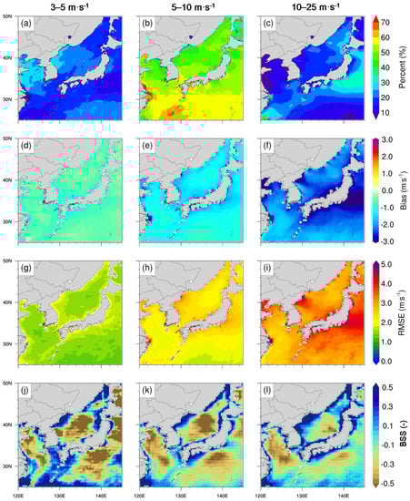
Figure 7.
Spatial distributions of different wind intensities: 3–5 m·s−1 (a,d,g,j); 5–10 m·s−1 (b,e,h,k); and 10–25 m·s−1 (c,f,i,l). (a–c) displays the percentage of each wind intensity within the valid range of DASCAT (3–25 m·s−1), (d–f) shows the mean bias of hindcast and DASCAT data, (g–i) displays the RMSE of hindcast and DASCAT data, and (j–l) display the BSS of the hindcast relative to ERA-Interim when DASCAT is considered as “True”.
The bias of the KP coast is approximately −1 for weak, −1 to −2 for moderate, and −2 to −3 for strong wind speeds. Thus, as the wind speed increased, a stronger negative bias appeared (Figure 7d–f). The RMSE around KP showed a lower value for strong wind speeds than for weak and moderate wind speeds (Figure 7g–i). The coastal areas of the KP showed a slightly higher RMSE than open sea areas across all wind speeds analyzed. Most notably, WRF hindcasts added the predictive value in the coastal areas of YS and KS, regardless of wind speed (Figure 7j–l). Although the ES coast did not express an obvious added value under weak and moderate wind speeds, a high added value was observed under strong wind speeds. Moreover, a significant added value under strong wind conditions was noticed for a considerable range of open sea areas of the ES. Overall, WRF hindcast data in coastal regions of KP added value across all wind intensities analyzed, which was especially true under strong wind conditions, indicating a more accurate simulation than ERA-Interim alone across the coastal regions under the influence of regional-scale circulation and topographical effects.
3.3. Estimation of Extreme Wind Speeds
To estimate extreme wind speeds, it is necessary to evaluate the extreme value distribution of the time-series data. To this end, empirical studies have demonstrated that wind speed can be statistically evaluated to follow the characteristics of the two-parameter Weibull distribution [21,59,60,61], where the probability distribution function (PDF) of the random variable is defined according to Equation (2):
where is the scale parameter related to the mean wind speed and is the shape parameter representing the magnitude of the deviation of the wind speed. There are numerous mathematical methods to calculate the scale and shape parameters, such as the method of momentum (MOM), maximum likelihood estimator (MLE), and L-moment. In general, MOM is employed when population and sample sizes match, MLE is used when estimating parameters from an assumed distribution pattern, and the L-moment is useful when the sample size is small. Accordingly, MLE was adopted for parameter estimation, where the wind speed followed a two-parameter Weibull distribution at confidence intervals of 95%.
Maximum daily wind speed was extracted from the WRF hindcast data and parameter estimation was performed with MLE. Figure 8 shows the spatial distribution of the shape and scale parameters of the Weibull distribution from the WRF hindcast data. The shape parameters were ~2.6–2.9 for the YS, ~2.9 for KS, and ~2.8 for ES. In particular, the shape parameters on the coast of KS, ES, Bohai Sea, and Chinese coasts were >3.0. The scale parameters were ~9–10 for the YS, ~10–10.5 for KS, and >10.4 for ES. The scale parameter of the Bohai Sea was >10 and that of the Chinese coastal waters was <8.6.
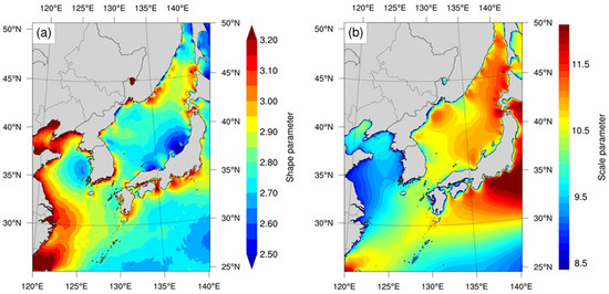
Figure 8.
Spatial distribution of the (a) shape and (b) scale parameter of the Weibull distribution from the daily maximum WRF hindcast wind speed data (1979–2017).
Through the scale and shape parameters, it was possible to understand the spatial characteristics of wind speed distribution around the KP. Steady winds with weak variability were the reason for the lower shape parameter recorded in YS than in the ES or KS. Alternatively, regional differences in climatic land–sea breeze circulation may have been caused by higher shape parameters along the coast of the ES and KS. The scale parameters of the ES were the highest (≥10.2), and those of the YS were the lowest (≤9.4), indicating that the annual mean wind speed was of the same order. The spatial distribution of the Weibull parameters showed a significant difference in the climatic characteristics of the sea surface wind distribution across the KP; however, the physical and dynamic processes that resulted in these statistical results require further research.
Extreme wind speed estimates are a critical external force condition to consider for designs that consider wind resistance and for structural safety evaluations of offshore structures [61]. Although long-term observation data are unequivocal for extreme wind speed estimation, it is difficult to obtain reliable and continuous long-term oceanic observation data. Individual observations by marine meteorological buoys are often missing due to weather conditions, thus inhibiting accurate estimates of extreme values. In addition, because data are acquired in the form of observation point data, it is difficult to estimate the spatial distribution of extreme values. To overcome this limitation, prior studies obtained long-term reanalysis or hindcast data through numerical simulations to calculate extreme wind speeds [21]. For a given return period (typically 50 or 100 years), the extreme wind speeds can be estimated based on the parameters of the Weibull distribution. Therefore, 50-year and 100-year return period wind speeds were estimated in the present study following the quantile function of the Weibull distribution according to Equation (3) as described as follows:
where is the probability of the return period derived from , for which is the annual time interval of the data and is the return period. The spatial variabilities of the wind speed for 50-year and 100-year return periods were similar (Figure 9). The 100 year return period wind speed was ~18–20 m·s−1 YS, ~22–23 m·s−1 for the KS, and >23 m·s−1 for the ES. The occurrence of extreme wind speeds in the Bohai Sea and along the coast of China was relatively rarer than around the KP. The spatial distribution of the Weibull parameters and the extreme wind speed along the ES coast had different characteristics because of the montane topographic effects and sea–land breeze circulations. The results of extreme wind speeds can be used by practitioners as a reference for evaluating the stability of structures (e.g., wind turbines) along the KP.
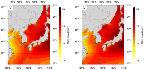
Figure 9.
Distributions of estimated (a) 50-year and (b) 100-year return period wind speeds (m·s−1).
4. Discussion
In this study, 39 years of historical data for all sea areas surrounding the KP were produced and validated for sea surface winds using ERA-Interim for initial and boundary conditions. Sensitivity experiments were performed for the PBL scheme, crucial for developing sea surface wind hindcasts. The YSU PBL scheme was selected for obtaining the same results as in previous studies [21,38]. Implementation of 3DVAR data assimilation was performed and the WRF hindcast data were produced by combining daily simulations. To verify hindcasts, DASCAT data were adopted which were generated based on the ASCAT-L2 satellite data. DASCAT data was then compared with KMA buoy data observed across the KP coasts from 1997–2017 to support using spatially uniform gridded DASCAT data as “True.” This assumption may cause uncertainty in WRF hindcast evaluation. The uncertainty may change depending on which data were referred as “True.” However, there are not many spatiotemporally consistent data in the seas around the KP. Since the previous study presented high accuracy of DASCAT in comparison with other reanalysis data [24], satellite-based DASCAT data were referred as “True” in this study. In addition, the KMA buoy data was used as reference in situ data because it can cover the most extended period. However, most of all, in order to verify the accuracy of RCM simulation with respect to considering the observation uncertainty, it is essential to improve the quality of observation data.
Regardless of the area analyzed, a positive bias with a value of <2 m·s−1 were observed. A further comparison against KMA buoy data was carried out to evaluate the reliability of the WRF hindcast data and the bias of all buoy stations (except CB) was <1 m·s−1. Moreover, the RMSE was <2.5 m·s−1 for all buoy stations, except GM and GJ. Overall, the statistics showed good agreement between in situ observations and WRF hindcast data. A modified BSS was used to evaluate the added value of the WRF hindcast data obtained via the dynamic downscaling of ERA-Interim. Over the entire period (2008–2017), the added value of the hindcast primarily manifested in the coastal regions. The added value was also analyzed in terms of seasonal variability and wind speed; as the variability of wind speeds for each season in East Asia are different owing to the monsoonal climate, it was assumed that the added value would also vary seasonally. The added value manifested along the coast of the YS during the summer and along the coast of the ES during the winter, while it manifested regardless of the season in the coastal area of the KS. As for the added value with respect to wind speed, stronger winds resulted in a lower RMSE. An added value was observed along the coast of the KP under strong wind conditions, revealing a different result from that in previous research [22] where sea surface winds of the KP coast could have resulted in an added value owing to the high spatiotemporal resolution and data assimilation. The presence of this added value indicated adequate reproduction of the large-scale atmospheric circulation of westerly and monsoonal climates.
The negative BSS appears in the offshore and open sea areas of ES and YS in all wind speeds and seasons. These results are consistent with the previous studies [20,22] and it has been expressed that there is no added value of RCM simulation in offshore and open sea area. Nevertheless, the accuracy of the WRF hindcast can be evaluated relatively low because DASCAT data filled with ERA-Interim where there was no direct satellite observation. In addition, it seems that the wind speed in the open sea areas is determined by global-scale circulation and dynamics. Further study is needed for precise analysis.
This study provided long-term and homogeneous sea–surface wind data for the seas around the KP and the added value was the greatest in the coastal areas rather than in open sea areas. These results are corroborated by previous research in other regions [20,22]. In detail, comparison results show the improvement of this study from the lowest RMSE buoy points compared with hindcast. At OY station in YS, Heo and Ha [5] showed RMSE of 1.83 m·s−1, a bias of 0.59 m·s−1, and correlation of 0.86 samples using FNL as initial and boundary conditions. Heo et al. [39] assessed RMSE of 2.08 m·s−1, bias of 0.40, and correlation of 0.87 using ERA-Interim as initial and boundary conditions. Both studies only used one year (2014) hindcast data with 8426 samples. In this study, RMSE of 1.80 m·s−1, bias of 0.41 m·s−1, and correlation of 0.84 were obtained from 65320 samples from October 2008. Considering that buoy observation compared from the start date, these results show the improvement of this study well.
The WRF hindcast showed reliable accuracy regardless of season and wind speed. However, the wind direction was not considered because this study focused on the statistical characteristics of long-term hindcast data. For the analysis of wind direction, dynamics must be considered. The physical and dynamic processes that result in the added value of the developed model were not investigated. Accordingly, synoptic processes that are known factors that affect local wind climates, such as sea and land breeze circulation, were not investigated [62]. Additionally, tropical cyclones (TCs) strongly affect the weather system around KP. Although TCs may be correlated with the added value of strong wind conditions revealed here, detailed processes were not considered. Added value was primarily assessed using statistical analyses and further studies will be required to investigate the underlying dynamic processes.
The extreme wind speed estimates were based on the well-established credibility of the WRF hindcast data with a high spatiotemporal resolution. The climatological and statistical characteristics of wind speed over the entire study period were expressed using a Weibull distribution. On the coast of the KP, the shape parameter was 2.75–3.1 and the scale showed a distribution similar to that of the climatology. The return period wind speed along the coast of the KP was ~20 m·s−1 in YS and KS and ~23 m·s−1 in ES.
5. Summary and Conclusions
This study provided long-term and high spatiotemporal resolution sea surface wind hindcast data for the seas around the KP. A summary of the key findings from this study is as follows:
- A long-term hindcast data produced by state of the art WRF model using ERA-Interim as initial and boundary conditions. Adoption of 3DVAR data assimilation was conducted for a 39 year (1979–2017) simulation to make accurate initial conditions.
- By comparison with KMA buoy data, DASCAT was employed and regarded as “True”. The WRF hindcast was also compared with the buoy data for reliability and it showed high accuracy.
- The added value was evaluated using modified BSS and analyzed for seasonality and wind intensity. The WRF hindcast adds value to the coastal areas of KP, particularly over YS in the summer, ES in the winter, and KS in all seasons. In the case of strong winds, the hindcast performed better in the coastal areas of KP.
- The extreme wind speed estimates were performed by using the parameters of the Weibull distribution for the 50 year and 100 year return period based on the produced hindcast data on the climate scale.
The long-term WRF hindcast data can provide useful information for maritime activities, shipping routes, structural safety evaluations, etc. In addition, these results can serve as a reference dataset for climate perspective storm surge and wave simulation studies.
Supplementary Materials
The following are available online at https://www.mdpi.com/article/10.3390/atmos12070895/s1, Table S1: Physics and parameterization scheme configuration of sensitivity test, Figure S1: Taylor diagram for the wind speed over study area from 8 sensitivity test simulations for ERA-Interim and NCEP FNL, Figure S2: Time series of model wind speed at each buoy station, Figure S3: Scatter plots of hourly wind speed between buoy observations and model wind speed, Table S2: Error metrics for the hourly wind speed derived from buoy observations and each sensitivity test.
Author Contributions
Conceptualization, H.K., K.-Y.H. and J.-I.K.; methodology, H.K. and N.-H.K.; formal analysis, H.K.; investigation, H.K.; data curation, H.K. and K.-Y.H.; visualization, H.K.; writing—original draft preparation, H.K., N.-H.K. and K.-Y.H.; writing—review and editing, H.K. and K.-Y.H.; supervision, J.-I.K.; funding acquisition, J.-I.K. All authors have read and agreed to the published version of the manuscript.
Funding
This research was part of the project titled “Improvements of ocean prediction accuracy using numerical modeling and artificial intelligence technology (PM62220)” funded by the Ministry of Oceans and Fisheries, Korea. This work was also supported by KIOST (Grant PE99942).
Data Availability Statement
ERA-Interim data are at https://www.ecmwf.int/en/forecasts/datasets/reanalysis-datasets/era-interim (accessed on 17 May 2021), KMA buoy data are at https://data.kma.go.kr (accessed on 17 May 2021), and DASCAT data are at http://apdrc.soest.hawaii.edu (accessed on 17 May 2021), respectively.
Acknowledgments
We thank the Korea Meteorological Administration and the European Center for Medium-Range Weather Forecasts for the datasets used. We would also like to thank the three reviewers for their invaluable suggestions and comments.
Conflicts of Interest
The authors declare no conflict of interest.
References
- Powell, M.D.; Murillo, S.; Dodge, P.; Uhlhorn, E.; Gamache, J.; Cardone, V.; Cox, A.; Otero, S.; Carrasco, N.; Annane, B.; et al. Reconstruction of Hurricane Katrina’s wind fields for storm surge and wave hindcasting. Ocean Eng. 2010, 37, 26–36. [Google Scholar] [CrossRef]
- Weisse, R.; von Storch, H.; Niemeyer, H.D.; Knaack, H. Changing North Sea storm surge climate: An increasing hazard? Ocean Coast. Manag. 2012, 68, 58–68. [Google Scholar] [CrossRef]
- Lee, S.H.; Kim, D.H.; Lee, H.W. Satellite-based assessment of the impact of sea-surface winds on regional atmospheric circulations over the Korean Peninsula. Int. J. Remote Sens. 2008, 29, 331–354. [Google Scholar] [CrossRef]
- Kim, J.-Y.; Oh, K.-Y.; Kang, K.-S.; Lee, J.-S. Site selection of offshore wind farms around the Korean Peninsula through economic evaluation. Renew. Energy 2013, 54, 189–195. [Google Scholar] [CrossRef]
- Heo, K.-Y.; Ha, T. Producing the hindcast of wind and waves using a high-resolution atmospheric reanalysis around Korea. J. Coast. Res. 2016, 75, 1107–1111. [Google Scholar] [CrossRef]
- Lee, D.-Y.; Jun, K.-C. Estimation of Design Wave Height for the Waters around the Korean Peninsula. Ocean Sci. J. 2006, 41, 245–254. [Google Scholar] [CrossRef]
- Kim, G.-U.; Seo, K.-H.; Chen, D. Climate change over the Mediterranean and current destruction of marine ecosystem. Sci. Rep. 2019, 9, 1–9. [Google Scholar] [CrossRef] [PubMed]
- Son, J.-H.; Seo, K.-H.; Wang, B. How Does the Tibetan Plateau Dynamically Affect Downstream Monsoon Precipitation? Geophys. Res. Lett. 2020, 47, 090543. [Google Scholar] [CrossRef]
- Son, J.-H.; Seo, K.-H.; Son, S.-W.; Cha, D.-H. How Does Indian Monsoon Regulate the Northern Hemisphere Stationary Wave Pattern? Front. Earth Sci. 2021, 8, 587. [Google Scholar] [CrossRef]
- Brands, S.; Gutiérrez, J.M.; Herrera, S.; Cofiño, A. On the use of reanalysis data for downscaling. J. Clim. 2012, 25, 2517–2526. [Google Scholar] [CrossRef][Green Version]
- Dee, D.P.; Uppala, S.M.; Simmons, A.J.; Berrisford, P.; Poli, P.; Kobayashi, S.; Andrae, U.; Balmaseda, M.A.; Balsamo, G.; Bauer, P.; et al. The ERA-Interim reanalysis: Configuration and performance of the data assimilation system. Q. J. R. Meteorol. Soc. 2011, 137, 553–597. [Google Scholar] [CrossRef]
- Feser, F.; Rockel, B.; von Storch, H.; Winterfeldt, J.; Zahn, M. Regional Climate Models Add Value to Global Model Data: A Review and Selected Examples. Bull. Am. Meteorol. Soc. 2011, 92, 1181–1192. [Google Scholar] [CrossRef]
- Li, D. Added value of high-resolution regional climate model: Selected cases over the Bohai Sea and the Yellow Sea areas. Int. J. Climatol. 2016, 37, 169–179. [Google Scholar] [CrossRef]
- Manzanas, R.; Gutiérrez, J.M.; Fernández, J.; Van Meijgaard, E.; Calmanti, S.; Magariño, M.E.; Cofiño, A.S.; Herrera, S. Dynamical and statistical downscaling of seasonal temperature forecasts in Europe: Added value for user applications. Clim. Serv. 2018, 9, 44–56. [Google Scholar] [CrossRef]
- Kelemen, F.D.; Primo, C.; Feldmann, H.; Ahrens, B. Added Value of Atmosphere-Ocean Coupling in a Century-Long Regional Climate Simulation. Atmosphere 2019, 10, 537. [Google Scholar] [CrossRef]
- Qiu, L.; Im, E.-S.; Hur, J.; Shim, K.-M. Added value of very high resolution climate simulations over South Korea using WRF modeling system. Clim. Dyn. 2019, 54, 173–189. [Google Scholar] [CrossRef]
- Di Virgilio, G.; Evans, J.P.; Di Luca, A.; Grose, M.R.; Round, V.; Thatcher, M. Realised added value in dynamical downscaling of Australian climate change. Clim. Dyn. 2020, 54, 4675–4692. [Google Scholar] [CrossRef]
- Politi, N.; Vlachogiannis, D.; Sfetsos, A.; Nastos, P.T. High-resolution dynamical downscaling of ERA-Interim temperature and precipitation using WRF model for Greece. Clim. Dyn. 2021, 1–27. [Google Scholar] [CrossRef]
- Ebuchi, N.; Graber, H.C.; Caruso, M.J. Evaluation of Wind Vectors Observed by QuikSCAT/SeaWinds Using Ocean Buoy Data. J. Atmos. Ocean Technol. 2002, 19, 2049–2062. [Google Scholar] [CrossRef]
- Winterfeldt, J.; Geyer, B.; Weisse, R. Using QuikSCAT in the added value assessment of dynamically downscaled wind speed. Int. J. Climatol. 2010, 31, 1028–1039. [Google Scholar] [CrossRef]
- Menendez, M.; García-Díez, M.; Fita, L.; Fernández, J.; Mendez, F.; Gutiérrez, J.M. High-resolution sea wind hindcasts over the Mediterranean area. Clim. Dyn. 2013, 42, 1857–1872. [Google Scholar] [CrossRef]
- Li, D.; Von Storch, H.; Geyer, B. High-resolution wind hindcast over the Bohai Sea and the Yellow Sea in East Asia: Evaluation and wind climatology analysis. J. Geophys. Res. Atmos. 2016, 121, 111–129. [Google Scholar] [CrossRef]
- Sivareddy, S.; Ravichandran, M.; GirishKumar, M.S. Evaluation of ASCAT-Based Daily Gridded Winds in the Tropical Indian Ocean. J. Atmos. Ocean Technol. 2013, 30, 1371–1381. [Google Scholar] [CrossRef]
- Park, J.; Kim, D.-W.; Jo, Y.-H.; Kim, D. Accuracy evaluation of daily-gridded ASCAT satellite data around the Korean Pen-insula. Korean J. Remote Sens. 2018, 34, 213–225. [Google Scholar] [CrossRef]
- Na, J.-Y.; Seo, J.-W.; Han, S.-K. Monthly-mean sea surface winds over the adjacent seas of the Korea Peninsular. J. Ocean Soc. Korean 1992, 27, 1–10. [Google Scholar]
- Lee, D.-K.; Kwon, J.-I.; Hahn, S.-B. The wind effect on the cold water formation near Gampo-Ulgi coast. Korean J. Fish. Aq. Sci. 1998, 31, 359–371. [Google Scholar]
- Seo, J.-W.; Chang, Y.-S. Characteristics of the monthly mean sea surface winds and wind waves near the Korean marginal seas in 2002 Computed Using MM5/KMA and WAVEWATCH-III model. Sea J. Korean Soc. Ocean 2003, 8, 262–273. [Google Scholar]
- Kim, Y.-K.; Jeong, J.-H.; Bae, J.-H.; Oh, I.-B.; Kweon, J.-H.; Seo, J.-W. Improvement in the simulation of sea surface wind over the complex coastal area using WRF model. J. Korean Soc. Atmo. Environ. 2006, 22, 309–323. [Google Scholar]
- Yoon, H.-J.; Park, K.-S.; Kim, S.-I. Ocean wind retrieval from RADAR SAR images in Korean seas. J. Korean Inst. Inf. Commun. Eng. 2006, 10, 706–711. [Google Scholar]
- You, S.H.; Cho, J.-G.; Seo, J.-W. Comparison of KMA operational model RDAPS with QuikSCAT sea surface wind data. J. Korean Soc. Coast. Oceanogr. Eng. 2007, 19, 467–475. [Google Scholar]
- Jeong, J.-Y.; Shim, J.-S.; Lee, D.-K.; Min, I.-K.; Kwon, J.-I. Validation of QuikSCAT Wind with Resolution of 12.5 km in the Vicinity of Korean Peninsula. Ocean Polar Res. 2008, 30, 47–58. [Google Scholar] [CrossRef][Green Version]
- Heo, K.-Y.; Lee, J.-W.; Ha, K.-J.; Jun, K.-C.; Park, K.-S. Model Optimization for Sea Surface Wind Simulation of Strong Wind Cases. J. Korean Earth Sci. Soc. 2008, 29, 263–279. [Google Scholar] [CrossRef][Green Version]
- Lee, S.-H.; Lee, H.-W.; Kim, D.-H.; Kim, M.-J.; Kim, H.-G. Numerical Study on the Impact of the Spatial Resolution of Wind Map in the Korean Peninsula on the Accuracy of Wind Energy Resources Estimation. J. Environ. Sci. Int. 2009, 18, 885–897. [Google Scholar] [CrossRef]
- Li, D.; Geyer, B.; Bisling, P. A model-based climatology analysis of wind power resources at 100-m height over the Bohai Sea and the Yellow Sea. Appl. Energy 2016, 179, 575–589. [Google Scholar] [CrossRef]
- Choi, W.; Shin, H.-J.; Jang, C.J. Evaluation of climatological mean surface winds over Korean waters simulated by CORDEX-EA regional climate models. Atmos. Korean Met. Soc. 2019, 29, 115–129. [Google Scholar] [CrossRef]
- Yu, Y.; Zhang, W.; Wu, Z.; Yang, X.; Cao, X.; Zhu, M. Assimilation of HY-2A scatterometer sea surface wind data in a 3DVAR data assimilation system—A case study of Typhoon Bolaven. Front. Earth Sci. 2015, 9, 192–201. [Google Scholar] [CrossRef]
- Yu, Y.; Yang, X.; Zhang, W.; Duan, B.; Cao, X.; Leng, H. Assimilation of Sentinel-1 derived sea surface winds for typhoon forecasting. Remote Sens. 2017, 9, 845. [Google Scholar] [CrossRef]
- Kwun, J.H.; Kim, Y.-K.; Seo, J.-W.; Jeong, J.H.; You, S.H. Sensitivity of MM5 and WRF mesoscale model predictions of surface winds in a typhoon to planetary boundary layer parameterizations. Nat. Hazards 2009, 51, 63–77. [Google Scholar] [CrossRef]
- Heo, K.-Y.; Ha, T.; Choi, J.-Y.; Park, K.-S.; Kwon, J.-I.; Jun, K. Evaluation of Wind and Wave Simulations using Different Global Reanalyses. J. Coast. Res. 2017, 79, 99–103. [Google Scholar] [CrossRef]
- Byun, D.-S.; Choi, B.-J. Nomenclature of the seas around the Korean Peninsula derived from analyses of papers in two repre-sentative Korean ocean and fisheries Science Journals: Present Status and Future. Sea J. Korean Soc. Oceanogr. 2018, 23, 125–151. [Google Scholar] [CrossRef]
- Skamarock, W.C.; Klemp, J.B.; Dudhia, J.; Gill, D.O.; Barker, D.M.; Wang, W.; Powers, J.G. A Description of the Advanced Research WRF Version 3. NCAR Technical Note-475+ STR. 2008. Available online: https://opensky.ucar.edu/islandora/object/technotes%3A500/datastream/PDF/view (accessed on 9 July 2021).
- Hahmann, A.N.; Vincent, C.; Peña, A.; Lange, J.; Hasager, C.B. Wind climate estimation using WRF model output: Method and model sensitivities over the sea. Int. J. Climatol. 2015, 35, 3422–3439. [Google Scholar] [CrossRef]
- Kim, Y.-K.; Jeong, J.-H.; Bae, J.-H.; Song, S.-K.; Seo, J.-W. Study on planetary boundary layer schemes suitable for simulation of sea surface wind in the southeastern coastal area, Korea. J. Environ. Sci. Int. 2005, 14, 1015–1026. [Google Scholar] [CrossRef]
- Carvalho, D.; Rocha, A.; Gómez-Gesteira, M.; Santos, C.S. Sensitivity of the WRF model wind simulation and wind energy production estimates to planetary boundary layer parameterizations for onshore and offshore areas in the Iberian Peninsula. Appl. Energy 2014, 135, 234–246. [Google Scholar] [CrossRef]
- Hong, S.-Y.; Noh, Y.; Dudhia, J. A New Vertical Diffusion Package with an Explicit Treatment of Entrainment Processes. Mon. Weather Rev. 2006, 134, 2318–2341. [Google Scholar] [CrossRef]
- Hong, S.-Y.; Lim, J.-O.J. The WRF single-moment 6-class microphysics scheme (WSM6). Asia-Pac. J. Atmo. Sci. 2006, 42, 129–151. [Google Scholar]
- Dudhia, J. Numerical study of convection observed during the winter monsoon experiment using a mesoscale two-dimensional model. J. Atmo. Sci. 1989, 46, 3077–3107. [Google Scholar] [CrossRef]
- Kain, J.S.; Fritsch, J.M. Convective Parameterization for Mesoscale Models: The Kain-Fritsch Scheme. In The Representation of Cumulus Convection in Numerical Models; Emanuel, K.A., Raymond, D.J., Eds.; American Meteorological Society: Boston, MA, USA, 1993; Volume 46, pp. 165–170. [Google Scholar]
- Niu, G.-Y.; Yang, Z.-L.; Mitchell, K.E.; Chen, F.; Ek, M.B.; Barlage, M.; Kumar, A.; Manning, K.; Niyogi, D.; Rosero, E.; et al. The community Noah land surface model with multiparameterization options (Noah-MP): 1. Model description and evaluation with local-scale measurements. J. Geophys. Res. Space Phys. 2011, 116. [Google Scholar] [CrossRef]
- Chu, Q.; Xu, Z.; Chen, Y.; Han, D. Evaluation of the ability of the Weather Research and Forecasting model to reproduce a sub-daily extreme rainfall event in Beijing, China using different domain configurations and spin-up times. Hydrol. Earth Syst. Sci. 2018, 22, 3391–3407. [Google Scholar] [CrossRef]
- Liu, J.; Wang, J.; Pan, S.; Tang, K.; Li, C.; Han, D. A real-time flood forecasting system with dual updating of the NWP rainfall and the river flow. Nat. Hazards 2015, 77, 1161–1182. [Google Scholar] [CrossRef]
- Carlin, J.T.; Gao, J.; Snyder, J.C.; Ryzhkov, A.V. Assimilation of ZDR Columns for Improving the Spinup and Forecast of Convective Storms in Storm-Scale Models: Proof-of-Concept Experiments. Mon. Weather Rev. 2017, 145, 5033–5057. [Google Scholar] [CrossRef]
- Li, D.; Von Storch, H.; Geyer, B. Testing Reanalyses in Constraining Dynamical Downscaling. J. Meteorol. Soc. Jpn. 2016, 94A, 47–68. [Google Scholar] [CrossRef]
- Queffeulou, P.; Chapron, B.; Bentamy, A. Comparing Ku-band NSCAT scatterometer and ERS-2 altimeter winds. IEEE Trans. Geosci. Remote Sens. 1999, 37, 1662–1670. [Google Scholar] [CrossRef]
- Bentamy, A.; Fillon, D.C. Gridded surface wind fields from Metop/ASCAT measurements. Int. J. Remote Sens. 2011, 33, 1729–1754. [Google Scholar] [CrossRef]
- Von Storch, H. Misuses of statistical analysis in climate research. In Analysis of Climate Variability; Springer: Berlin/Heidelberg, Germany, 1999; pp. 11–26. [Google Scholar]
- Geyer, B.; Weisse, R.; Bisling, P.; Winterfeldt, J. Climatology of North Sea wind energy derived from a model hindcast for 1958–2012. J. Wind. Eng. Ind. Aerodyn. 2015, 147, 18–29. [Google Scholar] [CrossRef]
- Kumar, D.; Dimri, A.P. Context of the added value in coupled atmosphere-land RegCM4–CLM4.5 in the simulation of Indian summer monsoon. Clim. Dyn. 2021, 56, 259–274. [Google Scholar] [CrossRef]
- Pavia, E.G.; O’Brien, J.J. Weibull Statistics of Wind Speed over the Ocean. J. Clim. Appl. Meteorol. 1986, 25, 1324–1332. [Google Scholar] [CrossRef]
- Seguro, J.; Lambert, T. Modern estimation of the parameters of the Weibull wind speed distribution for wind energy analysis. J. Wind Eng. Ind. Aerodyn. 2000, 85, 75–84. [Google Scholar] [CrossRef]
- Monahan, A.H. The Probability Distribution of Sea Surface Wind Speeds. Part I: Theory and SeaWinds Observations. J. Clim. 2006, 19, 497–520. [Google Scholar] [CrossRef]
- Masselink, G.; Pattiaratchi, C. Characteristics of the sea breeze system in Perth, Western Australia, and its effect on the near-shore wave climate. J. Coast. Res. 2001, 17, 173–187. [Google Scholar]


Publisher’s Note: MDPI stays neutral with regard to jurisdictional claims in published maps and institutional affiliations. |
© 2021 by the authors. Licensee MDPI, Basel, Switzerland. This article is an open access article distributed under the terms and conditions of the Creative Commons Attribution (CC BY) license (https://creativecommons.org/licenses/by/4.0/).