Review of Long-Term Trends in the Equatorial Ionosphere Due the Geomagnetic Field Secular Variations and Its Relevance to Space Weather

Abstract

The Earth’s ionosphere presents long-term trends that have been of interest since a pioneering study in 1989 suggesting that greenhouse gases increasing due to anthropogenic activity will produce not only a troposphere global warming, but a cooling in the upper atmosphere as well. Since then, long-term changes in the upper atmosphere, and particularly in the ionosphere, have become a significant topic in global change studies with many results already published. There are also other ionospheric long-term change forcings of natural origin, such as the Earth’s magnetic field secular variation with very special characteristics at equatorial and low latitudes. The ionosphere, as a part of the space weather environment, plays a crucial role to the point that it could certainly be said that space weather cannot be understood without reference to it. In this work, theoretical and experimental results on equatorial and low-latitude ionospheric trends linked to the geomagnetic field secular variation are reviewed and analyzed. Controversies and gaps in existing knowledge are identified together with important areas for future study. These trends, although weak when compared to other ionospheric variations, are steady and may become significant in the future and important even now for long-term space weather forecasts.

1. Introduction

The Earth’s ionosphere at low latitudes depends strongly on solar radiation, the geomagnetic field, and atmospheric conditions [1], all of which present variabilities in different time scales. In addition to regular changes such as daily and seasonal, and irregular variations of transient character, this upper atmosphere region presents long-term trends as well. They have been of interest since a pioneering study in 1989 suggesting that the long-term increase of greenhouse gases concentration due to anthropogenic activity, particularly carbon dioxide (CO₂), would produce a global cooling in the upper atmosphere in conjunction with the global warming in the troposphere [2,3]. Since then, long-term changes in the upper atmosphere, and particularly in the ionosphere, have become a significant topic in global change research with many results already published as can be appreciated in the review works by Lastovicka and co-authors [4,5,6,7]. Even though anthropogenic forcing seems to be the main trend driver until now, there are also other ionospheric long-term change forcings of natural origin. Among them is the secular variation of the Earth’s magnetic field, which affects not only the electron density, but ionospheric conductivity, currents flowing in the ionosphere and magnetosphere, and radio wave propagation as well [8,9,10,11,12,13]. The ionosphere, as a part of the space weather environment, plays a crucial role through the modulation of the global electrodynamic circuit, its coupling to the magnetosphere and as a key medium for communication, sounding, and navigation. Certainly, it could be said that space weather cannot be understood without reference to the ionosphere. Thus, a thorough understanding of its variability in all time scales becomes crucial.

From 1989 until today, numerous works dealing with trends in the ionosphere have been published. Within these, fewer are those that analyze the equatorial and low latitude ionosphere, and even fewer those associating these trends with the Earth’s magnetic field secular variation. In this work, a review based on the results of the latter type of works will be provided. We know that, by no means, it will cover everything that has been published on this particular subject, but we hope to show its importance, how broad this topic is, and that there is still much to do and investigate. The connection with space weather and its relevance will be also explored.

Ionospheric long-term trends, whether of anthropogenic origin or induced by the Earth’s magnetic field secular variation, are weak compared to other regular or irregular ionospheric variations, but are steady and may become significant in the future and of importance, even now, for long-term space weather forecasts. Understanding them will certainly shed light on the physics of several ionospheric processes essential for space weather comprehension.

To understand first where we are standing, Section 2 presents a brief description of some equatorial and low-latitude ionosphere distinctive characteristic, together with the Earth’s magnetic field’s main configuration and variability, followed by their connection through simple first approximations. The purpose is to convince the reader that this research line is worthwhile and to anticipate what is expected, at least intuitively. To understand the progress and results obtained so far, the description of long-term trend studies on this specific topic are described separated into those obtained from experimental data in Section 3, and those obtained from modeling and simulations in Section 4. Within these sections, results are separated into the type of ionospheric parameter or process considered in the case of Section 3, and according to the Earth’s magnetic field model included in the simulations in the case of Section 4. Finally, Section 5 provides the conclusions, identifies controversies and gaps in the existing knowledge, and outlines areas for future study.

2. Setting the Scene

We present below a brief description of some equatorial and low-latitude ionosphere distinctive characteristics, followed by the Earth’s magnetic field’s main configuration in present days and long-term variability. Their connection is then analyzed through a simple theoretical analysis using first approximations, in order to convince the reader that the equatorial and low latitude ionosphere is very sensitive to Earth’s magnetic field variations and also to anticipate in an intuitive manner the results which are later reviewed based on experimental data and complex modeling analysis.

2.1. Equatorial and Low-Latitude Ionosphere Distinctive Characteristics

The low-latitude ionosphere, including the equatorial region, has a special characteristic: it is traversed by the geographic equator and also by the geomagnetic equator. The former implies that this region receives the maximum solar radiation and the latter that it has a set of peculiarities which result from a purely horizontal magnetic field along the geomagnetic equator. Typical features of this ionospheric region are:

• the equatorial ionization anomaly (EIA) in the F2 region which consists of a trough of ionization density centered on the magnetic equator and crests at 15 to 20° to the north and south;
• possible additional stratification: F3 layer;
• the strong enhancement of the horizontal conductance at the dynamo region (E-region) which results in a strong current: the equatorial electrojet (EEJ), and also in an enhanced daily variation in H at the Earth’s surface (ΔH); and
• equatorial spread F or equatorial plasma bubbles (EPBs).

A description of these equatorial ionosphere features is given below, despite not being comprehensive, but to frame the focal point of this review.

The EIA is the result of the combination of the eastward dynamo electric field that exists during the day in the equatorial region, and the magnetic field lines, which are horizontal at the equator. The result is an upward E × B drift of the ionospheric plasma which, at the same time, diffuses down along the magnetic field lines and is deposited at around 15° to 20° north and south of the magnetic equator [1,14,15,16,17]. The eastward electric field is generated by the neutral zonal winds in the thermosphere. Thus, variations in the neutral winds, electric or magnetic fields, and/or location of the magnetic equator would affect the formation and strength of the EIA, and also the location of the EIA trough and crests. The final result is that the greatest peak electron density, NmF2, and consequently the F2 layer critical frequency, foF2, is seen not at the geographic equator, but at the EIA crests.

Regarding the ionosphere peak height, hmF2, the following considerations can be made. Ionospheric plasma is also transported along magnetic field lines via diffusion. Gravity is the main driving force behind this, so that the plasma diffuses downward along the inclined magnetic field. This hmF2 decrease ends in a reduction of NmF2 due to more recombination taking place at lower heights. However, at very low magnetic latitudes, and in particular above the magnetic equator, the magnetic field is mainly horizontal so plasma cannot move to lower heights. The lack of downward diffusion at low magnetic latitudes results in hmF2 being highest at the magnetic equator [18].

The F3 layer is an additional layer above the F2-peak, which according to models is formed during the morning–noon hours in the equatorial region due to a combined effect of the upward E × B drift at the geomagnetic equator and the magnetic meridional wind [19]. The resulting upward plasma movement uplifts the F2 peak to form the F3-layer while the normal F2 layer develops at its usual height.

As previously mentioned, due to the geomagnetic field being horizontal at the dip equator and to the existence of an east–west electric field, another feature of the equatorial region is an enhancement of the Cowling conductivity, which results in the enhanced eastward current that is the EEJ flowing along the dip equator at a height of ~100 km [20,21,22]. This in turn induces a northward horizontal magnetic field during daytime hours. At night, the induced field vanishes, since the eastward polarization electric field which is the original source of the whole process is produced by solar thermal tides, and charged particles are mainly produced by solar radiation. It should be maximum then around noon for overhead sun, and null around midnight. The total magnetic field horizontal component, H, measured at an observatory at the dip equator, should present therefore a maximum daily variation ΔH given by the magnetic field induced by the EEJ at Earth’s surface at noon. Theoretically, ΔH corresponds to the difference between noon and midnight H values.

Turning now to equatorial spread F, this is a post-sunset phenomenon during which the F-region becomes unstable generating depletions in plasma density with respect to the background ionosphere, known as “equatorial plasma bubbles” (EPBs) [15,23,24,25]. Rayleigh–Taylor plasma instability is understood to be the primary mechanism responsible for EPB generation. In this theoretical framework, a strong vertical plasma density gradient occurs shortly after sunset, due to the combined effect of a lack of solar ionizing radiation and high recombination rates at lower altitudes. This, in combination with the pre-reversal enhancement in the upward plasma drift, causes the plasma to become unstable, and the EPB grows and propagates upward. EPBs under certain conditions, can also induce plasma blobs (plasma density enhancements with respect to the background ionosphere) [26,27]. They both affect radio signals and can sometimes degrade and disrupt communications and navigation systems, which turns them into an important space weather concern.

2.2. Secular Variation of the Earth’s Magnetic Field at Geographic Low Latitudes

The Earth’s magnetic field, key to equatorial ionospheric dynamics, varies greatly with time. Over millennial timescales, the most drastic change occurs during polarity reversals, which in the past 5 million years took place every ~200,000 years on average [28,29,30]. This frequency is highly variable and in fact, the last reversal occurred about 780,000 years ago [28]. During a polarity reversal, which lasts between ~2000 and 12,000 years, the field at the Earth’s surface may diminish to about 10% of its normal magnitude and may also substantially change its configuration, with changes in the dipole tilt, lower prevalence of the dipolar component, and greater prominence of multipolar ones.

The present field can be approximated by a geocentric magnetic dipole with its axis tilted ~11° with respect to Earth’s rotational axis. This dipole accounts for ~80% of the magnetic field power at the Earth’s surface while non-dipolar components make for the remaining ~20%. On decadal timescales, since the advent of geomagnetic intensity measurements, the axial dipole has been rapidly decreasing [30]. In fact, the intrinsic Earth’s magnetic field has been decaying at a rate of ~5% per century from at least 1840, with indirect observations suggesting that this decay dates back much earlier. This has led to think of an undergoing reversal or excursion, even though there is also the possibility of a recovery without the occurrence of an extreme event [31,32]. In any case, the intensity of the global field will continue to decrease in the near future with its consequent changes in the ionosphere dynamics and the weakening of our planet’s magnetic shield, among other effects [33].

Variations in Earth’s magnetic field strength and morphology can impact several aspects of ionospheric physics (which includes basically space plasma physics and magnetohydrodynamics) such as radio wave propagation and thermosphere-ionosphere dynamics. In addition, its geometry and evolution in space and time contribute to the complexities of space weather observed at the Earth’s surface, and in the near-Earth space [34].

According to Mandea and Purucker [35], two first order features of the geomagnetic field, that is the rapid decay of the dipole field and the expansion of the South Atlantic Anomaly, are of prime importance to space weather because they accentuate the impact of space weather events. In our case, for low and equatorial-latitude ionosphere, the shift in the magnetic equator may be of greater importance, and this is linked not to the dipole field decay, but to the dipolar axis orientation and center position variation which, even weaker than the dipole moment secular decrease, may induce more noticeable and significant changes in the region of the ionosphere where we are focusing our attention in this review work.

2.3. Simple Mechanisms Linking Geomagnetic Field Variation to Ionospheric Consequences

The ionosphere, as a plasma embedded in the Earth’s magnetic field, is closely linked to its configuration and strength, and also to its variation. The main ionospheric aspects affected by this field and its changes are described below, together with some analytical first order approximations in order to demonstrate, in a simple way, that the ionosphere must effectively reflect changes in the magnetic field in various aspects, and to anticipate what is expected, at least intuitively.

2.3.1. Transport Effects

Horizontal neutral winds in the thermosphere drag the ionospheric plasma up (down) along magnetic field lines. This mechanism is important in the F2 layer where it tends to increase (decrease) hmF2. In addition, when plasma is moved to higher (lower) altitudes, there is usually less (more) recombination, resulting in an increase (decrease) in NmF2, and consequently in foF2. The vertical component, V, of the projection of the horizontal neutral wind onto the magnetic field line [36,37,38], which is responsible for this plasma up and down shift, is defined as

V = −[V_n cos(D) + U_n sin(D)] sin(I) cos(I)

(1)

where U_n and V_n are the zonal and meridional components of the neutral wind velocity, respectively, D the magnetic field declination, and I the magnetic field inclination. In this way, changes in I and D are expected to induce variations in V with consequences in the production to loss rate, and finally in the equilibrium electron density amount in the F region.

In addition, an important aspect at the geomagnetic equator and low-latitudes in general, is the E × B drift, which is directly related to magnetic field amplitude.

2.3.2. Conductivity Effects

The conductivity in the ionospheric plasma is a tensor which has two components that depend on the magnetic field. These are the Pedersen (σ₁) and Hall (σ₂) conductivities [21], given by

$${\mathsf{\sigma }}_1={\mathrm{N}}_{\mathrm{e}}{\mathrm{e}}^2\left[\frac{1}{{\mathrm{m}}_{\mathrm{e}}}\times \frac{{\mathsf{\nu }}_{\mathrm{e}}}{\left({\mathsf{\nu }}_{\mathrm{e}}{}^2+{\mathsf{\omega }}_{\mathrm{e}}{}^2\right)}\pm {\displaystyle \sum }_{\mathrm{i}}\frac{{\mathrm{f}}_{\mathrm{i}}}{{\mathrm{m}}_{\mathrm{i}}}\times \frac{{\mathsf{\nu }}_{\mathrm{i}}}{\left({\mathsf{\nu }}_{\mathrm{i}}{}^2+{\mathsf{\omega }}_{\mathrm{i}}{}^2\right)}\right]$$

(2)

$${\mathsf{\sigma }}_2={\mathrm{N}}_{\mathrm{e}}{\mathrm{e}}^2\left[\frac{1}{{\mathrm{m}}_{\mathrm{e}}}\times \frac{{\mathsf{\omega }}_{\mathrm{e}}}{\left({\mathsf{\nu }}_{\mathrm{e}}{}^2+{\mathsf{\omega }}_{\mathrm{e}}{}^2\right)}-{\displaystyle \sum }_{\mathrm{i}}\frac{{\mathrm{f}}_{\mathrm{i}}}{{\mathrm{m}}_{\mathrm{i}}}\times \frac{{\mathsf{\omega }}_{\mathrm{i}}}{\left({\mathsf{\nu }}_{\mathrm{i}}{}^2+{\mathsf{\omega }}_{\mathrm{i}}{}^2\right)}\right]$$

(3)

where N_e is the electron density, e the electron charge, subscripts e and i indicate electron and ion, respectively, m the electron or ion mass, f_i the fraction of type i ion, ν the collision frequency, and ω the gyrofrequency that depends directly on the magnetic field intensity B, being ω = eB/m. It is clear then that both conductivities depend on the geomagnetic field. The variation is inverse, that is a decrease in B results in conductivities’ increase and vice versa.

In addition, the peak conductivity occurs where ω ≈ ν, especially in the case of σ₁, which for the present field corresponds to ~110–120 km height, that is in the E-region. Considering that ν decreases upward, a decrease in B, for example, uplifts the peak conductivity level. If it reaches the F layer, it implies a strong conductance increase, induced not only by the increase in conductivities as deduced from Equations (2) and (3) but also by the increase in N_e.

At the magnetic equator, the geometric configuration and the existence of an eastward electric field (E) results in a strong enhancement of the horizontal conductivity along the magnetic equator called Cowling conductivity (σ_c) [18], given by

$${\mathsf{\sigma }}_{\mathrm{c}}={\mathsf{\sigma }}_1+\frac{{\mathsf{\sigma }}_2^2}{{\mathsf{\sigma }}_1}$$

(4)

2.3.3. Equatorial Electrojet Current Effects

The total eastward EEJ current density, J, is given by

$$\mathrm{J}={\mathsf{\sigma }}_{\mathrm{c}}\mathrm{E}$$

(5)

To obtain the total current intensity I_EEJ, J should be integrated over the transverse section of the current flow. Since E results from the dynamo action due to the cross product of the zonal wind and B, it will be then proportional to both, and so J above the dip equator in a rough estimation could be assessed by the following equation:

$$\mathrm{J}={\mathsf{\sigma }}_{\mathrm{c}} \mathrm{U} \mathrm{B},$$

(6)

where U is the zonal wind at the equator. I_EEJ is obtained integrating in height and the horizontal extent. The effect of B variation on conductivity overcomes its direct effect in Equation (6), so finally the EEJ current flux varies as the conductivity does.

The Earth’s magnetic field variation has another important effect on EEJ, and it is its displacement in terms of geographic position. Since this current flux is “tied” to the magnetic equator it will closely follow its position shifts, with all its consequences at its path, as will be seen below.

2.3.4. Magnetic Daily Variation Due to the Equatorial Electrojet Effects

As mentioned in Section 2.1, in theory, ΔH corresponds to the difference between noon and midnight H values. In a very rough approximation [20], assuming a uniform band of current above the dip equator of width 2c in the north–south direction, ΔH can be obtained using Biot–Savart law. At a point over the Earth’s surface, that is h km below the current, and at a distance x to the south or to the north of the vertical plane through the current axis, ΔH results

$$\Delta \mathrm{H}=\frac{{\mathsf{\mu }}_{\mathrm{o}}{\mathrm{I}}_{\mathrm{EEJ}}}{4\mathsf{\pi }\mathrm{c}}{\tan }^{-1}\frac{2\mathrm{ch}}{{\mathrm{h}}^2+{\mathrm{x}}^2-{\mathrm{c}}^2},$$

(7)

where μ_o is the free space permeability. The maximum ΔH value occurs exactly below the current axis, which means x = 0 and ΔH = μ_oI_EEJ/2πh. From this expression, it is clear that ΔH varies almost identically to I_EEJ.

Here, again, ΔH has another important effect besides changes in the field intensity, and it is that due to the magnetic equator displacement in terms of geographic position. Since I_EEJ is “tied” to the magnetic equator, the maximum ΔH will shift its geographic position, following the equator displacement.

3. Long-Term Trends Based on Experimental Data

After the first results of modeled effects of increasing greenhouse gases concentration on the upper atmosphere and the ionosphere in particular [2,3], it became almost imperative to try to verify this with experimental data. Ionospheric systematic measurements on several worldwide locations using ionosondes, which can record the ionospheric electron density from the F peak down to E-region altitudes, began in 1957, with the International Geophysical Year (IGY), so this could be done at least with data series which were ~30-years long by then. Longer series were also available since regular sounding of the ionosphere began in 1931 at Slough (England), followed by Washington DC (USA) in 1933, Watheroo (Australia) in 1935, and Huancayo (Peru), Canberra (Australia), and Christchurch (New Zealand) in 1937.

Below the E peak, absorption caused by the high neutral densities weakens the reflected signal, so monitoring of the ionosphere in the D region is done using sounding rockets which have been available since the late 1940s and with absorption measurements.

In the following sections, we describe a selection of long-term trend studies based on experimental data. They were selected based on having, in some way, a connection to equatorial and low-latitude ionospheric regions and mentioning the geomagnetic field as a plausible trend forcing.

3.1. Ionospheric D Layer

Despite the lack of studies analyzing in particular the low latitude D-layer in connection to Earth’s magnetic field secular changes, we present the results that give an overview of the trends in this region and that could generate some concern regarding a plausible magnetic field effect.

The results on D-region trends were first summarized by Lastovicka and Bremer [39]. These correspond to predominantly increasing electron density trends and a decreasing layer height trend, in qualitative agreement with the cooling and shrinking expected at this layer as a consequence of anthropogenic effects. However, trend values seem to be substantially stronger than the trends deduced from model calculations. The general agreement in the spatial distribution of trends did not point out any additional forcing mechanism inducing spatial inhomogeneity. In addition, from a physical point of view, the Earth’s magnetic field is not expected to affect D-region ionization changes, so that probably explains the lack of papers dealing with its link to D-layer trends.

Three possible causes are mentioned to explain the quantitative lack of agreement: (i) non-compensated effects of long-term changes of geomagnetic and solar activity, (ii) possible impact of ozone depletion in the stratosphere, which can affect among other processes the upward propagation of atmospheric waves and thermal balance, and (iii) unknown long-term variations of the neutral middle atmosphere, particularly of the mesosphere. The first one is a possibility for the geomagnetic field secular variation to affect D-layer trends, since geomagnetic activity effect depends on geomagnetic position which for a given fixed geographic location, changes with the Earth’s magnetic field variations.

In a more recent work, Friedrich et al. [40] analyzed sounding rocket measurements covering low to equatorial latitudes but associated their results, which mainly consist in D-layer electron density increase, to the anthropogenic forcing at heights between 70 km and 80–90 km, with no mention of the geomagnetic field. Something important to consider at this layer is the lack of measurement homogeneity since there are different methods and different instruments with very irregular time and spatial spanning.

3.2. Ionospheric E and F1 Layers Peak Electron Density and Height

The E- and F1-layer ionization amount and height profile, as in the D-layer case, are not expected to be affected by variations in the intrinsic Earth’s magnetic field. However, there is more explicit mention of a possible geomagnetic effect.

Bremer [41] assessed the E-layer critical frequency (foE) trends and its height (hmE) together with the F1-layer critical frequency (foF1), based on 71 worldwide stations, obtaining average positive values for foE and foF1, and negative in hmE case, qualitatively in agreement with CO₂ increase effects, even though trends with opposite signs to those expected in the three cases are obtained. Note that, as in the F2 layer case, foE and foF1 are a direct measure of the peak electron density at each layer.

Stratospheric ozone trend is another forcing also mentioned in the case of foE. Regarding a link with the Earth’s magnetic field effect, Bremer [41] makes a latitudinal distinction noting that greater foE and foF1 trends are obtained for lower latitudes, as can be noticed from Figure 1. The slope of the estimated linear regression lines (full red lines in Figure 1) is significant at 50% in the case of foE and 88% in the case of foF1, so this argument is not analyzed any further. In any case, the mentioned possible latitudinal dependence could be through its effect on the spatial trend variation pattern, and not linked to the geomagnetic latitude secular variation. We consider that, since E and F1 ionospheric regions latitudinal profile is strongly determined by solar radiation, the greater trends at lower latitudes can result from having the greatest foE and foF1 values at equatorial and low geographic latitudes. However, this reasoning would be more feasible if all trends were of the same sign, and at least in the E layer case there are negative trends at higher latitudes with stronger absolute values than at lower latitudes.

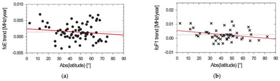
Figure 1. foE (dots) (a) and foF1 (x) (b) trends in terms of absolute value of the latitude of the individual stations. The dashed lines characterize the mean global foE and foF1 trends, the full lines are the curves of the best linear fit through the individual trend values. (Reproduced from Bremer [41]: Figures 6 and 10, modified).

Jarvis [42], in his study of foE trend variation across stations in Europe, is the only paper analyzing in depth the possible ways in which Earth’s magnetic field’s secular variation could affect E-region electron density. Even though the results are for mid-latitude stations and the final conclusions are that it seems very unlikely that the geomagnetic secular variation is the root cause of the differential trends, we consider it is worthwhile mentioning them since they may also apply to lower latitudes. These conclusions are the following:

• Changes in the auroral ovals, which may result in an increase or decrease of a station’s position relative to the auroral oval. This is linked to an increase or decrease, respectively, of energetic charged particles’ precipitation from the magnetosphere which in turn generate nitric oxide (NO) that at E-region altitudes can produce an increase in ionization loss rate and hence a decrease in the E-region electron concentration.
• The ratio of the geomagnetic field strength at 110 km to that at equatorial minimum on the same field line determines the particle loss cone, which could affect foE also through changes in charged particle precipitation.
• The dip angle and declination could have a more direct effect on foE because they have some controlling influence over plasma motion, even though they really become effective at the F2 layer, where transport processes gain importance in the continuity equation.
• Geomagnetically, conjugate points to a given station may be changing their latitude in the opposite hemisphere and hence altering the secondary ionization being transported along the field line between hemispheres.

It is also worth mentioning the work by Venkat Ratnam et al. [43] for their analysis of temperature and wind trends in the low-latitude middle atmosphere with observations from several instruments and satellite data over the Indian region, combined with Whole Atmosphere Community Climate Model eXtension (WACCM-X) simulations. They conclude that “it is clear that the effects of the anthropogenic changes in the lower atmosphere are clearly reflected in the complete middle atmosphere over the low latitudes.” The weak or maybe null role of the Earth’s magnetic field variation may contribute to the clearer picture here than in upper regions.

3.3. Ionospheric F2-Layer Peak Electron Density and Height

At the F2-layer the situation completely changes since transport becomes a key factor in the continuity equation. Equation (1) is clearly reflecting that something must happen in response to magnetic field variations that result, at least, in D and I change. However, there are not many works based on stations’ experimental data dealing in particular with equatorial and low latitudes. This may be due to their relatively very low amount in comparison to mid- and high-latitude ionospheric stations.

An interesting study is that by Scott and Stamper [44] which analyzes long-term changes in the relative magnitude of the annual and semi-annual variations in foF2 through the power ratio of each component using 77 ionospheric stations around the world (from which 7 to 10 are located at equatorial and low latitudes). Their hypothesis is that the relative contribution of annual and semi-annual components at a given station has varied since ionospheric records began in the 1930s in the same way as the whole upper atmosphere has along these decades in response to increasing greenhouse gases concentration and other long-term trend forcings.

The F2-layer seasonal variation presents temporal and spatial variations, changing from annual to semiannual patterns depending on altitude, latitude, longitude, local time, and the phase of solar cycle; and although it has been studied for decades, it is still a question not fully solved. Historically, when the F2 layer behavior significantly deviated from the solar zenith angle dependence, they were called ‘anomalies’. Typical anomalies are the seasonal or winter anomaly (NmF2 greater values in winter than in summer) and the semiannual anomaly (greater NmF2 at equinox than at solstice).

Scott and Stamper [44] observe that the global variation in foF2 long-term annual variability shares regional similarities with global trends seen in hmF2 long-term changes. Since both parameters are influenced by thermospheric composition and circulation, they argue that both mechanisms may be responsible for the observed variability and suggest that the full understanding of their role in trend analysis could be done through a precise modeling for each location using a global coupled thermosphere-ionosphere model similar to the one used by Millward et al. [45]. This model demonstrates that the variability of foF2 along the year can be explained by changes in thermospheric composition, which in turn is influenced by the proximity to the geomagnetic pole, and also on ion production rate that depends on solar zenith angle.

Even though Scott and Stamper [44] consider the secular geomagnetic field variations as a feasible trend forcing mentioning in some detail its role producing trends, they do not delve into this argument. Regarding this, they just conclude that: “This work once again highlights the potential for long-term change in a global parameter to generate a range of localized responses in the ionosphere.”

Danilov [46,47] and Danilov and Vanina-Dart [48,49] analyze the foF2 noon–night correlation and ratio as proxies for thermospheric dynamics considering low-latitude stations. Their main idea is that daytime foF2 values are mostly not sensitive to dynamical processes and are governed mainly by the photochemical processes balance, whereas at night, when ionization by direct solar radiation is absent, the impact of dynamical processes due to the horizontal wind leading to a vertical shift of the F2 layer, may become quite substantial. A result we would like to highlight is that the difference in the sign of trend values is argued to be related to trends in the vertical drift which depends directly on the zonal and meridional winds together with D and I. Even if the trend sign is pointed out to depend on D and I value, and not on their secular variation, an implicit role of the Earth’s magnetic field changes can be hinted at.

Gnabahou et al. [50] analyzed foF2 long-term variability at Ouagadougou (12.4° N, 358.5° E), which is a West African equatorial station. Considering annual mean data series at 12 LT for the period 1966–1998, a downward trend of −0.015 MHz/year is obtained, qualitatively consistent with a decreasing trend expected from increasing greenhouse gas concentration but much greater. In trying to elucidate this lack of quantitative agreement, they find that it cannot be explained either by the secular variation of I at Ouagadougou location, but with an additional mechanism instead: the secular movement of the dip equator toward Ouagadougou, which can be appreciated from Figure 2, and which implies an approach of the EIA trough. This last mechanism yields an foF2 decrease which should be added to the greenhouse gases effect with a final better agreement with the experimental decreasing trend obtained. Of course, the competing two roles of the geomagnetic field secular variation in this case, one through D and I variation and the other through the EIA displacement effect, should be considered together.

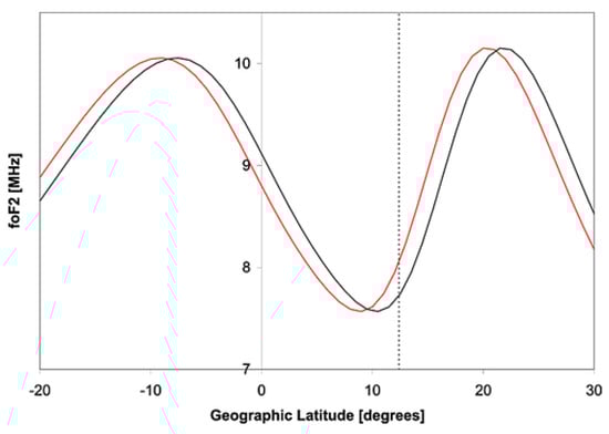
Figure 2. Latitudinal profile of foF2 at the geographic longitude of Ouagadougou (358.5° E) obtained with the International Reference Ionosphere model, IRI2007, as an example for January, at 12 LT, and solar activity level corresponding to F10.7 = 150 (red line). foF2 profile displaced according to the displacement of the magnetic dip equator at the Ouagadougou longitude (black line). The dotted vertical line indicates the latitude of Ouagadougou. (Reproduced from Gnabahou et al. [50]: Figure 5).

This work expands its analysis of the secular variation geomagnetic field effects over low latitudes also analyzing the results by Ouattara [51] for additional local times in terms of EIA latitudinal profile, which accompanies the dip equator movement at Ouagadougou longitudinal position.

In a similar work, Pham Thi Thu et al. [52] analyzed foF2 long-term trend measured at Phu Thuy (21.03° N, 105.96° E), Vietnam, located under the northern crest of EIA considering annual mean data at 04 LT and 12 LT for the period 1962–2002. In both cases a positive trend was obtained, not consistent with the greenhouse gases effect. The increasing trend observed at 12 LT is qualitatively in agreement with the expected effect of the secular displacement of the dip equator over the EIA latitudinal profile, while, at 04 LT, when the EIA is absent, the positive trend is in qualitative agreement with the secular variation of I, and the consequent increase of the sin(I)cos(I) factor at the corresponding location, as deduced from Equation (1).

In both works, [50,52], results for Huancayo (12.0° S, 284.7° E) and Phu Thuy (21.03° N, 105.96° E) obtained by Upadhyay and Mahajan [53] and Pham Thi Thu et al. [54], respectively, are also explained in terms of the EIA latitudinal profile displacement. Huancayo is, like Ouagadougou, an equatorial ionospheric station north of the dip equator, but in the southern hemisphere. The dip equator is moving away from the station, so an increase in foF2 should be expected as the trend obtained by Upadhyay and Mahajan [53]. In this case the positive trend is also in agreement with the decrease of the sin(I)cos(I) factor at the corresponding location.

3.4. Topside Ionosphere

As Cai et al. [55] mention in their work, little attention has been paid to the topside ionosphere trend. Their study is the first to analyze in situ data measured by the Defense Meteorological Satellite Program (DMSP) satellites in order to derive the long-term trend of the topside ionosphere using techniques of artificial neuron network and multiple linear regression methods for the period 1995–2017. They obtain in this case positive and negative electron density trends at middle and low latitudes, at ~860 km, ranging from ~−2 to ~+2% per decade, with clear seasonal, latitude, and longitude variations. In order to detect their origin, a series of control simulations based on the Thermosphere-Ionosphere Electrodynamic General Circulation Model (TIE-GCM) driven by the realistic long-term changes in CO₂ and the geomagnetic field, was implemented to compare with the observational results.

Their final conclusion is that the long-term geomagnetic field variation is most likely the dominant factor controlling the long-term trend they obtained, without discarding, however, the CO₂ long-term enhancement role.

3.5. Ionosphere Total Electron Content (TEC)

Lean et al. [56] were the first to analyze TEC trends using data obtained from multiple GPS observations between 1995 and 2010. They conclude their results with a global positive trend of +0.6 TECU (TEC Units = 10¹⁶ electrons/m²) per decade, in disagreement with the negative mean value expected from a purely greenhouse effect. However, a regional dependence of TEC trends magnitude is also shown with a strong association with Earth’s magnetic field, as can be noticed from Figure 3. This trend is estimated from a multiple regression model adjusted to TEC data series which explicitly includes time as a variable.

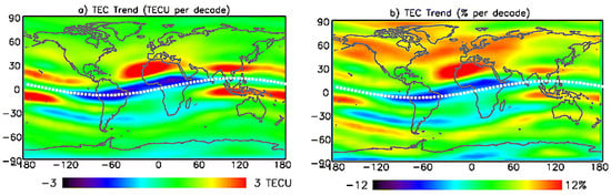
Figure 3. (a) The geographical distribution of 1998–2010 TEC trends obtained using the 3C model of EUV irradiance variability as absolute values in TEC units. The trend values have been normalized so that the global mean trend is +0.6 TECU per decade (the average of the 1995–2010 global trends using the 2C and 3C models). (b) Percentage changes relative to the average ionosphere. (Reproduced from Lean et al. [56]: Figure 7, modified. See [56] for details on EUV (extreme ultraviolet) modeling).

Zonal bands of alternating stronger and weaker TEC trends are shown approximately parallel to the magnetic dipole equator. Regionally, TEC trends are largest where the dipole and dip equators diverge. Positive TEC trends in excess of +3 TECU per decade are located over the eastern Atlantic Ocean and western Africa in the mid-latitude Northern Hemisphere; negative trends in excess of −3 TECU per decade occur over South America and equatorial Atlantic and Africa, between the magnetic and dip equators.

In a later work, Lean et al. [57] analyzing a longer TEC database covering the period 1998 to 2015, with a different approach obtained a similar regional pattern for trend values, but a statistically non-significant global trend, with a slightly negative value (−0.15 TECU per decade). In this case, instead of including the trend in the model, they estimate it from the residuals of TEC observations and model. Again, the spatial pattern of the linear trend has alternating bands of positive and negative values, very similar to that shown in Figure 3, and aligned with the equatorial ionization anomaly that are as much as an order of magnitude larger than the globally averaged rate of change. The difference with Lean et al. [56] is that in this previous case there were more regions having positive than negative trends.

Lastovicka [58] analyzed the contradictory result with the greenhouse hypothesis for the global average TEC trend, and more recently Lastovicka et al. [59] extended this analysis to longer TEC records but considering global average values with which the positive and negative trends alternation at equatorial and low latitudes is blurred out.

Andima et al. [60] analyzed TEC trends for Malindi, Kenya (3.0° S, 40.2° E) for the period 1999–2017, and also for the African low latitude region, using GPS-derived TEC. They obtain a latitudinal pattern similar to that shown in Lean et al. [56,57], with positive as well as negative trends, and they mention the possibility of the secular Earth’s magnetic field changes as a source. However, they do not explore this possibility and propose it for future studies.

3.6. Ionospheric Currents: Sq and EEJ

The first results on trends in ionospheric currents linked to the Earth’s magnetic field secular variation, where data measured at low latitudes are used, are those by Sellek [61] and Schlapp et al. [62]. In particular, Sellek [61] analyzed Sq currents trend and finds significant secular changes for Huancayo (12.0° S, 284.7° E), Hermanus (34.4° S, 19.2° E), and San Juan (18.1° N, 293.8° E) that appear to result from changes in the Earth’s main magnetic field. In the case of Huancayo, the trend is also related to the equatorial electrojet secular displacement.

In a much later work, Elias et al. [63] obtained significant increasing trends in the daily range of the Sq variation of H measured at Apia (13.8° S, 188.2° E), Fredericksburg (38.2° N, 282.6° E), and Hermanus (34.4° S, 19.2° E). In the cases of Fredericksburg and Hermanus, more than half of the observed trends may be accounted for by B secular variations in the respective sites through the direct effect over the ionosphere conductivity above each location. The expected effect of greenhouse gases increase would be an increase on electron density which implies an increase also in Sq through its effect over current density. In the case of Apia, its closeness to the equatorial electrojet may add an additional influence on H behavior. However, Elias et al. [63], in a preliminary test for this possibility, find that there should not be any noticeable effect.

de Haro Barbas et al. [64] added two additional equatorial station: Bangui (4.4° N, 18.6° E) and Trivandrum (8.5° N, 77.0° E), with a similar analysis to that of Elias et al. [63] but adding a comparison with simulations using the Coupled Magnetosphere-Ionosphere-Thermosphere (CMIT) model. A general qualitative agreement between experimental trends in Sq amplitude and the trends in B was observed, which suggests that the change in B, through its influence on the ionospheric conductivity, is again the main cause of Sq amplitude trends, and not the equator displacement.

Shinbori et al. [65] analyzed the characteristics of long-term variation in Sq amplitude geomagnetic field data obtained from 69 worldwide geomagnetic observation stations within the period 1947–2013. In addition to the dependence on the 10- to 12-year solar activity cycle, they obtained long-term trends after filtering the solar activity effect which were mostly negative over a wide region, as can be noticed from Figure 4. They observe that this tendency was relatively strong in Europe, India, the eastern part of Canada, and New Zealand. The relationship between the magnetic field intensity at 100 km altitude and residual Sq amplitude showed an anti-correlation for about 71% of the geomagnetic stations. Furthermore, the residual Sq amplitude at the equatorial station of Addis Ababa was anti-correlated with the absolute value of the magnetic field inclination. This implies movement of the equatorial electrojet due to the secular variation of the ambient magnetic field.

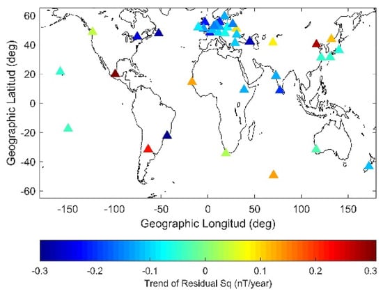
Figure 4. Global distribution of 40 residual Sq trends that passed through a trend test as a function of geographical latitude and longitude. (Adapted from Shinbori et al. [65]: Figure 8).

Moving now to a station located at the magnetic equator, Matzka et al. [11] analyzed the sensitivity of the equatorial ionospheric current system (the Sq and EEJ systems) to solar cycle variations and to the secular variation of the geomagnetic main field, considering 51 years (1935–1985) of data from Huancayo (12.0° S, 284.7° E). They observe that this period is ideal to analyze the influence of the main field strength on the amplitude of the quiet daily variation, since the main field decreases significantly from 1935 to 1985, while the distance of the magnetic equator to the observatory remains stable. In fact, we consider that it is this last mechanism which induces the stronger trends. They confirm an increase of ΔH for the decreasing main field in this period, as expected from physics-based models, but with a somewhat smaller rate than predicted.

Soares et al. [66], noting that the magnetic equator in the Brazilian region has moved over 1100 km northward since 1957, passing the geomagnetic observatory Tatuoca (1.2° S, 311.5° E) in northern Brazil, analyzed ΔH from 1957 until 2019, detecting the trend expected from the main field secular variation and corroborated by TIE-GCM simulations. In addition, the effect of the magnetic equator displacement along the Tatuoca meridian is perfectly noted since until the 1990s, ionospheric solar quiet currents dominated the quiet-time daily variation at this geomagnetic observatory and after 2000, the magnitude of the daily variation became appreciably greater due to the EEJ contribution.

In a different kind of analysis, but considering also that above certain regions in Brazil, the magnetic dip equator movement is the fastest over the low latitude region of the globe, Moro et al. [67] analyze its impact on the EEJ through the effects over electric fields inferred from coherent radar data in the E region (which they call “E-region electric fields—EEF”). They point out that the magnetic equator secular displacement in the Brazilian longitude sector is fast enough to cause changes in this electric field that can be observed in the time scale of a solar cycle or less. For this purpose, the authors analyze the seasonal variability of EEF in a station in Brazil (Sao Luis Space Observatory (SLZ), 2.3° S, 315.8° E) and a station in Peru (Jicamarca Radio Observatory (JRO), 11.9° S, 283.1° E) obtained from radar soundings collected from 2001 to 2010. Among other results, they observed an EEF seasonal difference between these two sectors in South America: EEF is more intense in summer at SLZ and in equinox at JRO due to the different declinations in each observatory. The slow westward movement of the declination pattern is mentioned, which is mainly apparent in the east coast of Brazil at middle and equatorial latitudes, but not further analyzed. In addition, EEF has been highly variable with season in the Brazilian sector compared to the Peruvian sector due to the magnetic equator displacement, which is almost static above Peru, but is displacing relatively fast above Brazil. In addition, this displacement would be affecting the time span along which the EEJ is observed. In the case of SLZ in Brazil, above which the magnetic equator is moving farther away, the EEJ is being observed later and ends sooner, that is reducing its time duration.

3.7. F3 and Sporadic E Layers

Batista et al. [68] analyzed 25 years of data recorded over Fortaleza (3.8° S, 321.6° E) since 1975 until 2000, to investigate how the F3-layer occurrence varied with changes in I and in solar activity. Accompanying the magnetic equator secular displacement, I angle over Fortaleza varied from 1.7° S in 1975 to 11° S in 2000 (a rate of approximately ~22’/year). F3 layer frequency occurrence data indicate that it increased with increasing I (that is the station is “moving” away from magnetic equator) during the periods of low and high solar activity, in agreement with theoretical studies.

To this result, we add that obtained by Abdu et al. [69], where long term trends in the sporadic E (Es) layers occurrences measured at Fortaleza were analyzed using 16 years of data (from 1975 to 1990). The secular drift of the magnetic equator and hence that of the EEJ along Fortaleza’s meridian was detected as the main source of the long term changes observed in Es-layers occurrence.

With these results, we want to highlight again the effect of the magnetic equator over the ionosphere. In this case, it is important to note that this equator, in its slow movement due to the secular variation of the geomagnetic field, induces phenomena that are not usually observed unless we are located at or very close to the magnetic equator. Their importance resides in that they are very likely to affect telecommunications and GPS signals, and are therefore important for space weather considerations.

3.8. Warnings for Experimental Trends’ Assessment

Given the importance of the estimated trends’ values, we consider it important to mention in this review the warnings about estimation methods.

Trend estimation from experimental data is subject to major problems due to the methodology used to extract trend values and/or the data characteristics. The first is due mainly to the need of filtering effects of forcings which are much stronger than the expected trends and the latter is due to the needed time length of data (exceeding ~20 years) which entails, in addition to the usual data requirements, the need to check data homogeneity and also the higher chances for data gaps. A fairly complete analysis of these issues, which apply to the whole ionosphere, was done by Lastovicka [7], in his Section 17.2 (entitled precisely “Various problems of trend investigations”) with many references to each aspect regarding methodological and data warnings.

In addition to the more specific works cited by Lastovicka [7] on each of the numerous aspects that he considers about long-term trend assessment from upper atmosphere experimental data, we add the followings: Elias [70] with a fair complete analysis of some risks in trend estimations when filtering solar activity effect from F2 region data, and a set of three papers by Lastovicka [71,72,73] dealing with the solar proxy selection to effectively and efficiently filter solar activity effect from E- and F-layer parameters.

The works by Danilov and Mikhailov in collaboration and with other authors [74,75,76,77,78] dealing with the geomagnetic activity control of ionospheric trends are also worth mentioning. Even if equatorial and low latitudes may not significantly suffer these consequences, the geomagnetic activity control indirectly points at a geomagnetic field effect through the dependence of geomagnetic storms geo-efficiency according to relative location with respect to regions highly affected by energetic particle injection. In fact, these works highlight an inherent geomagnetic control which cannot be easily filtered in order to detect trends due to other sources.

4. Long-Term Trends Based on Theoretical Analysis and Modeling

The results obtained from physical considerations and modeling were also a starting point for the analysis of trends connected to the geomagnetic field secular variations, whose initial “kick”, according to us, was that by Foppiano et al. [79].

Due to the ionospheric system complexity when its dynamics is fully included, as should be done if the geomagnetic field effects are trying to be detected, a usual way to do it is to simplify the magnetic field configuration. The natural choice for this is to consider a pure dipolar field, taking into account that it can explain ~80% of the present field, in addition to the very weak and slow variation of the multipolar components. However, there are models which consider the “true” Earth’s magnetic field with all its complexity.

We describe in this section the modeling results which include equatorial to low-latitude ionospheric regions, separated according to the Earth’s magnetic field model they include in the simulations, which are: the “real” field obtained from the International Geomagnetic Reference Field model (IGRF) [80] and a pure dipolar field.

4.1. Modeling Using IGRF

Cnossen and Richmond [38] were the first to quantify the global effects of magnetic field changes on the ionospheric F2 layer using simulations from TIE-GCM, which uses the IGRF to define the magnetic field in the model. They observed that changes are very small in most regions as can be noticed from Figure 5 and Figure 6. However, a strong spatial dependence is seen, accompanied by variations also (even in sign) with the season and time of day. In fact, they become much larger over the Atlantic Ocean and South America, roughly from 50° S to 50° N and 90° W to 10° E. This region is the same where the change in the sin(I)cos(I) factor has its largest magnitudes. Near the equator changes in hmF2 reach up to ±20 km (~5%) and changes in foF2 up to ±0.5 MHz (~10%) for most seasons and times of day, and in some cases even larger changes can be found.

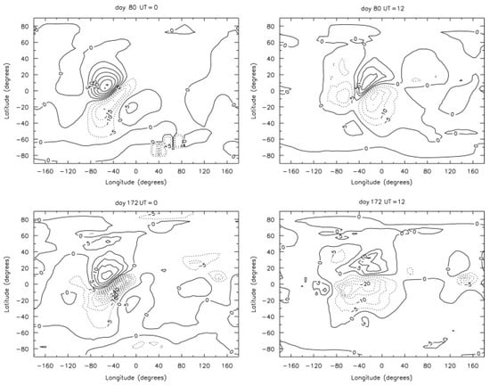
Figure 5. Global change in hmF2 (km) at day 80 (top) and day 172 (bottom) at 0 UT (left) and 12 UT (right) between 1997 and 1957 (1997–1957). (Reproduced from Cnossen and Richmond [38]: Figure 5).

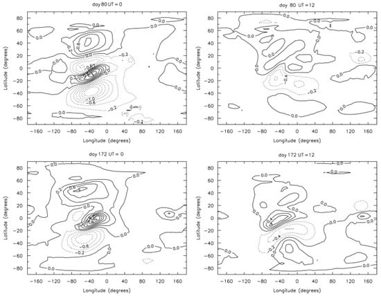
Figure 6. Global change in foF2 (MHz) at day 80 (top) and day 172 (bottom) at 0 UT (left) and 12 UT (right) between 1997 and 1957 (1997–1957). (Repdroduced from Cnossen and Richmond [38]: Figure 6).

With a much simpler approach, Elias [8], considering just first approximations already used in Elias and Adler [37], and using IGRF to model the Earth’s magnetic field variation over hmF2 and foF2 through its effects on ionization transport, obtained similar trend spatial patterns to Cnossen and Richmond [38]. These are in agreement also with some values obtained with experimental data. This simple approach can give a first picture comparable to that obtained using much more complex models; however, it should be taken into account that several factors are not considered, such as coupling mechanisms and long-term variations in the wind strength, neutral composition, and temperature. Despite the disadvantages, this simple approach allows to visualize, in a first approximation, the role of the variables considered. Again, the stronger trends are obtained for equatorial to low latitudes, in the longitudinal region coincident with Cnossen and Richmond [38].

Cnossen and Richmond [81] added to the previous study the analysis of Sq using the CMIT model, where the magnetosphere role is included now. Their simulations were done considering the magnetic fields of 1908, 1958, and 2008 from IGRF. The strongest differences occurred between ~40°S–40° N and ~100°W–50° E, which they refer to as the “Atlantic region”, as can be noticed in Figure 7. The changes in hmF2 and foF2 are produced by a combination of changes in the vertical E × B drift and the vertical components of plasma diffusion and transport by neutral winds along the magnetic field. Changes in hmF2 are considerably stronger during the day than at night, while changes in foF2 are only somewhat smaller at night.

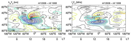
Figure 7. Maps showing the difference of the 15-day mean hmF2 (left) and foF2 (right) in 2008 with 1908 at 14:00 UT. Light (dark) shading indicates 95% (99%) statistical significance. (Reproduced from Cnossen and Richmond [81]: Figure 3, modified).

Regarding the amplitude of the Sq magnetic variation, the strongest changes occur near the magnetic equator, as noticed from Figure 8, and are mainly associated with the northward movement of the magnetic equator in the Atlantic region and the westward drift of the magnetic field. Changes in magnetic field strength seem to be relatively less important at low magnetic latitudes. In the Atlantic region, simulated trends in hmF2 and foF2 are comparable in magnitude to observed trends and are ~2.5 times larger than trends predicted from the increase in greenhouse gas concentrations. Moreover, simulated trends in Sq amplitude are comparable to, or even somewhat larger than, typical observed trends in the Atlantic region. Earth’s magnetic field secular variation may therefore be the dominant trend source in the Atlantic region ionosphere, while being less important in other world regions.

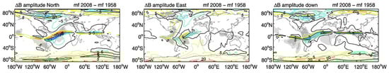
Figure 8. Map showing the difference of the 15-day mean northward (left), eastward (middle), and downward (right) component of the daily Sq amplitude in 2008 and 1908. Light (dark) shading indicates 95% (99%) statistical significance. (Reproduced from Cnossen and Richmond [82]: Figure 9, modified).

Changes in hmF2 and foF2 are similar to those obtained in their previous work [38] with TIE-GCM, but there are some differences in the day and night responses variations, and the longitude range of the strongest trends, which is wider in the CMIT case. They argue that a possible cause for this may be the different solar activity levels of the simulations, being greater in Cnossen and Richmond [38] (F10.7 = 150) than in Cnossen and Richmond [81] (F10.7 = 70).

Cnossen [10] used the WACCM-X to consider realistic variations in solar and geomagnetic activity, the Earth’s magnetic field, and trace gas emissions, including CO₂, for the period 1950–2015. Trends due to Earth’s magnetic field secular variation were obtained through a multiple linear regression fitting to the modeled output values where solar activity and geomagnetic activity were considered through F10.7 and Kp indices. Focusing on the trend spatial variation, they observed some relatively large low-latitude changes in Joule heating power at ~60–0° W, as can be seen in Figure 9 clearly associated with the relatively large movement of the magnetic equator in this longitude sector. However, they note that they are unlikely to have a significant effect on the thermosphere temperature, as the absolute magnitude of the Joule heating power at low latitudes is much smaller than at high latitudes.

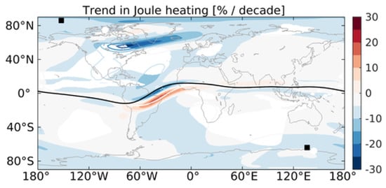
Figure 9. Trend in vertically integrated Joule heating power (%/decade) calculated with linear regression Model 3. Filled contours indicate that trends are statistically significant at the 95% confidence level, while line contours are used for non-significant trends. The location of the magnetic equator and magnetic poles in 1950 (2015) are marked with a white (black) line and white circles (black squares), respectively. (Reproduced from Cnossen [10]: Figure 4).

Figure 10 shows maps of the long-term trends in hmF2 and NmF2. They mention that the spatial pattern of trends in TEC looks very similar in structure to that of the trends in NmF2. The spatial structure of trends indicates a superposition of CO₂ and magnetic field effects. The low-to mid-latitude trends around ~60° W to 20° E are clearly associated with main magnetic field changes (especially the movement of the magnetic equator), matching quite well with expectations from previous modeling studies [38,81].

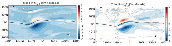
Figure 10. Trends in hmF2 (km/decade, left) and NmF2 (%/decade, right). Filled contours indicate that trends are statistically significant at the 95% confidence level, while line contours are used for non-significant trends. The location of the magnetic equator and magnetic poles in 1950 (2015) are marked with a white (black) line and white circles (black squares), respectively. (Reproduction from Cnossen [10]: Figure 5).

4.2. Modeling Using a Pure Dipolar field

Yue et al. [82] claim to be the first in using a middle- and low-latitude ionospheric theoretical model to assess the effects of the secular variations of geomagnetic field orientation on ionospheric long-term trends. They consider a theoretical model that solves plasma continuity, motion, and energy equations simultaneously and uses an eccentric dipole approximation for the Earth’s magnetic field. Solar and geomagnetic activities are kept constant at middle and quiet levels, respectively, while changes of geomagnetic field elements, including the center location of the dipole field, I and D, and geomagnetic latitude and longitude, are calculated by the IGRF spherical harmonic coefficients during the years 1900–2005 with a 5-year interval. Twelve artificial stations, which are distributed over four typical longitudinal sectors are selected in this modeling, with three stations in each longitudinal sector which represent the northern low latitude (~geomagnetic 20°), equatorial area (~geomagnetic 0°), and southern low latitude (~geomagnetic −20°), respectively. The long-term variations of modeled foF2 and hmF2 over the 12 selected locations from 1900 to 2005 present notable regional characteristics because of the differences of geomagnetic field trends among different stations. They have bigger amplitudes in the 320° longitude sector than in the other three longitude sectors, the same as that of I and D, with seasonal and daily typical regional characteristics. They notice a difference between equatorial and low latitudes: because of the configuration of the geomagnetic field, the diffusion of the plasma is mainly horizontal at the equatorial station, but with the increase on latitude, the vertical component of diffusion becomes important. Therefore, the trends of foF2 and hmF2 should present a behavior like that of cos(D)cos(I) in the equatorial stations and like that of the amplitude of cos(D)cos(I)sin(I) in the higher latitude stations. In fact, it is observed that the sign of foF2 trends for low-latitude stations agrees well with that of |cos(D)cos(I)sin(I)|, while the sign of foF2 trends in the case of equatorial stations is in agreement with that of |cos(D)cos(I)|. In the situation of hmF2, there is also a general agreement with the above theoretical interpretation.

Batista et al. [83] analyze the effect of the vertical plasma drift and thermospheric wind over the equatorial ionization anomaly using the Sheffield University Plasmasphere-Ionosphere Model (SUPIM) together with the effect of the magnetic field secular variations on the EIA location over the Brazilian region. The geomagnetic field is represented by a tilted centered dipole with the angle of tilt and D given by IGRF. In order to ensure that the changes observed were due to the secular variation in the geomagnetic field alone, all other input parameters (such as vertical drift, solar flux, neutral wind, and geomagnetic activity) were kept unchanged from one run to the other. They observed that I over northeast Brazil varies at a rate of 20′/year, corresponding to an apparent northwestward movement of the magnetic equator, which should affect EIA position. From the simulation results of the F region plasma frequency in terms of latitude at 45° W position, they determined the EIA crests and troughs for high and low solar activity years (1978, 1989, and 2002, and 1986, 1996, and 2006, respectively), finding that they are all moving northward: from ~25° S to ~21° S between 1978 and 2002 in the case of the southern crest, and from ~5.5° N to ~10° N in the northern case. The same rate of change, but slightly different results were obtained in the case of years of minimum solar activity levels. This can be clearly seen in Figure 11, which shows the crest position at the southern hemisphere for high and low solar activity together with the magnetic equator position. The geographic latitude of the EIA crest varies at a rate of 10’/year and 9.5’/year for the high and low solar activity periods, respectively, which are very close to the rate of change of the dip equator at the same meridian that is equal to 11.6’/year, according to IGRF results. This means that the EIA practically follows the magnetic equator in its secular movement.

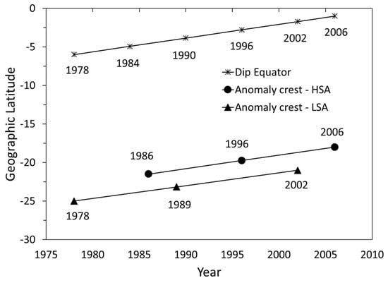
Figure 11. Time variation of the geographic latitude of the EIA crest at the southern hemisphere, over the 45° W meridian high solar activity (HSA) (triangles) and low solar activity (LSA)(circles). The time variation of the geomagnetic equator position at the same longitude is also shown (stars). (Adapted from Batista et al. [83]: Figure 8).

Cnossen and Richmond [18] investigated, in particular, the effects of changes in dipole tilt angle using the CMIT model. This angle was varied from 0° to 60° to study its role in the mesosphere-ionosphere-thermosphere (MIT) system, keeping the longitude of the geomagnetic pole in the northern hemisphere fixed at 70° W, and the dipole moment set to 8.0 × 10²² Am². The F10.7 value was set at 150, which corresponds to medium solar activity levels. Even though the simulated changes are much stronger than the true secular change, they may be indicative of the results expected for smaller variations.

This work introduces the effect of interplanetary magnetic field (IMF) considering scenarios for northward and southward IMF, that is minimum and maximum solar wind-magnetosphere coupling, showing three mechanisms through which a change in dipole tilt angle can affect the MIT system: changes in the amount of Joule heating through variations in solar wind-magnetosphere coupling efficiency, changes in the geographic distribution of Joule heating and magnetospherically driven ion convection patterns through changes in magnetic pole positions, and changes in vertical plasma transport through changes in the inclination of the magnetic field at a given geographic location. They show that each of these mechanisms contributes to the response of the MIT system to a change in tilt angle.

From Figure 12, showing the different scenarios considered, apart from the strong change in the polar regions, it is evident that stronger changes should be expected at the magnetic equatorial region considering its strong displacement. In our case, the most important consequence is linked to changes in the filed lines’ tilt angle, that is the change in the orientation of magnetic field lines at a given geographic location.

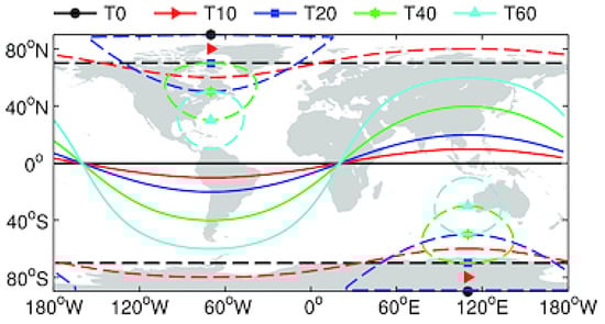
Figure 12. The locations of the magnetic poles (markers), the approximate locations of the polar caps (dashed lines), and the location of the magnetic equator (solid lines) for tilt angles of 0, 10, 20, 40, and 60° (labeled as T0, T10, etc.). The longitude of the Northern Hemisphere (NH) magnetic pole was set to 70° W in all cases, and correspondingly, the longitude of the Southern Hemisphere (SH) magnetic pole was set to 110° E. The polar caps were approximated as circles with a 20° radius around the magnetic poles (distortion of the circular shape is due to the projection). (Reproduced from Cnossen and Richmond [18]: Figure 1).

The magnetic field orientation is important for the ionosphere because its charged particles moves much more easily along field lines. In this case, there are in addition changes in D which will also contribute to transport variations as can be deduced from Equation (1).

Going to Cnossen and Richmond [18] results for low and equatorial latitudes, they observe first that for all scenarios hmF2 and NmF2 are organized by magnetic latitude, and that hmF2 presents the largest values at the magnetic equator, while a double-peak structure can be seen in NmF2, with maxima on either side of the magnetic equator. The longitudinal variation in hmF2 and NmF2 increases as the dipole tilt increases. In fact, the original pattern becomes gradually more distorted since it follows magnetic latitudes which become more undulating. This produces an alternating pattern of increases and decreases on either side of the geographic equator as can be noticed in Figure 13.

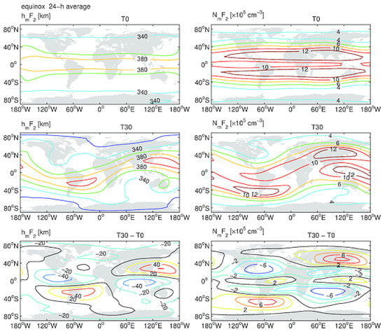
Figure 13. Maps of the 24-h mean height of the F2 peak, hmF2 (km), and the peak electron density of the F2 layer, NmF2 (×10⁵ cm⁻³) for T0, T30, and the difference (T30–T0) for March equinox and southward IMF. (Reproduced from Cnossen and Richmond [18]: Figure 7).

They analyze three possible sources for this: (1) the difference in the O/N₂ ratio, related to the neutral wind circulation, which is a measure of ion production versus ion loss processes, and which may explain some of the changes in NmF2, (2) neutral winds that can also directly affect the vertical distribution of ionospheric plasma through the mechanism explained in Section 2.3.1; and (3) diffusion along magnetic field lines, where gravity is the main driving force, so that the plasma generally diffuses downward along the inclined magnetic field lines. The last mechanism acts to decrease hmF2 directly and also reduces NmF2 by bringing down the plasma into regions where more recombination takes place. Only at very low magnetic latitudes, where the magnetic field is essentially horizontal, plasma diffuses mainly horizontally, away from the magnetic equator. The lack of downward diffusion at low magnetic latitudes is the main reason that hmF2 and NmF2 are highest near the magnetic equator, as already mentioned in the EIA explanation of Section 2.1.

Because the magnitude of the vertical diffusion velocity depends directly on I, the diffusion patterns follow magnetic latitudes, with the weakest diffusion occurring at the magnetic equator. The difference in vertical diffusion velocity spatial pattern is seen in Figure 14 which, at mid to low latitudes is very similar to the difference pattern in hmF2, and somewhat similar to the difference pattern in NmF2. Cnossen and Richmond [18] conclude: “It is therefore likely that changes in vertical diffusion play a significant role in hmF2 variation, and to a lesser extent in the NmF2 case.”

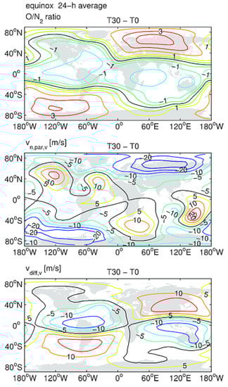
Figure 14. Maps of the difference (T30–T0) of the 24-h mean O/N₂ ratio, the vertical component of the plasma transport by neutral winds along magnetic field lines, v_n,par,v (m/s), and the vertical component of the plasma diffusion along magnetic field lines, v_diff (m/s) for March equinox and southward IMF. Both velocities are positive upwards. All maps are at a constant pressure level of 3.2 × 10⁻⁸ hPa, corresponding roughly to the level of the F2 peak height. (Reproduced from Cnossen and Richmond [18]: Figure 8).

More concentrated on conductivity and currents, Tao et al. [84] investigate the effect of the intrinsic magnetic field on a coupled system, especially focusing on the low- to mid-latitude thermosphere dynamics, using the numerical model GAIA (Ground-to-Topside Model of Atmosphere and Ionosphere for Aeronomy). This model solves the physical and chemical processes of the whole atmosphere from the troposphere to the exosphere including the interaction with the ionosphere. GAIA incorporates meteorological reanalysis data at low altitudes (<30 km), which enables to investigate the atmospheric response under the existence of various realistic waves. They used a tilted dipole magnetic field in the model, with an initial dipole moment of 7.8 × 10²² Am² which is reduced to 75, 50, and 10% of this value. Solar low and quiet activity was considered (F10.7~70 and Kp < 3).

Key observations are the increase in the height of the conductivity peak with B decrease, due to the mechanism explained in Section 2.3.2 (that is, the induced cyclotron frequency decrease which implies an upward shift of the peak conductivity layer to heights where the cyclotron frequency and the collision frequency become comparable again). Since the ion density increases with altitude up to the F2 peak at ~400 km, the conductance increases considerably with decreasing magnetic field. They show global values variations, which blurs the equatorial and low-latitude changes, but also zonal mean values which emphasize them.

A new result, which deserves to be highlighted in this work, is the effect on superrotation. When the magnetic field decreases, several waves are amplified at high altitudes. The reduced constraint on the plasma motion by a small magnetic field causes a small drag effect, resulting in a large neutral velocity and a large wave amplitude. The resulting westward acceleration of the equatorial neutral wind jet decreases the superrotation velocity by ~20% when the intrinsic magnetic field is reduced to 10%. The reduced constraint on the ion motion by a small magnetic field causes a large ion drag effect, resulting in the westward acceleration of the neutral wind. Again, even though these variations are enormously exaggerated compared to the true secular variation along the last 120 years, they are indicative of what is going on, even though very weakly, and what to expect in a transitional scenario.

4.3. Warnings for Theoretical and Model Trends Assessment and Simulations

Models in general are based on simplifications of the system we want to study. In our case, one of main simplifications is the Earth’s magnetic field model used, which in general is the pure dipole approximation. During the last decades, and surely for many decades more in the future, it will still be a good approximation as long as we consider the secular variation in its tilt angle with respect to the Earth’s rotation axis and its center displacement. These two effects seem to induce stronger effects at the equatorial and low-latitude regions than changes in the field intensity.

Another aspect to be warned of is the models’ complexity degree and the inclusion or not of the magnetosphere coupling. We consider that for the study of regions far from high geomagnetic latitudes, this additional complexity could be simplified or even neglected. This will not be possible of course during transitional field scenarios where a multipolar field could prevail with plausible auroral zones in geographic low-latitude regions [85].

5. Conclusions

Long-term trend studies linked to equatorial and low-latitude ionospheric regions in connection to Earth’s magnetic field secular variation, albeit briefly, were discussed in this work in order to provide an overview of the state of the art in this research line. A goal of this is to identify controversies and gaps which would be extremely important to encourage future lines of work and research.

We are aware that the works discussed are far from covering the entire subject area, but we are also aware that it is an area underrepresented within the topic of trends, possibly due mainly to two reasons:

(1)

the relatively low number of equatorial and low-latitude stations with long-enough data records in order to obtain statically significant results, and

(2)

the important role played by dynamics due to the special geometry of the Earth’s magnetic field at this very special region, which combines with feedbacks and neutral winds and tides complicating models and making it difficult to obtain reliable results.

Overall, ionospheric plasma motion is constrained by the magnetic field so a field weakening may imply a plasma with more freedom. Although the short period that can be analyzed in terms of experimental data exhibits an overall small secular variation, the rapid decrease in the geomagnetic dipole intensity during the historical era, together with the relatively fast magnetic equator shift at some regions, may both provide a detectable signature on the ionospheric dynamics of great interest for climatic change studies and space weather long-term forecasts. They will surely surpass everything imagined during a period of transition towards the inversion of polarity. These scenarios will make the problems we have just described far more complex. Nevertheless, they seem for now to be very far away in time.

5.1. Controversies and Gaps

We consider that the main controversy related to the particular topic we dealt in this work is the same as that already identified in other review works dealing with long-term trends in the upper atmosphere [4,6,7]: the spatial pattern of trends. It is still controversial since the relative importance of the different trend forcings according to region is not fully elucidated. In general, trends obtained from experimental data are associated to a forcing based on two aspects: qualitative agreement (the trend sign) and quantitative agreement. However, several forcings may produce similar trends. We have seen that the Earth’s magnetic field is able to produce negative as well as positive trends, which in some cases may coincide with trends of anthropogenic origin. The process by which forcings are identified according to simulations is still far from yielding results in good agreement with its experimental counterpart.

The trend determination process in the case of observations is also still controversial regarding the use of proxies for filtering purposes and the trend detection method itself. Another important point to consider is the analysis of global trends in order to detect forcings, as seen for example in the work by Lean et al. [56,57]. In this case, we may think that the alternation of positive and negative trends around the magnetic equator are linked to the secular displacement of the Earth’s magnetic equator. However, in the averaging process these may add to zero completely losing its essence. Another consequence would be the increase in the standard deviation of the global mean. This happens since, for example, if the only effective trend is the positive one due to greenhouse gases increasing concentration, one should expect different values oscillating around this positive value. However, the displacement of the magnetic equator can induce stronger trends which alternates in sign around the EIA region, which even though they can sum to zero, they will surely introduce a strong variance to the global mean. The final result is a global trend without statistical significance.

We identify three main gaps in the existing knowledge within the present reviewed topic:

(1)

On one side, that linked to experimental data. As already mentioned, the number of equatorial and low-latitude stations with long data series is not enough to obtain a thorough picture of trend spatial pattern at these zonal regions.

(2)

On the other side, that linked with modeling. The consideration of the magnetic equator displacement as a trend source should sometimes be considered separately from the effect of secular variations in traditional geomagnetic field parameters, such as its intensity, I and D.

(3)

In addition, there are gaps dealing with the complexity of models needed to simulate the scenario of the ionosphere at equatorial and low-latitudes and the complexity of the magnetic field variation itself, which is not easy to consider fully. The proof of this is that most of the models consider a pure dipolar magnetic field instead of the “true” field.

5.2. Recommendations for Future Studies

The intrinsic magnetic field is an extremely important parameter since it determines the planetary space environment. Understanding and predicting its secular variation is very important for space weather modeling, including the ionosphere as its key element. Even though trends in the ionosphere over time intervals that are considerably longer than the 11-year long solar cycle are in general expected to mainly originate from trends in the neutral thermospheric temperature, composition, and winds, the equatorial and low-latitude ionosphere may behave differently with a stronger response to geomagnetic field secular changes. Based on this, we make a few suggestions for future investigations within this vast and interesting research field, in the following directions:

(1)

Obtaining a regional picture from experimental data: even though trend investigations in the equatorial and low-latitude ionosphere suffer from insufficient geographical coverage, a regional picture can be obtained through a comprehensive analysis of the data available, with the help of new and better statistical tools.

(2)

Smaller scale analysis of the spatial distribution of trends: this should be done taking into account the different velocity and directions of the magnetic equator displacement along the last decades, which seems to induce stronger trends than those induced by changes in I, D, and/or B.

(3)

Analysis of the geomagnetic activity effect in long term trends: this is closely linked to space weather and refers to considering not only trends in the activity itself, but in its efficiency in producing ionospheric modifications based on geomagnetic position secular changes of a given geographic position.

(4)

More detailed, quantitative comparisons between simulated and observed trends: this is still needed to determine more precisely the relative contribution of magnetic field changes to observed trends compared to other drivers. Especially the increase in greenhouse gas concentrations, whose region of effectiveness is much wider than the region assumed to be more strongly affected by the Earth’s magnetic field.

(5)

Analysis of possible connection with high geomagnetic latitudes: since other regions expected to be strongly affected by the secular variation of the Earth’s magnetic field are those close to the auroral zones and polar caps through the changes expected in charged particles precipitation. It would be interesting to analyze if there is any association between changes at low and high latitudes considering a common forcing trend mechanism.

(6)

Analysis of the dipole center displacement effect isolated from other Earth’s magnetic field variations. Considering that there are studies which analyze the isolated effect of the Earth’s magnetic field dipolar moment decrease, and of the variation in the main dipole axis inclination, it would be interesting to see the effect of the isolated variation of the main dipole axis center displacement from the Earth’s center, besides its known effect on the South Atlantic Anomaly.

(7)

The incorporation of more sophisticated computational models in the interaction of the Sun–Earth system for trend studies: in fact, considering that computational advances are so prosperous since the last years, they will surely serve to deepen the study of secular geomagnetic field effects over the ionosphere and its competing role with the anthropogenic effect at low latitudes, a topic that is still current and more interesting than ever, taking into account the accelerated decline of the dipole field in recent decades.

We can add to this list the suggestion made in a very recent work by Yizengaw [86], emphasizing that the displacement of the dip equator, in conjunction with the magnetic poles’ location variation, can both cause strong systematic errors in the characterization of ionospheric density structure with high space weather impacts. Based on the detected discrepancies between observation and models, he notes it as necessary to monitor the secular movement of the dip equator and magnetic poles locations on a regular basis using more frequent observations. This need would be another proof of accelerated changes in some aspects of the Earth’s magnetic field secular variation, stressing its importance as trend forcing at equatorial and low-latitude regions, together with polar latitudes.

References

- Rishbeth, H.; Garriott, O.K. Introduction to Ionospheric Physics; Academic Press: New York, NY, USA, 1969. [Google Scholar]
- Roble, R.G.; Dickinson, R.E. How will changes in carbon dioxide and methane modify the mean structure of the mesosphere and thermosphere? Geophys. Res. Lett. 1989, 16, 1441–1444. [Google Scholar] [CrossRef]
- Rishbeth, H. A greenhouse effect in the ionosphere? Planet. Space Sci. 1990, 38, 945–948. [Google Scholar] [CrossRef]
- Laštovička, J.; Solomon, S.; Qian, L. Trends in the Neutral and Ionized Upper Atmosphere. Space Sci. Rev. 2012, 168, 113–145. [Google Scholar] [CrossRef]
- Laštovička, J.; Beig, G.; Marsh, D.R. Response of the mesosphere-thermosphere-ionosphere system to global change-CAWSES-II contribution. Prog. Earth Planet. Sci. 2014, 1, 21. [Google Scholar] [CrossRef]
- Laštovička, J. A review of recent progress in trends in the upper atmosphere. J. Atmos. Solar-Terr. Phys. 2017, 163, 2–13. [Google Scholar] [CrossRef]
- Lastovicka, J. Long-Term Trends in the Upper Atmosphere, in Upper Atmosphere Dynamics and Energetics; Wang, W., Zhang, Y., Paxton, L.J., Eds.; American Geophysical Union: Washington, DC, USA, 2021; pp. 325–344. [Google Scholar]
- Elias, A.G. Trends in the F2 ionospheric layer due to long-term variations in the Earth’s magnetic field. J. Atmos. Solar Terr. Phys. 2009, 71, 1602–1609. [Google Scholar] [CrossRef]
- Cnossen, I. The importance of geomagnetic field changes versus rising CO2 levels for long-term change in the upper atmos-phere. J. Space Weather Space Clim. 2014, 4, A18. [Google Scholar] [CrossRef]
- Cnossen, I. Analysis and attribution of climate change in the upper atmosphere from 1950 to 2015 simulated by WACCM-X. J. Geophys. Res. 2020, 125, e2020JA028623. [Google Scholar] [CrossRef]
- Matzka, J.; Siddiqui, T.A.; Lilienkamp, H.; Stolle, C.; Veliz, O. Quantifying solar flux and geomagnetic main field influence on the equatorial ionospheric current system at the geomagnetic observatory Huancayo. J. Atmos. Solar-Terr. Phys. 2017, 163, 120–125. [Google Scholar] [CrossRef]
- Zossi, B.S.; Elias, A.G.; Fagre, M. Ionospheric Conductance Spatial Distribution During Geomagnetic Field Reversals. J. Geophys. Res. Space Phys. 2018, 12, 2379–2397. [Google Scholar] [CrossRef]
- Fagre, M.; Zossi, B.S.; Yiğit, E.; Amit, H.; Elias, A.G. High frequency sky wave propagation during geomagnetic field reversals. Stud. Geophys. Geod. 2019, 64, 130–142. [Google Scholar] [CrossRef]
- Appleton, E.V. Two Anomalies in the Ionosphere. Nature 1946, 157, 691. [Google Scholar] [CrossRef]
- Balan, N.; Liu, L.; Le, H. A brief review of equatorial ionization anomaly and ionospheric irregularities. Earth Planet. Phys. 2018, 2, 257–275. [Google Scholar] [CrossRef]
- Cai, X.; Burns, A.G.; Wang, W.; Qian, L.; Liu, J.; Solomon, S.C.; Eastes, R.W.; Daniell, R.E.; Martinis, C.R.; McClintock, W.E.; et al. Observation of postsunset OI 135.6 nm radiance enhancement over South America by the GOLD mission. J. Geophys. Res. 2021, 126, e2020JA028108. [Google Scholar] [CrossRef]
- Eastes, R.W.; Solomon, S.C.; Daniell, R.E.; Anderson, D.N.; Burns, A.G.; England, S.L.; Martinis, C.R.; McClintock, W.E. Global-Scale Observations of the Equatorial Ionization Anomaly. Geophys. Res. Lett. 2019, 46, 9318–9326. [Google Scholar] [CrossRef]
- Cnossen, I.; Richmond, A.D. How changes in the tilt angle of the geomagnetic dipole affect the coupled magneto-sphere-ionosphere-thermosphere system. J. Geophys. Res. 2012, 117, A10317. [Google Scholar]
- Balan, N.; Batista, I.S.; Abdu, M.A.; MacDougall, J.; Bailey, G.J. Physical mechanism and statistics of occurrence of an additional layer in the equatorial ionosphere. J. Geophys. Res. 1998, 103, 29169–29181. [Google Scholar] [CrossRef]
- Chapman, S. The equatorial electrojet as detected from the abnormal electric current distribution above Huancayo, Peru, and elsewhere. Arch. Met. Geoph. Biokl. 1951, 4, 368–390. [Google Scholar] [CrossRef]
- Baumjohann, W.; Treumann, R.A. Basic Space Plasma Physics; Imperial College Press: London, UK, 1997. [Google Scholar]
- Yamazaki, Y.; Maute, A. Sq and EEJ—A Review on the Daily Variation of the Geomagnetic Field Caused by Ionospheric Dynamo Currents. Space Sci. Rev. 2016, 206, 299–405. [Google Scholar] [CrossRef]
- Kil, H. The Morphology of Equatorial Plasma Bubbles: A review. J. Astron. Space Sci. 2015, 32, 13–19. [Google Scholar] [CrossRef]
- Huba, J.D. Theory and Modeling of Equatorial Spread F. In Ionosphere Dynamics and Applications; Huang, C., Lu, G., Zhang, Y., Paxton, L.J., Eds.; American Geophysical Union and John Wiley and Sons Inc.: Hoboken, NJ, USA, 2021; pp. 185–200. [Google Scholar]
- Abdu, M.A. Equatorial F region irregularities. In The Dynamical Ionosphere; Materassi, M., Forte, B., Coster, A.J., Skone, S., Eds.; Elsevier: Amsterdam, The Netherlands, 2020; pp. 169–178. [Google Scholar]
- Kil, H.; Kwak, Y.S.; Lee, W.K.; Miller, E.S.; Oh, S.J.; Choi, H.S. The causal relationship between plasma bubbles and blobs in the low-latitude F region during a solar minimum. J. Geophys. Res. 2015, 120, 3961–3969. [Google Scholar] [CrossRef]
- Kim, V.P.; Hegai, V.V. Low Latitude Plasma Blobs: A Review. J. Astron. Space Sci. 2016, 33, 13–19. [Google Scholar] [CrossRef]
- Jacobs, J.A. Reversals of the Earth’s Magnetic Field; Cambridge University Press: Cambridge, UK, 1994. [Google Scholar]
- Glassmeier, K.H.; Soffel, H.; Negendank, J.F.W. Geomagnetic Field Variations; Springer: Berlin/Heidelberg, Germany, 2009. [Google Scholar]
- Olson, P.; Amit, H. Changes in Earth’s dipole. Naturwissenschaften 2006, 93, 519–542. [Google Scholar] [CrossRef] [PubMed]
- Finlay, C.C. Historical variation of the geomagnetic axial dipole. Phys. Earth Planet. Inter. 2008, 170, 1–14. [Google Scholar] [CrossRef]
- Brown, M.; Korte, M.; Holme, R.; Wardinski, I.; Gunnarson, S. Earth’s magnetic field is probably not reversing. Proc. Natl. Acad. Sci. USA 2018, 115, 5111–5116. [Google Scholar] [CrossRef]
- Panovska, S.; Korte, M.; Constable, C.G. One hundred thousand years of geomagnetic field evolution. Rev. Geophys. 2019, 57, 1289–1337. [Google Scholar] [CrossRef]
- Tarduno, J.A. Subterranean clues to the future of our planetary magnetic shield. Proc. Natl. Acad. Sci. USA 2018, 115, 13154–13156. [Google Scholar] [CrossRef]
- Mandea, M.; Purucker, M. The Varying Core Magnetic Field from a Space Weather Perspective. Space Sci. Rev. 2018, 214, 11. [Google Scholar] [CrossRef]
- Rishbeth, H. How the thermospheric circulation affects the ionospheric F2-layer. J. Atmos. Solar-Terr. Phys. 1998, 60, 1385–1402. [Google Scholar] [CrossRef]
- Elias, A.G.; Ortiz de Adler, N. Earth magnetic field and geomagnetic activity effects on long term trends in the F2 layer at mid-high latitudes. J. Atmos. Solar Terr. Phys. 2006, 68, 1871–1878. [Google Scholar] [CrossRef]
- Cnossen, I.; Richmond, A.D. Modelling the effects of changes in the Earth’s magnetic field from 1957 to 1997 on the ionospheric hmF2 and foF2 parameters. J. Atmos. Solar Terr. Phys. 2008, 70, 1512–1524. [Google Scholar] [CrossRef]
- Laštovička, J.; Bremer, J. An Overview of Long-Term Trends in the Lower Ionosphere Below 120 km. Surv. Geophys. 2004, 25, 69–99. [Google Scholar] [CrossRef]
- Friedrich, M.; Pock, C.; Torkar, K. Long-term trends in the D-and E-region based on rocket-borne measurements. J. Atmos. Solar-Terr. Phys. 2017, 163, 78–84. [Google Scholar] [CrossRef]
- Bremer, J. Long-term trends in the ionospheric E and F1 regions. Ann. Geophys. 2008, 26, 1189–1197. [Google Scholar] [CrossRef]
- Jarvis, M. Longitudinal variation in E- and F-region ionospheric trends. J. Atmos. Solar-Terr. Phys. 2009, 71, 1415–1429. [Google Scholar] [CrossRef]
- Ratnam, M.V.; Raj, S.A.; Qian, L. Long-Term Trends in the Low-Latitude Middle Atmosphere Temperature and Winds: Observations and WACCM-X Model Simulations. J. Geophys. Res. 2019, 124, 7320–7331. [Google Scholar] [CrossRef]
- Scott, C.J.; Stamper, R. Global variation in the long-term seasonal changes observed in ionospheric F region data. Ann. Geophys. 2015, 33, 449–455. [Google Scholar] [CrossRef][Green Version]
- Millward, G.H.; Moffet, R.J.; Quegan, S.; Fuller-Rowell, T.J. Ionospheric F2 layer seasonal and semi-annual variations. J. Geophys. Res. 1996, 101, 5149–5156. [Google Scholar] [CrossRef]
- Danilov, A. Time and spatial variations in the ratio of nighttime and daytime critical frequencies of the F2 layer. J. Atmos. Solar-Terr. Phys. 2008, 70, 1201–1212. [Google Scholar] [CrossRef]
- Danilov, A.D. Time and spatial variations of the foF2 (night)/foF2 (day) values. Adv. Space Res. 2009, 43, 1786–1793. [Google Scholar] [CrossRef]
- Danilov, A.D.; Vanina-Dart, L.B. Spatial and time variations in the foF2 (night)/foF2 (day) ratio: Specification of some effects. Geomagn. Aeron. 2008, 48, 220–231. [Google Scholar] [CrossRef]
- Danilova, A.D.; Vanina-Dart, L.B. Parameters of the Ionospheric F2 Layer as a Source of Information on Trends in Thermospheric Dynamics. Geomagn. Aeron. 2011, 50, 187–200. [Google Scholar] [CrossRef]
- Gnabahou, D.A.; Elias, A.G.; Ouattara, F. Long-term trend of foF2 at a West African equatorial station linked to greenhouse gas increase and dip equator secular displacement. J. Geophys. Res. 2013, 118, 3909–3913. [Google Scholar] [CrossRef]
- Ouattara, F. foF2 Long Term Trends at Ouagadougou Station. Br. J. Appl. Sci. Technol. 2012, 2, 240–253. [Google Scholar] [CrossRef]
- Pham Thi Thu, H.; Amory-Mazaudier, C.; Le Huy, M.; Elias, A.G. foF2 long-term trend linked to Earth’s magnetic field secular variation at a station under the northern crest of the equatorial ionization anomaly. J. Geophys. Res. 2016, 121, 719–726. [Google Scholar] [CrossRef]
- Upadhyay, H.O.; Mahajan, K.K. Atmospheric greenhouse effect and ionospheric trends. Geophys. Res. Lett. 1998, 25, 3375–3378. [Google Scholar] [CrossRef]
- Thu, H.P.T.; Amory-Mazaudier, C.; Le Huy, M. Time variations of the ionosphere at the northern tropical crest of ionization at Phu Thuy, Vietnam. Ann. Geophys. 2011, 29, 197–297. [Google Scholar] [CrossRef][Green Version]
- Cai, Y.; Yue, X.; Wang, W.; Zhang, S.; Liu, L.; Liu, H.; Wan, W. Long-Term Trend of Topside Ionospheric Electron Density Derived From DMSP Data During 1995–2017. J. Geophys. Res. Space Phys. 2019, 124, 10708–10727. [Google Scholar] [CrossRef]
- Lean, J.L.; Emmert, J.T.; Picone, J.M.; Meier, R. Global and regional trends in ionospheric total electron content. J. Geophys. Res. 2011, 116, A00H04. [Google Scholar] [CrossRef]
- Lean, J.L.; Meier, R.R.; Picone, J.M.; Sassi, F.; Emmert, J.T.; Richards, P.G. Ionospheric total electron content: Spatial patterns of variability. J. Geophys. Res 2016, 121, 10367–10402. [Google Scholar] [CrossRef]
- Lastovicka, J. Are trends in total electron content (TEC) really positive? J. Geophys. Res. 2013, 118, 3831–3835. [Google Scholar] [CrossRef]
- Lastovicka, J.; Urbar, J.; Kozubek, M. Long-term trends in the total electron content. Geophys. Res. Lett. 2017, 44, 8168–8172. [Google Scholar] [CrossRef]
- Andima, G.; Amabayo, E.B.; Jurua, E.; Cilliers, P.J. Modeling of GPS total electron content over the African low-latitude region using empirical orthogonal functions. Ann. Geophys. 2019, 37, 65–76. [Google Scholar] [CrossRef]
- Sellek, R. Secular trends in daily geomagnetic variations. J. Atmos. Terr. Phys. 1980, 42, 689–695. [Google Scholar] [CrossRef]
- Schlapp, D.M.; Sellek, R.; Butcher, E.C. Studies of worldwide secular trends in the solar daily geomagnetic variation. Geophys. J. Int. 1990, 100, 469–475. [Google Scholar] [CrossRef]
- Elias, A.G.; Zossi de Artigas, M.; de Haro Barbas, B.F. Trends in the solar quiet geomagnetic field variation linked to the Earth’s magnetic field secular variation and increasing concentrations of greenhouse gases. J. Geophys. Res. 2010, 115, A08316. [Google Scholar] [CrossRef]
- de Haro Barbas, B.F.; Elias, A.G.; Cnossen, I.; Zossi de Artigas, M. Long-term changes in solar quiet (Sq) geomagnetic variations related to Earth’s magnetic field secular variation. J. Geophys. Res. 2013, 118, 3712–3718. [Google Scholar] [CrossRef]
- Shinbori, A.; Koyama, Y.; Nose, M.; Hori, T.; Otsuka, Y.; Yatagai, A. Long-term variation in the upper atmosphere as seen in the geomagnetic solar quiet daily variation. Earth Planets Space 2014, 66, 133. [Google Scholar] [CrossRef]
- Soares, G.; Yamazaki, Y.; Cnossen, I.; Matzka, J.; Pinheiro, K.J.; Morschhauser, A.; Alken, P.; Stolle, C. Evolution of the geomagnetic daily variation at Tatuoca, Brazil, from 1957 to 2019: A transition from Sq to EEJ. J. Geophys. Res. 2020, 125, e2020JA028109. [Google Scholar] [CrossRef]
- Moro, J.; Denardini, C.M.; Resende, L.C.A.; Chen, S.; Schuch, N.J. Equatorial E region electric fields at the dip equator: 2. Seasonal variabilities and effects over Brazil due to the secular variation of the magnetic equator. J. Geophys. Res. 2016, 121, 10231–10240. [Google Scholar] [CrossRef]
- Batista, I.; Abdu, M.; MacDougall, J.; Souza, J. Long term trends in the frequency of occurrence of the F3 layer over Fortaleza, Brazil. J. Atmos. Solar-Terr. Phys. 2002, 64, 1409–1412. [Google Scholar] [CrossRef]
- Abdu, M.A.; Batista, I.S.; Muralikrishna, P.; Sobral, J.H.A. Long term trends in sporadic E layers and electric fields over For-taleza, Brazil. Geophys. Res. Lett. 1996, 23, 757–760. [Google Scholar] [CrossRef]
- Elias, A.G. Filtering ionosphere parameters to detect trends linked to anthropogenic effects. Earth, Planets Space 2014, 66, 113. [Google Scholar] [CrossRef]
- Lastovicka, J. Is the Relation Between Ionospheric Parameters and Solar Proxies Stable? Geophys. Res. Lett. 2019, 46, 14208–14213. [Google Scholar] [CrossRef]
- Laštovička, J. The best solar activity proxy for long-term ionospheric investigations. Adv. Space Res. 2021, 68, 2354–2360. [Google Scholar] [CrossRef]
- Laštovička, J. What is the optimum solar proxy for long-term ionospheric investigations? Adv. Space Res. 2021, 67, 2–8. [Google Scholar] [CrossRef]
- Mikhailov, A.V.; Marin, D. Geomagnetic control of the foF2 long-term trends. Ann. Geophys. 2000, 18, 653–665. [Google Scholar] [CrossRef]
- Danilov, A.D. The method of determination of the long-term trends in the F2 region independent of geomagnetic activity. Ann. Geophys. 2002, 20, 511–521. [Google Scholar] [CrossRef][Green Version]
- Mikhailov, A. The geomagnetic control concept of the F2-layer parameter long-term trends. Phys. Chem. Earth Parts A/B/C 2002, 27, 595–606. [Google Scholar] [CrossRef]
- Mikhailov, A.V.; Perrone, L. Geomagnetic control of the midlatitude daytime foF1 and foF2 long-term variations: Physical interpretation using European observations. J. Geophys. Res. 2016, 121, 7193–7203. [Google Scholar] [CrossRef]
- Mikhailov, A.V.; Perrone, L.; Nusinov, A.A. Thermospheric parameters’ long-term variations over the period including the 24/25 solar cycle minimum. Whether the CO2 increase effects are seen? J. Atmos. Solar Terr. Phys. 2021, 223, 105736. [Google Scholar] [CrossRef]
- Foppiano, A.; Cid, L.; Jara, V. Ionospheric long-term trends for South American mid-latitudes. J. Atmospheric Solar-Terrestrial Phys. 1999, 61, 717–723. [Google Scholar] [CrossRef]
- Thebault, E.; Finlay, C.C.; Beggan, C.; Alken, P.; Aubert, J.; Barrois, O.; Bertrand, F.; Bondar, T.; Boness, A.; Brocco, L.; et al. International Geomagnetic Reference Field: The 12th generation. Earth Planets Space 2015, 67–79. [Google Scholar] [CrossRef]
- Cnossen, I.; Richmond, A.D. Changes in the Earth’s magnetic field over the past century: Effects on the iono-sphere-thermosphere system and solar quiet (Sq) magnetic variation. J. Geophys. Res. 2013, 118, 849–858. [Google Scholar] [CrossRef]
- Yue, X.; Liu, L.; Wan, W.; Wei, Y.; Ren, Z. Modeling the effects of secular variation of geomagnetic field orientation on the ionospheric long term trend over the past century. J. Geophys. Res. 2008, 113, A10301. [Google Scholar] [CrossRef]
- Batista, I.S.; Diogo, E.M.; Souza, J.R.; Abdu, M.A.; Bailey, G.J. Equatorial Ionization Anomaly: The Role of Thermospheric Winds and the Effects of the Geomagnetic Field Secular Variation. In Aeronomy of the Earth’s Atmosphere and Ionosphere; IAGA Special Sopron Book Series; Abdu, M., Pancheva, D., Eds.; Springer: Berlin/Heidelberg, Germany, 2011; Volume 2, pp. 317–328. [Google Scholar]
- Tao, C.; Jin, H.; Shinagawa, H.; Fujiwara, H.; Miyoshi, Y. Effect of intrinsic magnetic field decrease on the low- to mid-dle-latitude upper atmosphere dynamics simulated by GAIA. J. Geophys. Res. 2017, 122, 9751–9762. [Google Scholar] [CrossRef]
- Zossi, B.; Fagre, M.; Amit, H.; Elias, A.G. Polar caps during geomagnetic polarity reversals. Geophys. J. Int. 2019, 216, 1334–1343. [Google Scholar] [CrossRef]
- Yizengaw, E. The Potential Impacts of the Erratic Motion of Dip Equator and Magnetic Poles. J. Geophys. Res. 2020, 125, e2020JA028129. [Google Scholar] [CrossRef]
Publisher’s Note: MDPI stays neutral with regard to jurisdictional claims in published maps and institutional affiliations. |
© 2021 by the authors. Licensee MDPI, Basel, Switzerland. This article is an open access article distributed under the terms and conditions of the Creative Commons Attribution (CC BY) license (https://creativecommons.org/licenses/by/4.0/).