Abstract
Evapotranspiration is essential for precise irrigation and water resource management. Previous literature suggested that eddy covariance (EC) systems could directly measure evapotranspiration in agricultural fields. However, the eddy covariance method remains difficult for routine use, due to its high cost, operational complexity, and relatively multifaceted raw data processing. An alternative method is the flux variance (FV) method, which can estimate the sensible heat flux using high-frequency air temperature measurements by fine-wire thermocouples, at relatively low-cost and with less complexity. Additional measurements of the net radiation and soil heat flux permit the extraction of latent heat flux through the energy balance closure equation. This study examined the performance of the FV method and the results were compared against direct eddy covariance measurements. Data were collected from November 2018 to July 2019, covering seasonal variations. Due to the method’s limitation, only the data under unstable conditions were used for the analysis and days with rainfall were omitted. The results showed that the FV-estimated sensible heat flux was in good agreement with that of eddy covariance in the seasons of winter 2018 and summer 2019. The best agreement between the estimated and measured sensible heat fluxes was observed in the summer, with R2 = 0.83, RMSE = 34.97 Wm−2 and RE = 8.20%. The FV extracted latent heat flux was in good agreement with that measured by EC for both seasons. The best result was obtained in the summer, with R2 = 0.92, RMSE = 23.12 Wm−2, and RE = 6.37%. Overall estimations of sensible and latent heat fluxes by the FV method were in close relation with the eddy covariance data.
1. Introduction
Evapotranspiration (ET) is important for the precise use of irrigation water in agricultural fields [1]. ET is influenced by several parameters, including climatic and biological factors at different spatial and temporal scales [2,3]. ET can also affect agricultural production and has direct influence on the soil water balance [4]. ET is linked with the surface energy balance through the latent heat flux (LE) [5]. In the past few decades, many micrometeorological methods have been used for the measurement or estimation of LE, over different crops and surfaces (e.g., Bowen ratio (BR), eddy covariance (EC), lysimeter, Scintillometer). The EC system provides direct measurements of ET, along with the sensible heat flux (H) and is widely used for the measurement of the surface fluxes [6,7,8,9]. Despite several advantages of the EC system, it is not easily available for use at the farm level, due to operational complexity and high cost. Hence, researchers were always looking for a reliable alternative of the EC method, which could measure the surface fluxes at a relatively low cost and with less complexity. Methods such as flux variance (FV), surface renewal (SR) and half-order time derivative (HTD) are potential candidates [10,11,12,13]. Among these methods, the FV method is widely used due to its affordability, simple instrumentation and comparatively simple operation under field conditions.
The FV method is based on the Monin–Obukhov similarity theory (MOST) proposed by Tillman in 1972 [14]. The FV method can provide relatively good estimation of the sensible heat flux (HFV) derived from high frequency (~10 Hz) air temperature measurement, using a fine-wire thermocouple. The indirect estimation of LEFV is obtained using the energy balance closure, which requires the additional measurements of Rn and G [15]. An energy balance closure equation can be expressed as follows: LE + H = a (Rn − G), where a is the closure slope and LEFV can be extracted as follows:
where LEFV is latent heat flux, Rn is the net radiation, G is the soil heat flux and HFV is the sensible heat flux estimated using flux variance method. The FV method has been examined for different crops and surfaces, especially for unstable conditions, and produced mixed results. Castellvi et al., (2005) conducted experiments for the estimation of H using the SR and FV methods, in semi-arid climatic conditions over heterogeneous canopy. The SR method showed relatively better results under stable conditions, with R2 = 0.96. On the other hand, the FV method performed well in both stable and unstable conditions, with R2 = 0.96 and R2 = 0.92 Wm−2, respectively. The FV method performed relatively better in both conditions [16]. Wang et al., (2018) executed experiments for the estimation of surface fluxes using the FV method over homogeneous, open and flat grassland in the eastern Tibetan Plateau during the hot season with typical humid conditions and during the rainy season. They used an EC system as a reference. During the experiments, the similarity constants of temperature, water vapor and CO2 were found to be 1.12, 1.19 and 1.17, respectively. The results showed that heat was evaporated more than water vapor and CO2 [17]. N. Haymann et al., (2019) estimated the surface fluxes in pepper screenhouses using the FV method and the results were compared against the EC method. The experiment was performed for about one season and the results showed deviation of 9 to 23% from the sap flow to the FV method. The FV method showed good agreement with the estimations from the EC method at a low cost. The main estimation was that the CT was nearly independent of the fetch [18]. Tomas et al., (2017) carried out experiments to study the FV and flux-gradient methodologies relationships in the roughness sublayer over the amazon tall forests. It was possible to determine the mean daily cycle of water vapor and CO2 fluxes during the measurement period using calibrated dimensionless gradients, which shows significant scatter when compared to the EC method. Fluxes were estimated under stable and unstable conditions. By extrapolating results from Φ*F and Φ*E, O3 flux was measured using the flux-gradient method. Daily peak and nightly values of O3 fluxes were −0.45 μgm−2 s−1 and −0.07 μgm−2 s−1, respectively [19]. Ahiman et al., (2018) conducted experiments to verify the applicability of the FV technique for the estimation of evapotranspiration over three different agricultural structures. In this study, the application of the FV method was tested and calibrated against the eddy covariance method in three different structures, including (i) banana plantation in a light shading (8%) screenhouse (S1), (ii) paper crops in an insect proof (50 mesh) screenhouse (S2), (iii) a tomato crop in a naturally ventilated greenhouse with a plastic roof and 50-mesh screened sidewalls (S3). The results showed that the FV technique was suitable and reliable in the estimation of ET in the shading and insect-proof screenhouse. Regression analysis for the first house (S1) showed reasonable agreement for the estimated HFV and EC measurements (R2 = 0.70) for the calibration and (R2 = 0.85) for the validation period. Good results were obtained for S2, with R2 = 0.88 for the calibration period and R2 = 0.91 for the validation period. The results were not in good agreement in S3 [20].
The above review suggests that in the literature, relatively mixed results were obtained in different climatic conditions [21,22,23,24,25]. Therefore, this study aims to assess the efficacy of the FV technique for the long-term estimation of sensible and latent heat fluxes in a tea plantation, including seasonal fluctuations.
2. Materials and Methods
2.1. Experiment Site
The experiment was conducted in a tea farm owned by “Jiangsu Yinchunbiya Company Limited”, located in the Danyang district of Zhenjiang, Jiangsu, China at (32.026177° N, 119.674201° E), with elevation of 18.5 m above the sea level (Figure 1) [26,27]. The field is relatively large and flat, providing a suitable site for the micrometeorological measurements. The climate of the study site was moderate and classified as relatively hot during the summer, with a mean temperature of 27 °C in the months of June–July. The winter is relatively cold, with a mean temperature of 5 °C in January, seldom snowfall events and with some frosty nights as well. The mean annual precipitation during 2018 was 2.73 mm day−1. The wind direction was west–north-west, during most of the duration of the experiment (Figure 2). Most of the instruments were deployed on a flux tower to ensure the largest footprint, with respect to the prevailing wind direction. The tea plants (Camellia sinensis) were six years old, with row and plant spacing of 1.5 and 1 m, respectively. The crop height was nearly constant during the whole experimental duration, ranging from 0.7 to 0.8 m. Similar tea fields neighbored the experimental site field, with some trees on the southern and westerly field boundaries, mainly during the unstable condition.
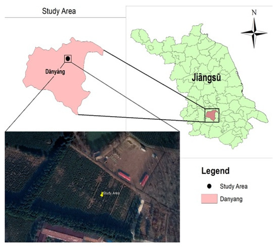
Figure 1.
The study area: a map of Jiangsu province (top right), Danyang district (top left) and an aerial view of the study site (bottom).
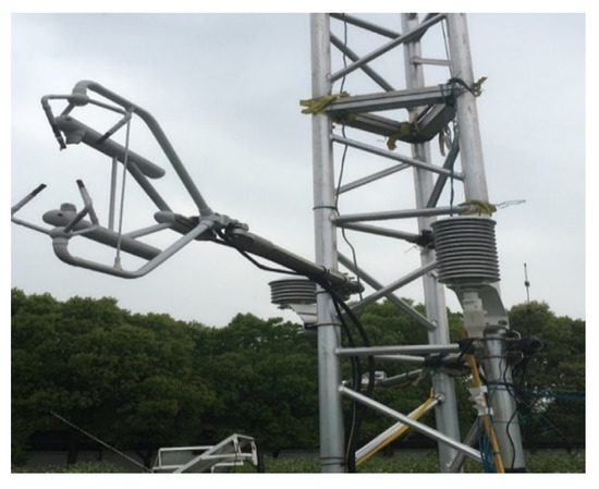
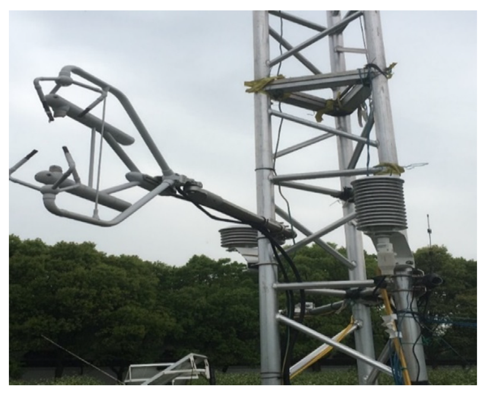
Figure 2.
The eddy covariance system placed on a pole in the study area at the height of 2.3 m.
2.2. Micrometeorological Measurements
A micrometeorological station, with a maximum fetch of 175 m in the direction of the predominant wind, was installed on a 12 m tall aluminum tower in the right corner of the experimental site (Figure 1). This tower was used for supporting all the necessary instrumentation during the experiment. The EC system consisted of a 3-D sonic anemometer to measure the wind speed vector and sonic temperature, and an open-path infra-red gas analyzer that measures the CO2 and H2O concentrations (Figure 2). The sonic anemometer was positioned towards the dominant wind direction to reduce wind distortion effects. The EC raw data were sampled at high frequency (~10 Hz) and half-hourly mean fluxes of sensible and latent heat were recorded on a datalogger (CR-3000) for the whole cropping season, including stable and unstable conditions. Later, the data recorded in the rainy seasons and scattered data were removed and only the data under unstable conditions were considered for the analysis [28,29]. Relative humidity and air temperature were measured using a sensor (HC2S3-L, Campbell Scientific Inc., Logan, UT, USA) placed within a ventilated radiation shield (Figure 2). A net radiometer was mounted at height of 2.3 m above the ground surface on the same pole with the EC system, facing the south direction to avoid the shadowing effect used for measuring the following four components of radiation: incoming and outgoing short wave and longwave radiation, from which the net radiation (Rn) was calculated. Soil heat flux, G, was measured by three soil heat flux plates (TCAV-L, Campbell Scientific Inc., Logan, UT, USA, HFP01, Hukseflux), placed at a depth of 0.08 m within the soil and two miniature thermocouples (type-T) that were placed above each of the heat flux plates at depths of 0.02 m and 0.06 m, respectively. Soil water content (ϴv) was measured by a reflectometer (CS655, Campbell Scientific Inc., Logan, UT, USA). Data collection was performed from November 2018 to July 2019. All the instruments used in the study are given with manufactures names and installation height in Table 1.

Table 1.
Stability conditions based on Monin–Obukhov length [30,31].
2.3. Data Analysis
The change in heat stored above the soil heat flux plates Gstored was determined by Equation (2), which is as follows:
where ρsoil is the soil bulk density, cdsoil is the dry soil specific heat capacity, ρw is the water density, cw is the specific heat capacity of water, ∆z is the soil heat flux plates depth, ∆Tsoil is the average change in the soil temperature above the soil heat flux plate and ∆t is the time between temperature average measurements. The surface soil heat flux was calculated as Equation (3), which is as follows:
For the FV analysis two type T, fine-wire thermocouples of diameter 50-µm were placed near the EC system at a height of 1.8 m above the ground surface, facing the dominant wind direction. The miniature thermocouples were cleaned with acetone (C3H6O), (a cleaning agent) during the visit to the study site for keeping them safe from cobs and insects. All the half-hourly data of the measured variables, including relative humidity, wind speed, air temperature, and wind direction, were stored on an external memory card (16 GB) connected to the datalogger. The raw data from the EC system were processed by Easy-flux data processing software (Campbell Scientific Inc., Logan, UT, USA). Only the data under unstable conditions were used for further analysis and the days with high precipitation were filtered out.
The stability conditions were identified based on theoretical indicators of the stability parameter (ζ), as presented in Table 1, indicating all the available atmospheric conditions. In this study, only unstable data were used for further analysis.
2.4. Fetch and Wind Direction
Before starting the experiment, a field survey was conducted to analyze the dominant wind direction and available fetch. Installing the meteorological tower at the position shown in Figure 1 provided a fetch of 175 m from the field boundary, regarding the predominant wind direction. The EC sensors were installed at 2.3 m height. For a canopy height of 0.8 m, the EC system was at 1.76 m above the zero-plane displacement height. Hence, this installation height met the 100:1 fetch-to-height ratio required for reliable EC measurements.
2.5. Flux Variance Method
The Monion–Obukhov similarity theory (MOST), on which the FV technique is based, describes the correlations between the structure parameters of temperature, relative humidity, and surface fluxes, under the assumption of stationary conditions and horizontal homogeneity [14]. The FV method estimates HFV using standard deviation of the air temperature calculated from high-frequency (~10 Hz) temperature measurements by the fine-wire thermocouples. The sensible heat flux can be expressed as Equation (4).
where ρ is the air density, cp is the air specific heat at constant pressure, σT is standard deviation of air temperature, CT is a similarity constant, z is the measurement height, d is zero-plane displacement, is the mean air temperature and ζ is the atmospheric stability parameter that can be calculated as Equation (5) [32].
where L is the Obukhov length, calculated as Equation (6).
where is the covariance between the vertical velocity and air temperature and is the friction velocity, calculated by Equation (7) [33].
where u′, v′ and w′ are the turbulent fluctuations in the three velocity components.
3. Results and Discussion
3.1. Energy Balance Closure
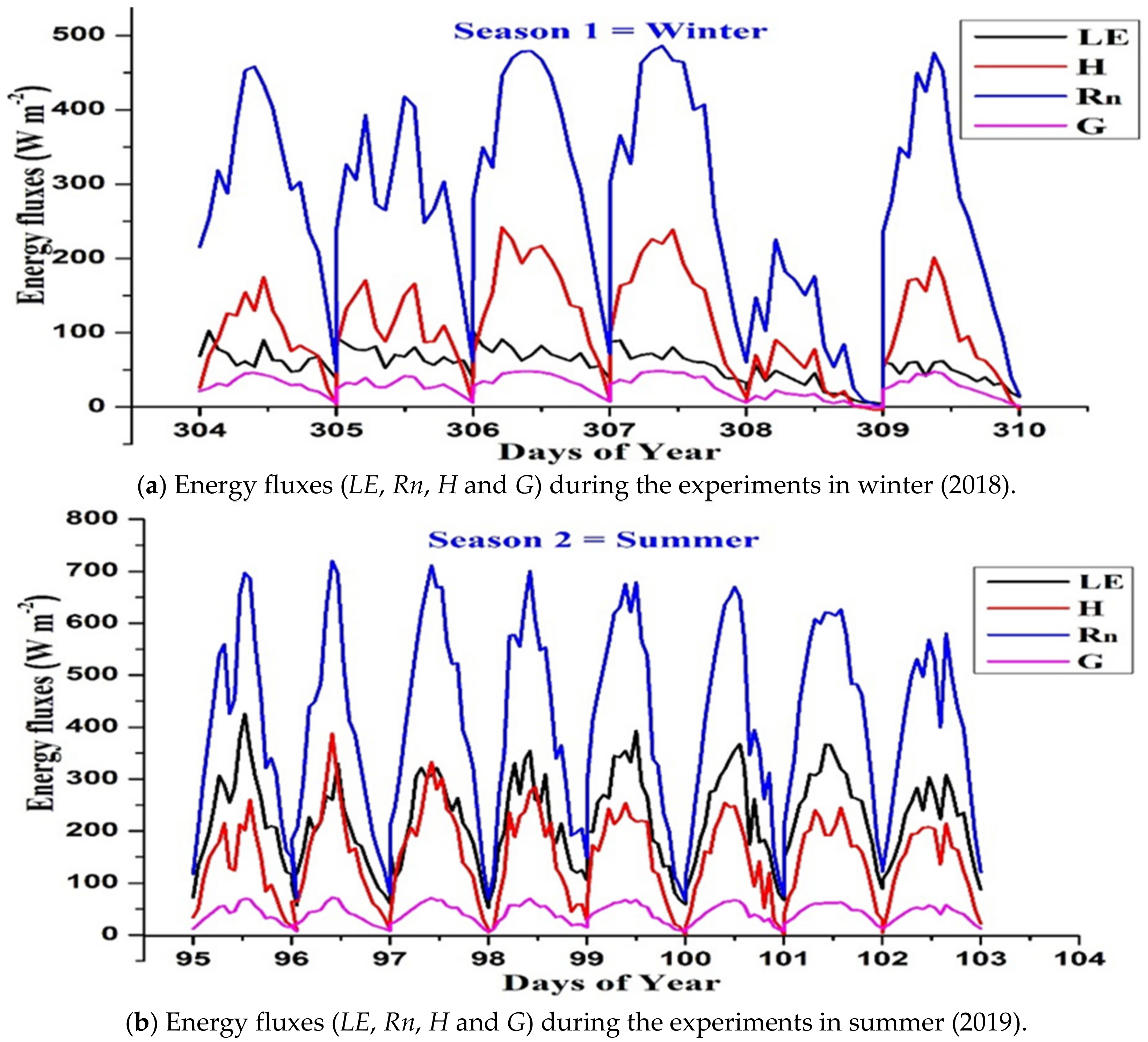
The energy balance closure analysis was performed for evaluating the performance of the EC measurements for two different seasons, Season 1 (winter) and Season 2 (summer). The energy balance analysis was conducted for the whole experimental duration, excluding the stable condition; the stability condition was determined based on the stability coefficient, as expressed in Table 2. Regression analysis was performed between half-hourly datasets of the available energy flux (Rn − G) and the turbulent fluxes of consumed energy (LEEC + HEC) (Figure 3a,b). The available energy flux was relatively high during the summer, with a maximum value of about 700 Wm−2 and was low with a minimum value of about 20 Wm−2. In the winter energy balance, the coefficient of determination was R2 = 0.83, the regression slope was 0.54 and the RMSE was 34.97 Wm−2 (Figure 3a).
Table 2.
Information of the instruments used during the experiment, including manufactures, installation height, notations and measuring units.
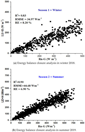
Figure 3.
Energy balance closure analysis: (a) Season 1 in winter (DOY 290–334) 2018; (b) Season 2 in summer (DOY 90–175) 2019.
On the other hand, in summer, the closure demonstrated a relatively high R2 = 0.90, a regression slope of 0.73 and RMSE = 44.68 Wm−2. These results were in line with previous studies and confirm the performance of the eddy covariance system as reported for FLUXNET sites and other eddy covariance applications [34]. In our summer experiment, the surface energy balance closure was within the generally accepted range of 20–30%, an underestimation of the surface fluxes compared to the estimates of available energy [32,33].
Typical diurnal courses of the measured fluxes during the experiment in the summer and winter seasons are presented in Figure 4a,b. The major difference between winter (Figure 4a) and summer (Figure 5) is the relation between sensible and latent heat flux. In winter, LE is significantly lower than H, while in summer, the relation is reversed. The average Bowen ratio, defined as H/LE, during summer was 0.59, while during winter, its value was 1.09. This observation is because summer is rainier; hence, evapotranspiration is higher than sensible heat flux. On the other hand, during the relatively dry winter, most of the net radiation is consumed as sensible heat, which is larger than LE.

Figure 4.
Energy fluxes (LE, Rn, H and G) during the experiments in both seasons. (a) Season 1, winter (2018). (b) Season 2, summer (2019).
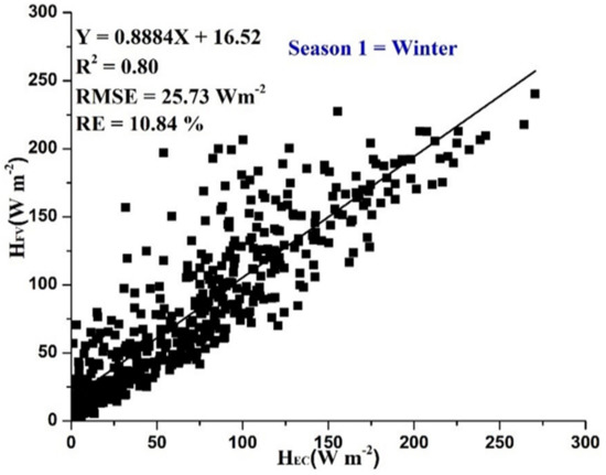
Figure 5.
Regression analysis between the half-hourly dataset of HFV and HEC at the measurement height of 1.8 m for Season 1 (DOY 305–360, 2018).
3.2. Sensible Heat Flux
Regression analysis was performed between the half-hourly data of HFV and HEC. The analysis was performed for unstable conditions only and the days with high precipitation were excluded from further analysis. For the winter season (season 1), the estimated HFV was in good agreement with the HEC with R2 = 0.80, slope of regression of 0.89, RMSE = 25.73 Wm−2 and RE = 10.84%, as shown in Figure 5. The estimation of HFV in Season 2 (summer) was also in reasonable agreement with the HEC with R2 = 0.83, slope of regression of 0.91; the statistical errors of RMSE and RE were 35.49 Wm−2 and 10.5%, respectively, as shown in Figure 6. The estimated HFV was in better agreement with HEC during the summer season, as compared to the winter season. The regression slope for both seasons was reasonable and in agreement with some previous studies, where the slope was also close to unity. RMSE and RE values were in good agreement with several previous studies [10,13,15]. Generally, the FV analysis generated relatively good estimation of HFV as compared with HEC (Table 2).
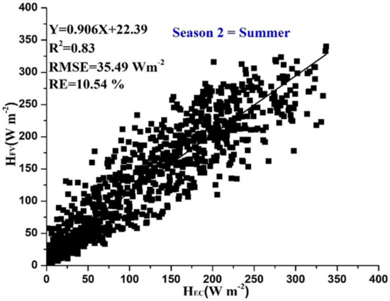
Figure 6.
Regression analysis between the half-hourly dataset of HFV and HEC at the measurement height of 1.8 m for Season 2 (summer, DOY 60–210, 2019).
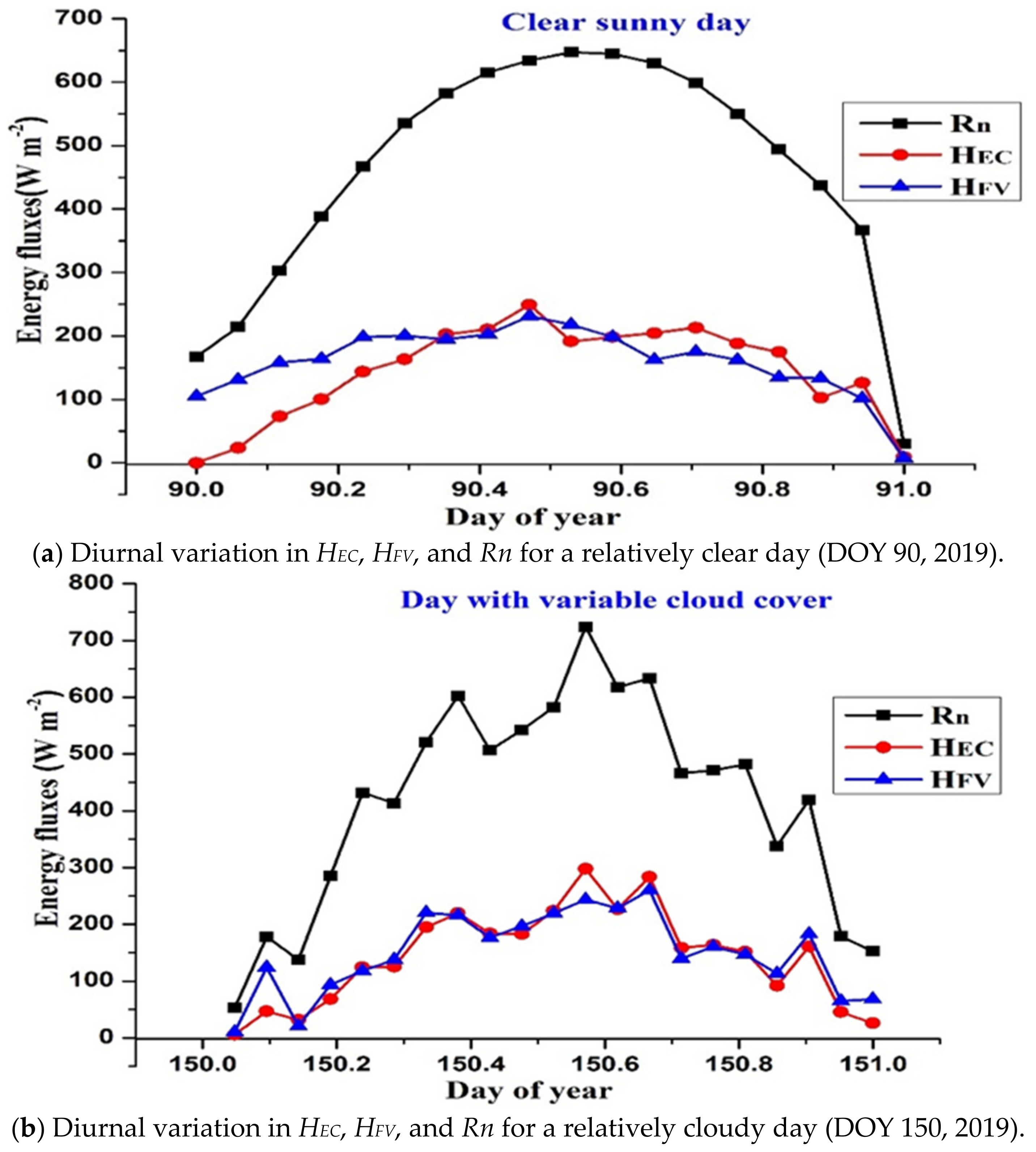
The diurnal variations in the estimated H from both FV and EC methods are presented for two different days, a clear sunny day (DOY 90, Figure 7a) and a day with partial cloud cover (DOY 150, Figure 7b). The curves suggest that HFV and HEC demonstrated better correlation during the day with variable cloudiness (Figure 7b, DOY 150, 2019) than on the clear day (Figure 7a, DOY 90). On the other hand, the estimations of the HFV and HEC were in better agreement mainly at midday; in spite of the good agreement, the HFV and HEC fluctuated with the change in Rn. On the clear day (DOY 90, 2018), a more consistent increase in the Rn was observed throughout the day (Figure 7a).
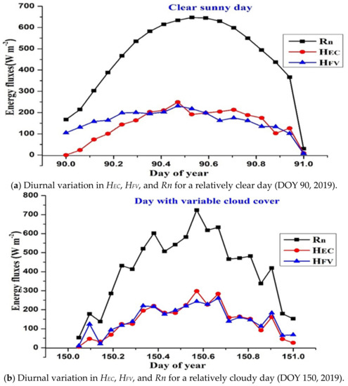
Figure 7.
Diurnal variation in the half-hourly dataset of HEC and HFV, along with the Rn for (a) a clear day (DOY 90, 2019) and (b) day with variable cloudiness (DOY (150, 2019).
3.3. Latent Heat Flux
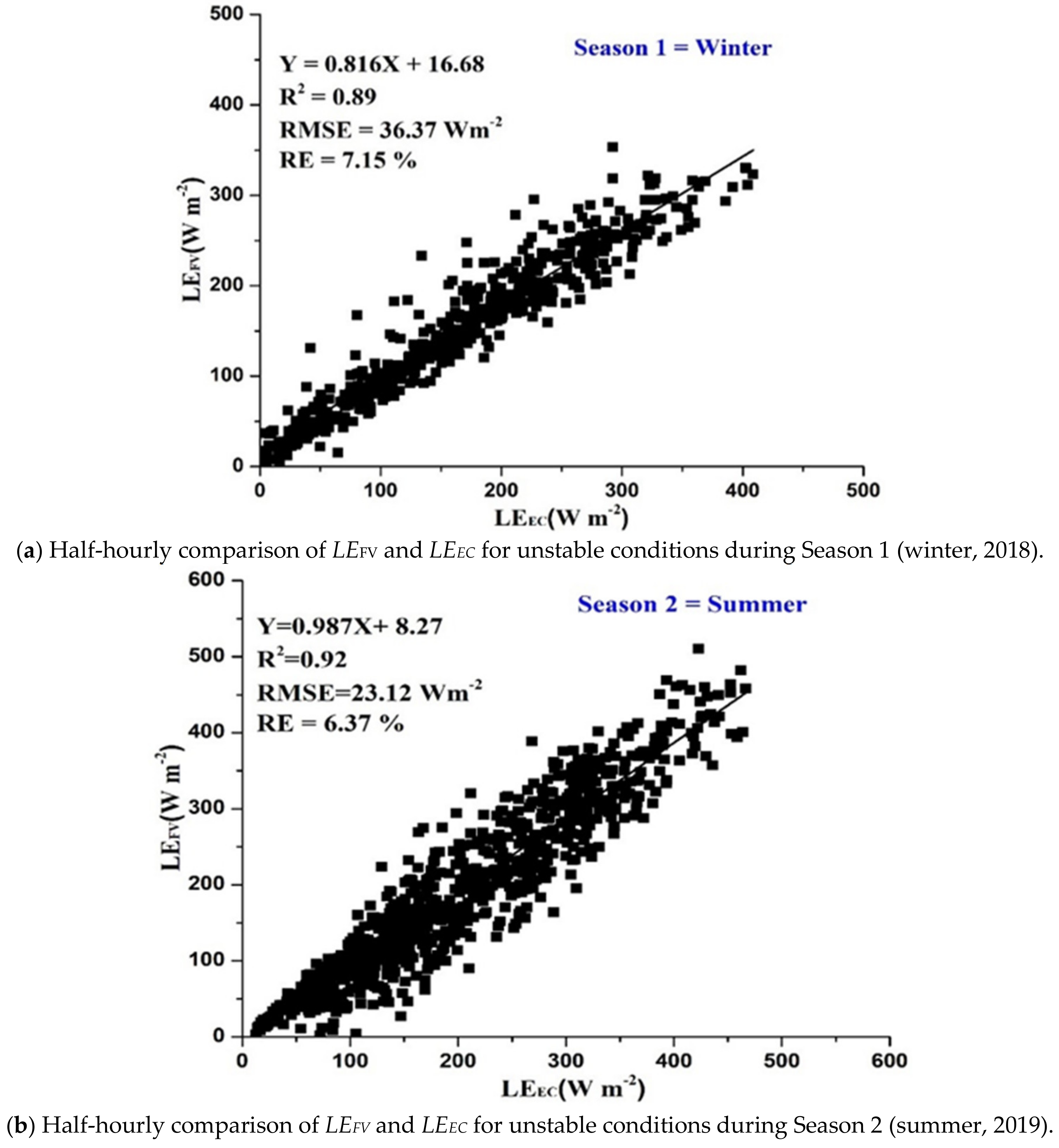
The latent heat flux was extracted as a residual of the energy balance closure, with HFV along with Rn and G measured separately. The half-hourly estimates of the LEFV were regressed against the half-hourly measurements of LEEC, during the two different seasons, winter (2018) and summer (2019). The half-hourly regression between the LEFV and LEEC during the winter demonstrated R2 = 0.89, a regression slope of 0.82 and RMSE = 36.37 Wm−2. The estimated mean value of the LEFV was relatively low in the winter, with a value of 150 Wm−2 (Figure 8a). During the summer of 2019, the half-hourly regression analysis between the LEFV and LEEC resulted in R2 = 0.93, a slope of regression of 0.99 and RMSE = 23.12 Wm−2. The LE was relatively high in summer, with a mean value of about 450 Wm−2. Overall, the FV estimates were in good agreement against the eddy covariance (Table 3).

Figure 8.
Comparison of estimated latent heat flux against the measurements of the eddy covariance system during two seasons. (a) Half-hourly comparison of LEFV and LEEC for unstable conditions during Season 1 (winter, 2018). (b) Half-hourly comparison of LEFV and LEEC for unstable conditions during Season 2 (summer, 2019).
Table 3.
Regression statistics of half-hourly estimations of the FV and EC system.
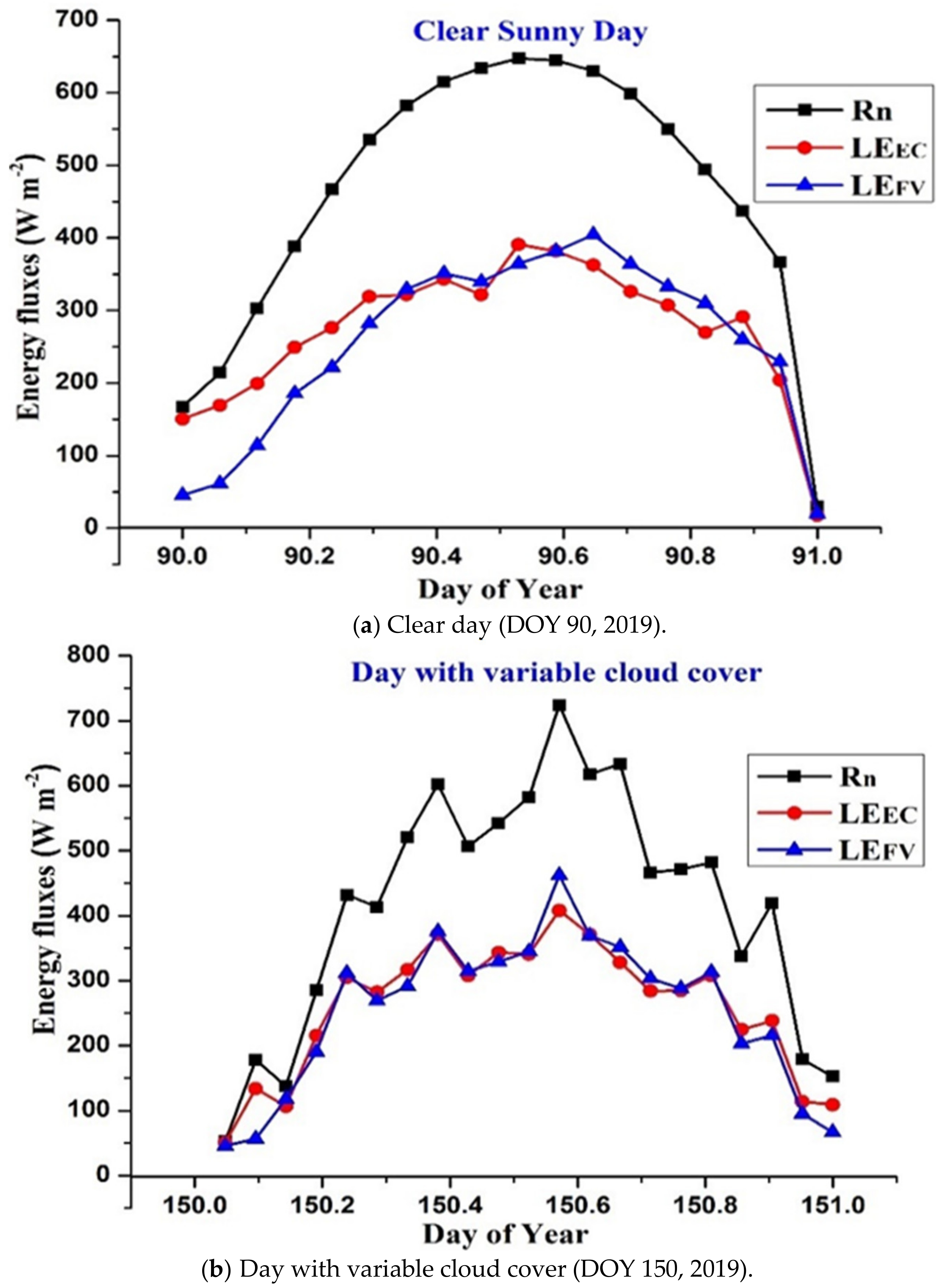
Diurnal variation in the half-hourly datasets of the LEFV and LEEC, along with Rn, was used for evaluating the performance of the FV method for the estimation of the LE during two different days, one with clear sky and another with variable cloudiness. On the clear day, the LEFV was overestimated in the latter part of the day (evening), and LEEC was larger than LEFV in the morning (Figure 9a). During the cloudy day, LE estimations by both EC and FV closely followed the diurnal variation in Rn (Figure 9b).
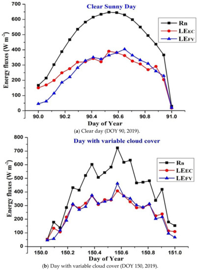
Figure 9.
Diurnal variations in the LEEC and LEFV, along with the net radiation, for two different days: (a) clear day (DOY 90, 2019); (b) day with variable cloud cover (DOY 150, 2019).
3.4. Seasonal Estimates of the Energy Balance Components
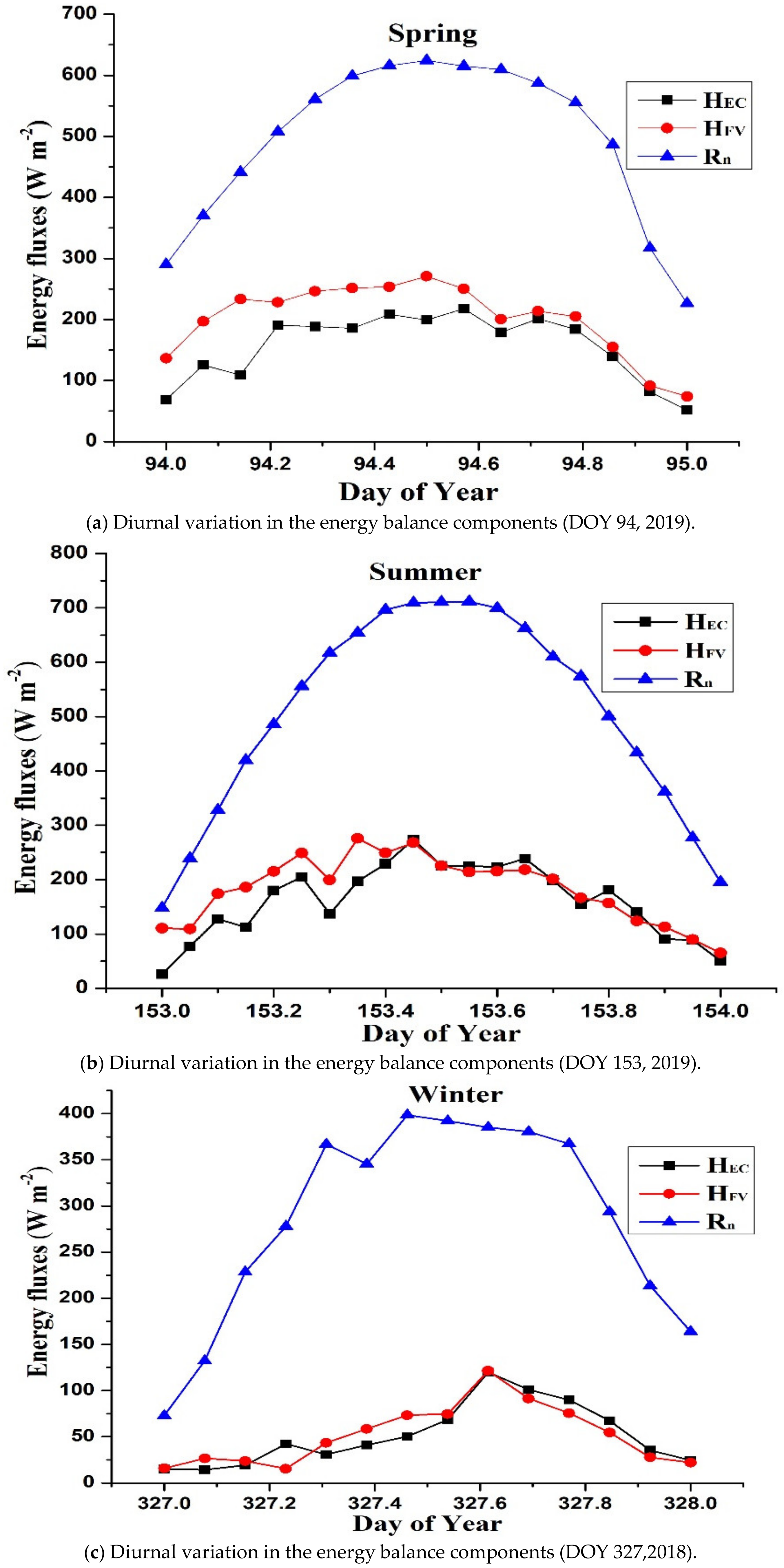
The diurnal estimates of the turbulent fluxes were obtained by summing the half-hourly estimates during unstable conditions. The daily total Rn was constant throughout the winter, gradually climbed to its highest value during the summer, and then decreased to its minimum value at the start of the winter, as observed in (Figure 10b). In summer, one random clear day was selected without clouds (DOY 153); the Rn was very smooth throughout the day, with the highest value of over 700 Wm−2.
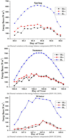
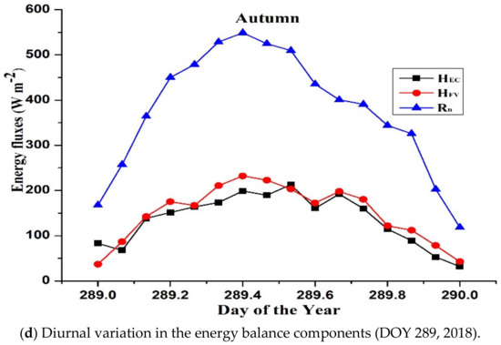
Figure 10.
Diurnal variation in net radiation and sensible heat flux estimated by the FV, and EC methods during different climatic conditions (a–d), representing different seasons during 2018-2019.
The FV overestimated the H in the morning and it was close to the measurements of the EC system in the evening (Figure 10b). In winter, daily Rn was very low, with a peak value ranging from 300 to 400 Wm−2 for most of the days. A random day was selected during the winter for representation of the analysis, including the estimations of the H from the FV, and EC methods (Figure 10c). The majority of Rn was utilized as H during the dry times and as LE following the rainy episodes. Variability in the Rn, due to clouds affecting solar radiation, impacts on the available energy. Variability in the H and LE from day to day and season to season were mainly ascribed to the rain events and Rn influences on the available energy. After the end of the spring, the LE magnitude increased significantly, peaked in the middle of the summer, and then significantly declined to its minimum value in the winter; the daily LE estimations were below 100 Wm−2 in winter, primarily because Rn was lower. Consequently, the H used up more of the available energy, due to increased Rn and LE reached its maximum in the summer at 300 Wm−2, making it the main factor in the energy balance equation. The magnitude of the G changed with the change in net radiation; as the G decreased, more energy was available for distribution between the LE and H. Generally, the estimates of the H and LE obtained for the FV method were more compatible during the summer and spring.
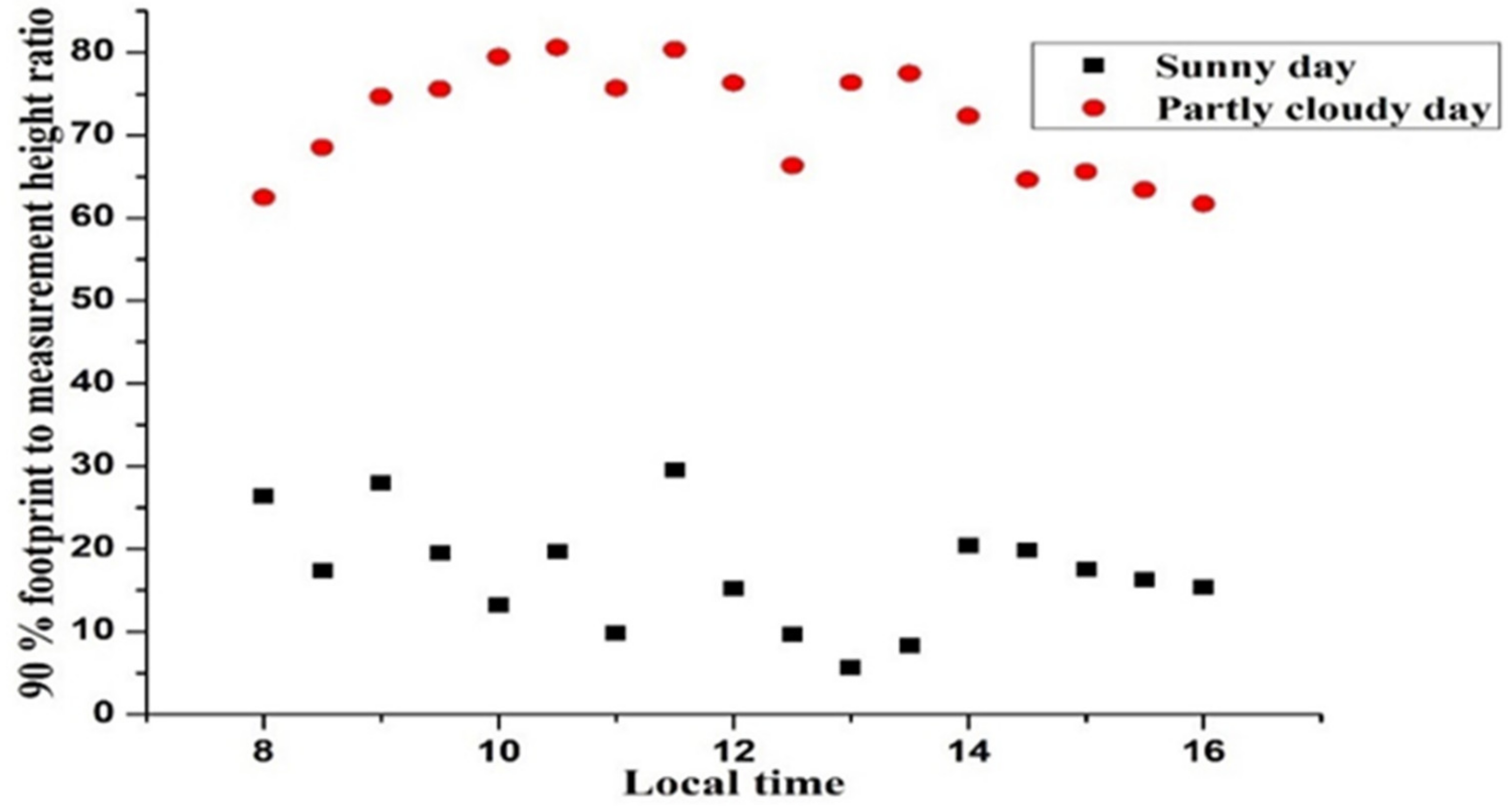
3.5. Footprint Analysis of the EC System
Since the footprint establishes the relative influence of the underlying surface area on the measured fluxes, it is essential to estimate the footprint for the sensible heat flux in agricultural and environmental investigations. The proportional contribution of the windward distance to the surface fluxes detected by the EC system was examined using a footprint model [35]. The ratio of the measurement height to the 90% flux footprint distance for unstable conditions was calculated using the footprint model [27]. Two days from the trail period were chosen, each with different climatic conditions, including one (1 June 2019) cloudy day and one (23 March 2019) cloudy to sunny day. Figure 11 illustrates the daily variation in footprint/height ratio for these days. The ratio throughout the sunny day was in the range of 0 to 30, according to the results in Figure 11, which was notably lower than the ratio and varied between 50 to 80 on the cloudy day. The surface was warmer and the boundary layer was more unstable on the bright day than it was on the overcast day, which accounts for the discrepancy. Due to this greater instability, the 90% flux footprint extended further on sunny days than on cloudy ones [36]. Additionally, Figure 11 demonstrates that on both days, the ratio is lower than the typical fetch/height ration of 100:1. The findings suggests that the majority of the flux measured by the EC system during the experiment came from the tea field under investigation. As a result, the EC data are trustworthy and may be used to compare the FV technique.
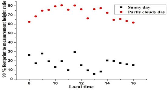
Figure 11.
Variation in half-hourly 90% footprint to measurement height ratio for two days, one cloudy day (1 June 2019) and the other cloudy to sunny day (23 March 2019).
4. Discussion
In this study, the performance of the FV method for the long-term estimation of surface fluxes, including H and LE in the open field, was conducted for the first time in the tea field. The results showed that the FV method was effective for the estimation of surface fluxes and provided precise estimations of latent heat flux. The regression between HFV and the HEC for the whole cropping season, including different climatic conditions, was studied. Overall, the results suggested that the estimation of HFV was in good agreement in the summer season, as compared to the other three seasons, due to the clear sky. Zhao et al., (2010) performed experiments using the SR and FV methods on two different agricultural sites in rice paddy and wheat fields, under different climatic conditions; the estimation of HFV was in good agreement against the eddy covariance HEC. The RMSE from the SR analysis was less than that of the FV method [37]. Castellvi et al., (2005) conducted experiments for the estimation of the SR and FV methods, over a heterogeneous canopy in semi-arid climatic conditions. The results showed the performance of the SR method was better compared to the FV method in unstable conditions [38]. Wang et al., (2013) carried out experiments for the estimation of the surface fluxes using the FV method over homogeneous, open and flat grassland in the eastern Tibetan Plateau, which was studied in the hot season under typical humid conditions and during the rainy season, using the EC measurements and the FV methods. The results showed that heat was transported better than water vapor and CO2. The data used in this study were mostly from the hot season under common humid conditions and during the rainy season; these are only estimated for the summer and hydrological conditions, but not applied for the other seasons [17]. Guo et al., (2009) tested the FV technique through experiments using the EC method for the estimation of the LE and CO2 fluxes under unstable conditions. It was concluded that in the absence of the turbulence observations of windy velocity, the FV method can be used to fill flux gaps. The majority of the HFV values deviated from 15 Wm−2; HEC was estimated as less than 20% [39]. Tanny et al., (2016) estimated the surface fluxes in the screen houses over paper using the FV technique and the results of the FV estimations were compared against the EC method. The FV method was in good agreement with the estimations of the EC method at a relatively low cost [40]. Ahiman et al., (2018) conducted experiments to verify the applicability of the FV method over three different agricultural fields; in this study, the application of the FV method was tested and calibrated against the EC method in three different fields. The results showed that the FV technique was appropriate and reliable for the first field (S1) for measurements and calibration; on the other hand, the results in the S3 were not good [41]. Thus, the FV method was proven as a very good candidate for the monitoring of the surface fluxes at a relatively low cost as compared to the eddy covariance method, due to its low cost, simplicity, and simple instrumentation. The FV method has the advantage over other micrometeorological methods, since it requires only the measurements of scalar of interest at one point. The FV method can offer relatively simple, low-cost and accurate estimations of the sensible heat flux. These methods have been applied over different surface and climatic conditions at relatively low costs. The FV technique is a compelling contender for growers to utilize the daily estimates of the LE as a tool for managing irrigation. In this study, two major concerns regarding the application of the FV method were resolved, including the application of the FV method at the farm level, and the robustness of the thermocouple was justified for the long-term estimations. Second, we attempted to verify the acceptability of the FV method for the whole cropping season; the main benefit of such a long-term study was to examine the performance under different climatic conditions, which was studied successfully for the tea crop. Although, there are still some limitations that exist in the application of the FV method. Therefore, future research on the application of the FV method should concentrate on how to use it to calculate scalar fluxes of carbon dioxide, water vapors and other fluxes. Additionally, the method used in the study does not permit real-time estimation of the sensible heat flux; therefore, additional experiments on this topic would be worthwhile.
5. Conclusions
The efficacy of the FV method was assessed for the long-term estimation of the H and LE under unstable conditions in tea plants for the whole cropping season, including winter, summer, autumn and spring. The results were contrasted with those from the EC system. Overall, the estimation of the HFV was in good agreement with the EC in both seasons, as both coefficients of determination were higher than 0.8, and the slope of regression was close to unity. The best result of HFV was observed in summer, with a relatively high R2 of 0.91. The estimated HFV reported a relatively good LEFV in summer; regression of LEFV against LEEC resulted in an R2 of 0.89. Hence, the FV method produced reliable results, regardless of seasonal variations, and most of the estimations were in reasonable agreement with the eddy covariance system. Based on the findings, the FV method offers a simplified and relatively inexpensive method for the estimation of sensible and latent heat fluxes of Camellia sinensis.
Author Contributions
Conceptualization, N.A.B. and Y.H.; methodology, N.A.B.; software, A.R.; validation, J.T., F.A. and M.I.K.; writing—original draft preparation, N.A.B.; writing—review and editing, J.T.; visualization, A.S.; supervision, Y.H.; funding acquisition, Y.H. and M.B.I.; resources, Y.N. and A.S.; data curation, N.S.; investigation, A.A. All authors have read and agreed to the published version of the manuscript.
Funding
The authors are grateful to the financial support by the Key R & D Program of Jiangsu Provincial Government (BE2021340) and the Priority Academic Program Development of Jiangsu Higher Education Institutions (PAPD-2018-37).
Institutional Review Board Statement
Not applicable.
Informed Consent Statement
Not applicable.
Conflicts of Interest
The authors declare no conflict of interest.
References
- Gowda, P.H.; Chávez, J.L.; Colaizzi, P.D.; Evett, S.R.; Howell, T.A.; Tolk, J.A. ET mapping for agricultural water management: Present status and challenges. Irrig. Sci. 2008, 26, 223–237. [Google Scholar] [CrossRef]
- Rosset, M.; Riedo, M.; Grub, A.; Geissmann, M.; Fuhrer, J. Seasonal variation in radiation and energy balances of permanent pastures at different altitudes. Agric Meteorol. 1997, 86, 245–258. [Google Scholar] [CrossRef]
- Wever, L.A.; Flanagan, L.B.; Carlson, P.J. Seasonal and interannual variation in evapotranspiration, energy balance and surface conductance in a northern temperate grassland. Agric. For. Meteorol. 2002, 112, 31–49. [Google Scholar] [CrossRef]
- Tha, P.U.K.; Jie, Q.; Hong-Bing, S.; Tomonori, W.; Yves, B. Surface renewal analysis: A new method to obtain scalar fluxes. Agric Meteorol. 1995, 74, 119–137. Available online: https://www.sciencedirect.com/science/article/pii/016819239402182J (accessed on 22 June 2019).
- Czikowsky, M.J.; Fitzjarrald, D.R. Evidence of seasonal changes in evapotranspiration in eastern U.S. hydrological records. J. Hydrometeorol. 2004, 5, 974–988. [Google Scholar] [CrossRef]
- Drexler, J.Z.; Snyder, R.L.; Spano, D.; Paw, U.K.T. A review of models and micrometeorological methods used to estimate wetland evapotranspiration. Hydrol. Proc. 2004, 18, 2071–2101. [Google Scholar] [CrossRef]
- RAllen, G.; Pereira, L.S.; Howell, T.A.; Jensen, M.E. Evapotranspiration information reporting: I. Factors governing measurement accuracy. Agric Water Manag. 2011, 98, 899–920. [Google Scholar]
- Buttar, N.A.; Yongguang, H.; Shabbir, A.; Lakhiar, I.A.; Ullah, I.; Ali, A.; Aleem, M.; Yasin, M.A. Estimation of evapotranspiration using Bowen ratio method. IFAC PapersOnLine 2018, 51, 807–810. [Google Scholar] [CrossRef]
- Wang, J.; Raza, A.; Hu, Y.; Buttar, N.A.; Shoaib, M.; Saber, K.; Li, P.; Elbeltagi, A.; Ray, R.L. Development of Monthly Reference Evapotranspiration Machine Learning Models and Mapping of Pakistan—A Comparative Study. Water 2022, 14, 1666. [Google Scholar] [CrossRef]
- Sunmonu, L.A.; Olufemi, A.P.; Abiye, O.E.; Babatunde, O.A. Estimation of sensible heat flux at a tropical location: A performance evaluation of half-order time derivative method. Model. Earth Syst. Environ. 2019, 5, 1215–1220. [Google Scholar] [CrossRef]
- Nile, E. Sensible Heat Flux under Unstable Conditions for Sugarcane Using Temperature Variance and Surface Renewal. 2010. Available online: https://ukzn-dspace.ukzn.ac.za/handle/10413/600 (accessed on 11 May 2019).
- Hu, Y.; Buttar, N.A.; Tanny, J.; Snyder, R.L.; Savage, M.; Lakhiar, I.A. Surface renewal application for estimating evapotranspiration: A review. Adv. Meteorol. 2018, 2018, 1690714. [Google Scholar] [CrossRef]
- Jizhang, W.; Buttar, N.A.; Yongguang, H.; Lakhiar, I.A.; Javed, Q.; Shabbir, A. Estimation of sensible and latent heat fluxes using surface renewal method: Case study of a tea plantation. Agronomy 2021, 11, 179. [Google Scholar] [CrossRef]
- Tillman, J.E. The indirect determination of stability, heat and momentum fluxes in the atmospheric boundary layer from simple scalar variables during dry unstable conditions. J. Appl. Meteorol. 1972, 11, 783–792. [Google Scholar] [CrossRef]
- Castellví, F.; Buttar, N.A.; Hu, Y.; Ikram, K. Sensible heat and latent heat flux estimates in a tall and dense forest canopy under unstable conditions. Atmosphere 2022, 13, 264. [Google Scholar] [CrossRef]
- Castellvi, F.; Martínez-Cob, A. Estimating sensible heat flux using surface renewal analysis and the flux variance method: A case study over olive trees at Sástago (NE of Spain). Water Resour. Res. 2005, 41, 1–10. [Google Scholar] [CrossRef]
- Shaoying, W.; Yu, Z.; Shihua, L.; Heping, L.; Lunyu, S. Estimation of turbulent fluxes using the flux-variance method over an alpine meadow surface in the eastern Tibetan Plateau. Adv. Atmos Sci. 2013, 30, 411–424. [Google Scholar]
- Haymann, N.; Lukyanov, V.; Tanny, J. Effects of variable fetch and footprint on surface renewal measurements of sensible and latent heat fluxes in cotton. Agric. For. Meteorol. 2019, 268, 63–73. [Google Scholar] [CrossRef]
- Chor, T.L.; Dias, N.L.; Araújo, A.; Wolff, S.; Zahn, E.; Manzi, A.; Trebs, I.; Sá, M.O.; Teixeira, P.R.; Sörgel, M. Flux-variance and flux-gradient relationships in the roughness sublayer over the Amazon forest. Agric. For. Meteorol. 2017, 239, 213–222. [Google Scholar] [CrossRef]
- Ahiman, O.; Mekhmandarov, Y.; Pirkner, M.; Tanny, J. Application of the flux-variance technique for evapotranspiration estimates in three types of agricultural structures. Int. J. Agron. 2018, 2018, 7935140. [Google Scholar] [CrossRef]
- Buttar, N.A.A.M.; Yongguang, H.; Chuan, Z.; Tanny, J.; Ullah, I. Height effect of air temperature measurement on sensible heat flux estimation using flux variance method. Pak. J. Agric. Sci. 2019, 56, 793–800. [Google Scholar]
- De Bruin, H.A.R.; Kohsiek, W.; Van Den Hurk, B.J.J.M. A verification of some methods to determine the fluxes of momentum, sensible heat, and water vapour using standard deviation and structure parameter of scalar meteorological quantities. Bound. Layer Meteorol. 1993, 63, 231–257. [Google Scholar] [CrossRef]
- Padro, J. An investigation of flux-variance methods and universal functions applied to three land-use types in unstable conditions. Bound. Layer Meteorol. 1993, 66, 413–425. [Google Scholar] [CrossRef]
- Albertson, J.D.; Parlange, M.B.; Katul, G.G.; Chu, C.-R.; Stricker, H.; Tyler, S. Sensible heat flux from arid regions: A simple flux-variance method. Water Resour. Res. 1995, 31, 969–973. [Google Scholar] [CrossRef]
- Gao, Z.; Bian, L.; Chen, Z.; Sparrow, M.; Zhang, J. Turbulent variance characteristics of temperature and humidity over a non-uniform land surface for an agricultural ecosystem in China. Adv. Atmos. Sci. 2006, 23, 365–374. [Google Scholar] [CrossRef]
- Kaimal, J.; Finnigan, J. Atmospheric Boundary Layer Flows: Their Structure and Measurement; Oxford University Press: New York, NY, USA, 1994. [Google Scholar]
- Wilczak, J.M.; Oncley, S.P.; Stage, S.A. Sonic anemometer tilt correction algorithms. Bound. Layer Meteorol. 2001, 99, 127–150. [Google Scholar] [CrossRef]
- Buttar, N.A.; Yongguang, H.; Tanny, J.; Akram, M.W.; Shabbir, A. Fetch effect on flux-variance estimations of sensible and latent heat fluxes of camellia sinensis. Atmosphere 2019, 10, 299. [Google Scholar] [CrossRef]
- Stull, R.B. Transilient turbulence theory. The concept of eddy-mixing across finite distances—1. J. Atmos. Sci. 1984, 41, 3351–3367. [Google Scholar] [CrossRef]
- Garratt, J.R. Review: The atmospheric boundary layer. Earth-Sci. Rev. 1994, 37, 89–134. [Google Scholar] [CrossRef]
- Wilson, A.K.; Goldstein, A.; Falge, E.; Aubinet, M.; Baldocchi, D.; Berbigier, P.; Bernhofer, C.; Ceulemans, R.; Dolman, H.; Field, C.; et al. Energy balance closure at FLUXNET sites. Agric. Meteorol. 2002, 113, 223–243. [Google Scholar]
- Yuling, F. Energy balance closure at ChinaFLUX sites. Sci. China Earth Sci. 2005, 48, 51–62. [Google Scholar]
- Renhua, Z. Determination of Averaging Period Parameter and Its Effects Analysis for Eddy Covariance Measurements. Sci. China Ser. D Earth Sci. 2005, 48, 33–41. [Google Scholar]
- Nitai, H.; Lukyanov, V.; Cohen, S.; Tanny, J. Effect of variable fetch on surface renewal estimates of sensible and latent heat fluxes in cotton. In Proceedings of the 20th EGU General Assembly, EGU2018, Vienna, Austria, 4–13 April 2018; p. 12561. [Google Scholar]
- Hsieh, C.-I.; Katul, G.; Chi, T.-W. An approximate analytical model for footprint estimation of scalar fluxes in thermally stratified atmospheric flows. Adv. Water Resour. 2000, 23, 765–772. [Google Scholar] [CrossRef]
- Savage, M.J.; Everson, C.S.; Odhiambo, G.O.; Mengistu, M.G.; Jarmain, C. Theory and Practice of Evaporation Measurement, with Spatial Focus on SLS as an Operational Tool for the Estimation of Spatially-Averaged Evaporation; Report No. 1335/1/04; Water Research Commission: Pretoria, South Africa, 2004; p. 204. ISBN 1-77005-247-X.
- Zhao, X.; Liu, Y.; Tanaka, H.; Hiyama, T. A comparison of flux variance and surface renewal methods with eddy covariance. IEEE J. Sel. Top. Appl. Earth Obs. Remote Sens. 2010, 3, 345–350. [Google Scholar] [CrossRef]
- Castellví, F. An advanced method based on surface renewal theory to estimate the friction velocity and the surface heat flux. Water Resour. Res. 2018, 54, 10134–10154. [Google Scholar] [CrossRef]
- Guo, X.; Zhang, H.; Cai, X.; Kang, L.; Zhu, T.; Leclerc, M.Y. Flux-variance method for latent heat and carbon dioxide fluxes in unstable conditions. Bound. Layer Meteorol. 2009, 131, 363–384. [Google Scholar] [CrossRef]
- Mekhmandarov, Y.; Pirkner, M.; Achiman, O.; Tanny, J. Application of the surface renewal technique in two types of screenhouses: Sensible heat flux estimates and turbulence characteristics. Agric. For. Meteorol. 2015, 203, 229–242. [Google Scholar] [CrossRef]
- Tanny, J.; Achiman, O.; Mazliach, Y.; Lukyanov, V.; Cohen, S.; Cohen, Y. The effect of variable fetch on flux-variance estimates of sensible and latent heat fluxes in a pepper screenhouse. Acta Hortic. 2016, 1197, 109–116. [Google Scholar] [CrossRef]


Publisher’s Note: MDPI stays neutral with regard to jurisdictional claims in published maps and institutional affiliations. |
© 2022 by the authors. Licensee MDPI, Basel, Switzerland. This article is an open access article distributed under the terms and conditions of the Creative Commons Attribution (CC BY) license (https://creativecommons.org/licenses/by/4.0/).