Abstract
Constructing accurate models that provide information about water vapor content in the troposphere improves the reliability of numerical weather forecasts and the position accuracy of low-cost Global Navigation Satellite System (GNSS) receivers. However, developing models with high spatial-temporal resolution demands compact observational datasets in the regions of interest. Empirical models, such as the Global Pressure and Temperature 3 (GPT3w), have been constructed based on the monthly averaged outputs of numerical weather models. These models are based on the assimilation of existing measurements to provide estimations of atmospheric parameters. Therefore, their accuracy may be reduced over regions with a low resolution of radiosonde or continuous GNSS stations. By emerging and increasing the Low-Earth-Orbiting (LEO) satellites that measure atmospheric parameter profiles using the Radio Occultation (RO) technique, new opportunities have appeared to acquire high-resolution atmospheric observations at different altitudes. This study aims to apply these RO observations to improve the accuracy of the GPT3w model over Iran, which is sparse in terms of long-term GNSS and radiosonde measurements. The temperature, pressure, and water vapor pressure parameters from the GPT3w model have been used as the input layers of the Extremely Learning Machine (ELM) technique. The wet refractivity indices from the RO technique are considered target parameters in the output layer to train the ELM. The RO observations of 2007–2020 are applied for training, and those of 2020–2022 for evaluating the performance of the developed ELM. Our numerical results indicate that the developed ELM decreases the Root-Mean-Square Error (RMSE) values of the wet refractivity indices by about 17 percent, compared to the original GPT3w RMSE values. Additionally, the wet refractivity indices from ELM have revealed correlation coefficients of about 0.64, which is about 1.9 times those related to the original GPT3w model. The performance of ELM has also been examined by comparison with the data of six located radiosonde stations covering the year 2020. This comparison shows an improvement of about 14 percent in the average RMSE values of the estimated wet refractivity indices.
1. Introduction
The water vapor content or wet refractivity indices information from atmospheric models can be applied to investigate climate change [1], predicting storm hazards or rainfall [2]. This parameter can be obtained from measurements of the in situ meteorological instruments (e.g., radiosonde stations) [3], the atmospheric tomography method using space-based observations [4,5,6], or existing atmospheric models [7,8]. Wet refractivity indices are based on water vapor pressure and temperature and reveal numerous local features due to severe weather variability [4]. Therefore, a dataset with high spatial-temporal resolution is required to construct the atmospheric models to be able to represent the local fluctuations in the weather-related parameters and to improve their accuracy. Observations of the radiosonde balloons, used for measuring temperature and humidity, are the main inputs for calculating the wet refractivity indices at different altitudes. However, due to the expensive cost and the high operational demands, the temporal and spatial resolution of these observations is limited [9]. Tomography approaches are complementary techniques, which demand high-quality input measurements, such as those of dense GNSS networks. They also require a meticulous mathematical framework to account for limitations, such as the need for and regularization to compensate for the ill condition of these models [10]. For example, Forootan et al. 2019 [4] applied a functional tomography approach to overcome this problem, showing that the retrieved wet refractivity indices can be estimated with the mean Root-Mean-Square Error (RMSE) of about 1.9 ppm, which was 22% better than that related to the corresponding numerical model values. Other examples of the tomography research can be found in [6,10,11,12].
Atmospheric parameters can also be obtained from models that are constructed based on the assimilation of different atmospheric observations into physics-based models, such as ERA5 [13], ERA-Interim [14], or the Global Forecast System (GFS) [15]. Other choices are the empirical models constructed based on the temporally averaged data from the forecasting or reanalysis models (e.g., ERA-Interim) [7]. For example, the University of New Brunswick (UNB) proposed the UNB atmospheric model series that could provide atmospheric parameters with a resolution of about 15 degrees in the latitude direction. From these series, the UNB3 model was proposed by Collins and Langley (1997) to accomplish this estimation with higher accuracy. However, this series of atmospheric models could not represent the zonal changes in the atmospheric parameters (the longitude direction changes had not been considered). Furthermore, due to their low spatial resolution, they are found to be contaminated by considerable errors in some areas [16]. From the Global Pressure and Temperature (GPT) series atmospheric models [17], the GPT2 is codeveloped by Lagler et al. (2013) [18], based on 10 years of monthly averaged atmospheric parameters of the ERA-Interim model [7]. This model represents changes in the atmospheric parameters in both the horizontal and vertical directions with a spatial resolution of about 5 degrees.
To further improve the resolution and to provide more atmospheric parameters, the GPT2w model was introduced by Böhm et al. 2015 [7]. The resolution of this model was about one degree and provided the weighted mean temperature and the water vapor lapse rate as outputs. By using the GPT2w model, hydrostatic and wet tropospheric delays with elevation angles up to 3 degrees can be calculated. Comparing the GPT2w-derived Zenith Total Delay (ZTD) with 341 globally distributed stations shows about 1 mm and 3.6 cm in the values of mean bias and Standard Deviation (STD), respectively [7]. The latest version of GPT (i.e., GPT3w) [19] can be used to calculate geodetic, meteorological, and climatological parameters, such as temperature, pressure, water vapor pressure, wet mapping coefficients, and hydrostatic and wet atmospheric gradient coefficients.
Empirical models are often more favourable for low-cost positioning applications. However, their accuracy is limited due to the usage of temporally averaged data for estimating atmospheric parameters. The accuracy and reliability of these models can be improved by the infusion of new observations, where the GNSS-derived Zenith Wet delay (ZWD) or radiosonde stations data can provide such observations [16]. However, some regions are not well covered by these measurements or the access to these data is limited.
The Radio Occultation (RO) technique provides an opportunity to measure atmospheric parameters on the global scale [20]. These observations provide wet refractivity indices at different altitudes and are widely used to improve the retrieving accuracy of atmospheric parameters [21,22], or they are assimilated into numerical atmospheric models (e.g., in ERA5) [20]. Xia et al. 2013 [23] used RO observations in a two-step reconstruction technique for an atmosphere tomography problem and showed around 14 percent improvement in the accuracy of estimated water vapor. Therefore, RO data are applied in this study to provide new observations in a data-sparse region such as Iran, where only a limited number (e.g., six radiosonde stations) of permanent radiosonde stations exist [24].
Artificial Neural Network (ANN) techniques have been used to improve the accuracy of empirical models [16,25,26]. This method has the capability of learning the structure of non-linear processes by constructing neuron-based mathematical models [27]. Yang et al. 2021 [16] utilized ANN to improve the GPT3-derived Zenith Total Delay (ZTD) via a local GNSS network, where GNSS ZTD values were applied as input of ANN. The results of this study demonstrated improvements of about 37 to 52 percent in the derived ZTD values.
For applying the ANN methods, often supervised learning algorithms with iterative back-projection are used to estimate weights and biases [28]. However, this learning method has the disadvantage of low convergence time, and its solution may be trapped in local minimums [29]. To eliminate these problems, Huang et al. 2006 [30] proposed the Extremely Learning Machine (ELM) method, which is a neural network with a single hidden layer, where the weight and bias of neurons are estimated using the Least Squares (LS) method. Since then, ELM has been widely used in the engineering field [31,32,33]. Zhao et al. 2021 [34] applied ELM to reduce the error of the modeled Spherical Harmonic (SH) coefficients for the accurate and real-time modeling of Total Electron Content (TEC) values. ELM reduced the RMSE values by about 37 percent, compared to the conventional SH coefficients.
The objective of this study is to improve the accuracy of the wet refractivity indices from the GPT3w model over the data-sparse region of Iran. This is done by dividing the case study into patches in the longitude and latitude directions. Then, the RO wet refractivity indices observations are obtained from different LEO satellite missions of 2007–2020 in each patch, and they are used as target values in the output layer of ELM. Corresponding pressure, temperature, and water vapor pressure fields from the GPT3w model are used as inputs of ELM. To investigate the performance of ELM, its wet refractivity indices and those of GPT3w are compared with the RO observations of 2020–2022.
2. Method
Extremely Learning Machine (ELM)
Artificial Neural Network (ANN) models have made it feasible to capture intricate relationships between an objective function and its dependent variables. These models consist of multilayer neurons that make a connection between inputs and outputs. This means that the output of each layer is a function of weight and bias of the existing neurons that pass through an activation function, and they are transmitted to the next layer until they end up at the last layer [25]. Therefore, an ANN can be considered a mapping function that projects the parameter of the input layer to the corresponding objective values in the output layer. The number of neurons in the input and output layer depends on the objective function and related variables. To complete the construction of an ANN, the number of hidden layers and the corresponding number of neurons in each hidden layer must be specified. Moreover, the weight and bias parameters of each neuron must be estimated by implementing a training algorithm [35]. In the supervised learning procedure, at first, a set of random variables is assigned to the ANN parameters (e.g., the weight and bias of each neuron). Then, each set of parameters is projected to the corresponding output values. By comparing the obtained output values and the original objective values, the considered cost function is estimated, then the weight and bias of the neurons are adjusted such that the cost function is minimized [28]. To adjust the ANN neurons parameters, iterative methods, such as those based on the Bayesian theorem or gradient descent, tend to be considered. However, these methods suffer from a slow convergence rate for large datasets, or the estimated solution may be trapped in a local minimum [29].
In order to compass a solution, Huang et al. 2006 [30] introduced the Extreme Learning Machine (ELM), which is a neural network with a single hidden layer. This technique is chosen here because it is able to produce reasonable performance considerably faster than networks trained using backpropagation, and it can easily outperform techniques such as support vector machines in, e.g., regression-type applications, such as our study [30]. To construct the ELM, at first, a set of random values is assigned for the weight and bias of neurons in the hidden layer [29]. In ELM, the projection of the input parameters into the output layer can be written as follows [34]:
where represents the number of neurons; is the ’ th output of the ELM; and are, respectively, the random values for the weight and bias of the th neuron; is the th input values; is the activation function; and corresponds to the th weight of the output layer. Here, the sigmoid activation function is considered for implementing ELM, which can be calculated as follows [28]:
where is the input of the activation function. Our motivation to use Equation (2) is because this is a bounded, differentiable, and real function, which is well suited for relating the outputs of layers in ELM. In Equation (1), the coefficients () are unknown and need to be estimated. Equation (1) can be extended for the considered training data, and the compact form of the ELM projection can be shown as follows [34]:
In these equations, K indicates the number of training datasets, is the output vector of the ANN, is the design matrix that contains the hidden layer output values, and is a vector that represents weights of the output layer. The unknown values of weights in the vector can be estimated as follows [29]:
is called the Moore–Penrose generalized inverse of [36]. As stated in ELM, a set of random values is allocated to the weights and bias of neurons in the hidden layer, and afterward, the weights of output layers are estimated using the Least Squares (LS) method. Therefore, the computational complexity will be lower, and the convergence time will increase. These two factors are regarded as the advantages of ELM.
3. Data and Region of Study
3.1. GPT3w Model
Atmospheric models can be used to calculate meteorological parameters in the absence of meteorological stations [9]. In the GPT series, the GPT3w model is the latest [19]. This model was constructed based on 10 years (2001–2010) of monthly mean profiles of atmospheric parameters, using the 37-pressure level data from ERA-Interim, and the resolution of this model is about 1 degree in the latitude and longitude directions [16]. The input parameters of this model are the day of year, latitude, longitude, and elevation of the considered point, and it can provide atmospheric parameters for a considered location using the following equation [16]:
where is the mean value of the parameter, (,) are the annual amplitudes of the parameter, (,) are the semiannual amplitudes of the parameter, and is the day of year. The mentioned coefficients depend on the given location and are collected in an ASCII file that can be accessed at https://vmf.geo.tuwien.ac.at/codes/ (accessed on 1 December 2022). In GPT3w, the atmospheric parameter is calculated on the four grid points surrounding the location considered on the surface of the Earth. Then, the parameter values at four points are extrapolated to the desired elevation, and the final value of the parameter is interpolated between them [16]. By implementing this model, the parameters in Figure 1 can be calculated.
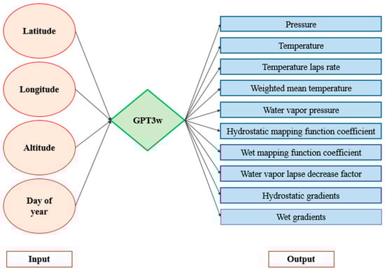
Figure 1.
The input and output parameters for GPT3w model.
The value of the wet refractivity index can be calculated using the water vapor pressure () and temperature () (in Kelvin unit), as follows [9]:
where the values of the , , and coefficients are about , , and , respectively. As stated, by using the monthly average of atmospheric parameter for estimating the mean, annual, and semiannual coefficients of GPT3w, accuracy of the represented wet refractivity indices may be decreased. Therefore, in this study, a branch of the neural network has been used to improve the accuracy of the GPT3w model.
3.2. Radio Occultation Observation
By passing through the Earth’s atmosphere, the refractivity indices cause the GNSS signals to bend off [37]. This bending signal is seen by the LEO satellites that carry GNSS receivers on the other side of the Earth. By implementing the RO technique, this signal can be utilized to retrieve atmospheric parameters. By applying the precise orbit and clock information of both GNSS and LEO satellites, the excess phases compelled by atmosphere effects can be calculated and used to retrieve the bending angle profiles [20]. After that, this bending angle can be inverted to wet refractivity profiles, using the Abel inversion method. Further details about data processing can be found in [37].
RO provides valuable meteorological parameter profiles, such as temperature, pressure, and water vapor pressure, with high accuracy, global coverage, and vertical resolution [20]. In fact, the US-Taiwan mission Constellation Observing System for Meteorology, Ionosphere, and Climate (COSMIC 1/2) [38] provides about 2500 RO events per day and plays a key role in studying the atmosphere [39]. With the advance of space science, more LEO satellites with onboard GNSS receivers have recently been launched, thereby providing a dense dataset for the observation of changes in atmospheric parameters. By employing the measurements of pressure, temperature, and water vapor pressure of these RO observations, the wet refractivity index can be calculated as in [7].
In this study, to construct a dense dataset for training ELM, the RO observations from COSMIC 1/2, Gravity Recovery and Climate Experiment (GRACE) [40], Korea Multi-Purpose Satellite-5 (KOMPSAT-5) [41], Meteorological Operational satellite (MetOP) A/B/C [42], and TerraSAR-X (TSX) [43] have been used. These observations were obtained from https://cdaac-www.cosmic.ucar.edu/cdaac/ (accessed on 1 December 2022). It is worth mentioning that the RO observations of MetOP-A from the year 2007 to 2016 are labeled as MetOP-A-2016, and those of 2016–2022 as MetOP-A. Figure 2 shows the availability of the RO observations covering 2007–2022. In this figure, the RO observations shown by the blue color are applied for training the ELM and those in red are considered for evaluating the performance of ELM.
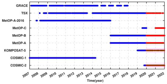
Figure 2.
An overview of the availability of RO observations over Iran, covering 2007–2022. The blue color indicates observations that are used for training the ELM and those in red represent those applied for testing the outputs of ELM.
3.3. Region of Study
The RO observations from various missions are extracted over Iran (~44.5 to 62.5° in longitude and 25.5 to 39.5° in latitude). The study area is located at the mid-latitude zone that exhibits subtropical climate, bringing a variety of atmospheric circulations [37]. In this region, the altitude ranges approximately from −37 to 2426 m and drives many local features in water vapor distribution, alongside different geographical phenomena. To apply the RO observations, the study area is discretized into patches in both the latitude and longitude directions, i.e., 285 patches used for training ELM. The value of the wet refractivity indices is almost zero at altitudes higher than 10 km [4]; thus, in each patch, the observations above 10.5 km are disregarded. Figure 3 shows the discretization of the study area and the number of RO observations used for training and testing.
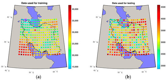
Figure 3.
An overview of the number of RO observations used in resolution patches for (a) training and (b) testing the ELM. The patch with the least RO observations for the training step has been shown with magenta borders around it in (a).
The patch with the least RO observations (14,094 observations) for the training step is shown by the magenta borders in Figure 3 (Longitude 46.5 and Latitude 39.5). The day of the year versus the altitude representation of RO observations for this patch is displayed in Figure 4. According to this figure, the contained observations have an appropriate coverage for both the altitude and the day of the year.
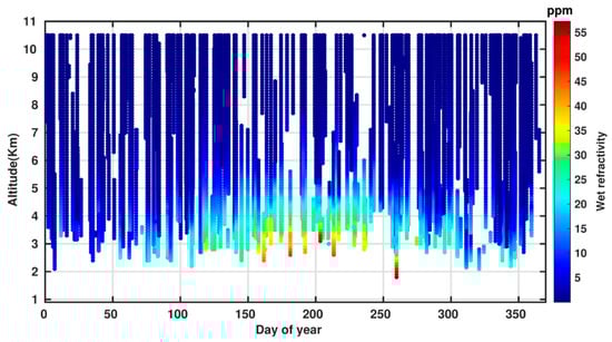
Figure 4.
RO observations of training dataset in the patch (longitude 46.5 and latitude 39.5) with the minimum number of observations.
Radiosonde stations provide observations of the temperature, pressure, dew point temperature, and relative humidity at different altitudes, alongside precipitable water at the station [44]. These observations are provided at 12 and 24 UTC every day. Due to the high accuracy, this type of observation has been widely used for evaluating the modelling results [4,6,23,45]. To evaluate the radiosonde measurements, Survo et al. 2015 [46] compared precipitable water from radiosonde measurements with microwave radiometer observations and GPS, where their results showed an agreement of about 1 mm. Therefore, this validation is considered in this study, too. Using the radiosonde measurements, one can estimate water vapor pressure () as [4]:
where represents the temperature in degree Celsius; is the measured relative humidity; and the constant coefficients , , and are , and respectively [47]. Therefore, by using Equation (7), the value of the wet refractivity index can be calculated. In this study, six radiosonde stations are considered, whose locations can be seen in Figure 5.
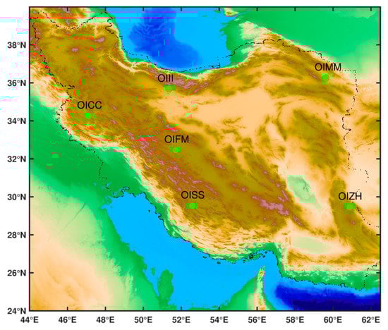
Figure 5.
Locations of the six radiosonde stations used in this study.
For evaluating the results, the RMSE, Correlation Coefficients (), Mean Absolute Error (MAE), and Refined Willmott Index (RWI) statistical values are used, which can be calculated, respectively, as [4,25,48]:
where and represent the estimated and target values, respectively, and is the mean target value. For each considered case, the best performance is identified as the one associated with increasing the CC and RWI values or with decreasing the RMSE and MAE values.
4. Results and Discussion
4.1. Determining the ELM Hyper Parameters
To construct ELM, at first, the variables in the input layer and the number of neurons in the hidden layer must be specified. In fact, these parameters greatly affect the accuracy of the estimated solution. For example, the lack of neurons in the hidden layer may lead to a model that does not capture all the structure of the data. In contrast, too many neurons in the hidden layer might result in over-parameterization and introducing biases to the solution [23]. Therefore, three sets of input parameters are tested in this study that are taken from the GPT3w model, including (1) [Temperature, Water vapor pressure], (2) [Pressure, Temperature, Water vapor pressure], and (3) [Pressure, Temperature, Water vapor pressure, Wet atmospheric gradients], and the range of the number of neurons in the hidden layer are changed from 2 and 40. Afterward, for each considered set of input parameters (1, 2, and 3) and the number of neurons in the hidden layer (2 to 40), ELM is trained using the RO observations of 2007–2020 (for 285 patches separately). By utilizing the trained ELM, the wet refractivity indices for the RO test dataset in each patch have been estimated, and by comparison with the target values, the RMSEs of all contained RO observations are calculated. The set of input layer parameters and the number of hidden layers with the minimum RMSE are then considered the desired ELM setup.
Figure 6 shows the RMSE values for these experiments, where we found that the maximum RMSE values are related to the scenario with two numbers of neurons in the hidden layer for the three considered sets of input parameters. Then, the RMSE value decays, along with increasing the number of neurons, and by reaching to about eight neurons, the slope becomes flat. As indicated in this figure, by considering two parameters in the input layer (Temperature and Water vapor pressure), the solution converges faster to the corresponding minimum RMSE value, compared to the one with five parameters (compare the red curve with the green). We can also observe that a model with 14 neurons in the hidden layer provides the best results in terms of RMSE value. Therefore, ELM has been developed using these hyperparameters (5 sets of input parameters and 14 neurons in the hidden layer). The structure of the implemented ELM is shown in Figure 7. For the chosen ELM, for one arbitrary patch, the weights and biases of the hidden layer, as well as those of the output layer, are provided as a supplementary “ELM_weights.mat” file, along with the corresponding instructor text file.
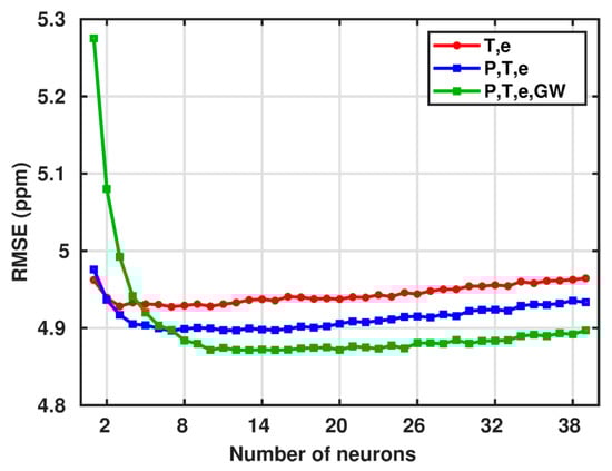
Figure 6.
The RMSE value for different numbers of neurons in the hidden layer of the ELM; the red, blue, and green lines indicate [Temperature and Water vapor pressure], [Pressure, Temperature and Water vapor pressure], and [Pressure, Temperature, Water vapor pressure and Wet atmospheric gradients] as input parameters for the ELM, respectively.
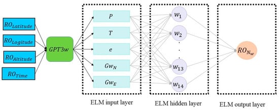
Figure 7.
An overview of the parameters and layers in the ELM. The model is built for 285 patches.
4.2. Comparison with the RO Observation
The constructed ELM models are applied to estimate the wet refractivity indices along the RO observations of 2020–2022. Figure 8a shows the ELM- and GPT3w-derived wet refractivity indices over Iran in comparison with the corresponding RO observations. Further, Figure 8b,c show the Taylor diagrams for the calculated RMSE and correlation coefficient values, as well as the MAE and RWI values for this comparison, respectively.
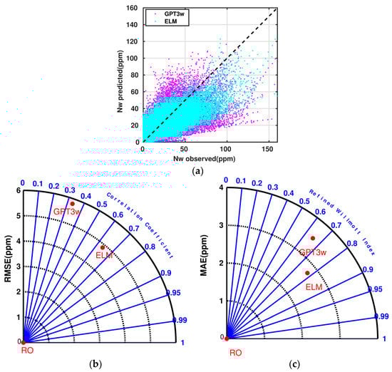
Figure 8.
(a) Comparison of the ELM and GPT3w wet refractivity indices with the RO observations; (b) Calculated RMSE and correlation coefficients for ELM and GPT3w in the Taylor diagram; (c) Calculated MAE and Refined Willmott Index for ELM and GPT3w in the Taylor diagram.
Particularly, Figure 8b indicates that the RMSE value for the ELM estimated wet refractivity indices is about 4.8 ppm, which shows an improvement of about 17%, compared with the corresponding GPT3w model value. Moreover, the correlation coefficient values for ELM are found to be about 0.64, i.e., ~1.9 times greater than that of GPT3w. The MAE and RWI values are shown in Figure 8c. According to this figure, the MAE values for ELM and GPT3w are about 2.7 and 3.5 ppm, respectively, which corresponds to an improvement of about 21% in the MAE value. Furthermore, the ELM RWI value shows an improvement of about 13% in comparison with the corresponding GPT3w value.
To show the performance of ELM over different altitudes, the region of study has been divided into five altitude levels. Afterward, the estimated wet refractivity indices from the test dataset between each altitude level have been compared with the corresponding RO observations. Figure 9 shows the Taylor diagram for the RMSE and correlation coefficients value, alongside the Taylor diagram for the MAR and Refined Willmott Index for ELM and GPT3w at the assessed altitudes. It is noteworthy that the red and blue points correspond to the ELM and GPT3w statistics, respectively.
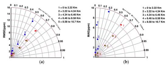
Figure 9.
(a) The comparison of the RMSE and correlation coefficient value for the ELM and GPT3w at different altitudes; (b) The comparison of the MAE and RWI value for the ELM and GPT3w at different altitudes. The red and blue points correspond to ELM and GPT3w statistic parameters, respectively.
According to Figure 9a, the RMSE values of ELM and GPT3w are found to be larger for low-altitude levels due to the fact that most of the water vapor content is concentrated at these altitudes, and the wet refractivity indices at lower altitudes are larger than those at higher altitudes. This fact can also be seen in Figure 9b for the MAE values in the low-altitude levels. It can also be observed that the greatest improvement in the CC values corresponds to the first altitude level, where water vapor content is mostly concentrated, and the corresponding wet refractivity indices show high variability within the spatial and temporal domains. Therefore, it can be inferred from Figure 9 that by implementing ELM using the RO observations, the higher incensement in accuracy is achieved in the most crucial altitudes.
Figure 10 shows the values of RMSE and MAE for the comparison of the ELM and GPT3w wet refractivity indices with the corresponding RO observations over 24 months, from 1st January of the year 2020 to 1st January of the year 2022 (during the validation period).
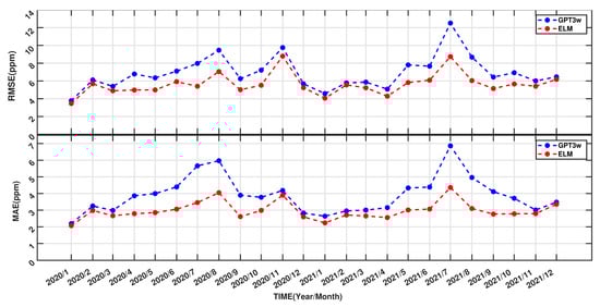
Figure 10.
The monthly RMSE and MAE values for the comparison of the ELM and GPT3w wet refractivity indices with the corresponding RO observations.
We found that the RMSE and MAE values of ELM are lower than those of the corresponding GPT3w (the mean RMSE values for GPT3w and ELM are about 7 and 5.6 ppm, respectively, and also, the mean MAE values for GPT3w and ELM are about 3.9 and 2.9 ppm, respectively) during all considered evaluation periods. The results confirm that this technique can be used for different time periods.
4.3. Comparison with the Radiosonde Observation
For further evaluation, our estimations of wet refractivity indices are compared with six radiosonde stations in the study region (stations are shown in Figure 5). This comparison is done over the period of 1 January 2020–31 December 2020, where data were available to use. The collected measurements of the radiosonde stations data are used to compute the wet refractivity index profiles from the station altitude to 10 Km above the surface of the Earth. Figure 11 shows the comparison of the ELM and GPT3w wet refractivity indices with the corresponding radiosonde stations observations. Additionally, the mean RMSE over 10 different altitudes is depicted in this figure.
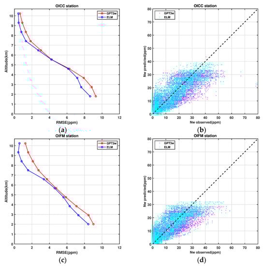
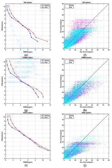
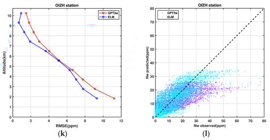
Figure 11.
Comparison of the ELM- and GPT3w-derived wet refractivity indices with the corresponding radiosonde observations at six stations within Iran. The mean RMSE values for 10 different altitude levels are shown. Figures (a,c,e,g,i,k) represent the RMSE at different altitudes, and figures (b,d,f,h,j,l) represent the comparison of the ELM and GPT3w wet refractivity indices with the in-situ radiosonde observations.
Figure 11 indicates that, in each radiosonde station, the mean RMSE values from ELM are lower than those of the corresponding GPT3w model at different altitudes. A summary of the corresponding statistic values for each station is shown in Figure 12.
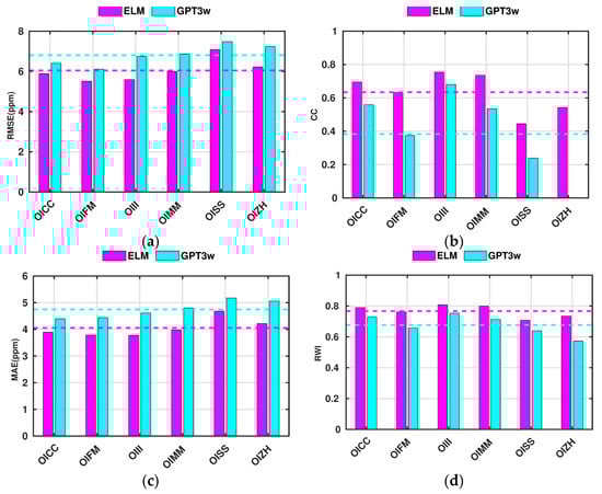
Figure 12.
The RMSE (in subplot (a)), CC (in subplot (b)), MAE (in subplot (c)), and RWI (in subplot (d)) values for the comparison of the ELM and GPT3w wet refractivity indices with the corresponding radiosonde observations at six stations of this study. The cyan and magenta colors represent the mean value of the statistical measures derived from the ELM and GPT3w models, respectively.
Figure 12 indicates that the mean RMSE and MAE values for ELM are about 6 and 4 ppm. These values are found to be about 14% and 14.5% lower than that of the GPT3w model. Moreover, the mean CC value for ELM is about 0.63, which is 1.7 times better than the CC values of GPT3w. In addition, the mean RWI value for ELM is about 0.77, which is 10% higher than the corresponding GPT3w value. From Figure 12, it can be seen that the GPT3w CC value is about −0.1, which shows a negative correlation between radiosonde and GPT3w wet refractivity indices. However, implementing ELM raised the CC value up to 0.54, which indicates the good performance of ELM at this location.
5. Conclusions
Increasing the accuracy of existing models that provide atmospheric parameters will lead to more reliability in weather forecast skills and monitoring of climate change. Water vapor content or wet refractivity indices are substantial atmospheric parameters that exhibit considerable variability in space and time. By using empirical models, the atmospheric parameters can be obtained for desired locations. Among these models, Global Pressure and Temperature 3 (GPT3w) is the latest version of the GPT model series that can provide several atmospheric parameters to be included in weather forecasting skills or for satellite-based positioning purposes. This model is based on the monthly mean data of the ERA-Interim numerical model, with a spatial resolution of about one degree in both the latitude and longitude directions. However, due to the lack of permanent monitoring stations, the accuracy of empirical models is decreased in some regions. With the emerging Radio Occultation (RO) technique, the opportunity has been provided to measure atmospheric parameters in high spatial-temporal resolution, with no geographical limitation.
In this study, the RO observation was used to improve the accuracy of the GPT3-derived wet refractivity indices over Iran, which suffers from a lack of permanent meteorological or GNSS stations. For this purpose, an Extremely Learning Machine (ELM) technique was developed, in which the atmospheric parameters from the GPT3w model were used in the input layer. The corresponding wet refractivity indices from the RO technique were placed as the target parameters in the output layer in order to train the neural network. To train the ELM, the RO observations of 2007–2020 were utilized. Afterward, the estimated wet refractivity indices from ELM were compared with the corresponding RO observations from the year 2020 to the year 2022. The numerical results showed that by considering Pressure, Temperature, Water vapor pressure, and Wet atmospheric gradients as parameters for the ELM input layer, the RMSE and MAE values decreased by about 17 and 21 percent, respectively, compared to the original GPT3w values. Additionally, the correlation coefficient value from ELM was about 0.63, which was about 1.9 times better than that from the corresponding GPT3 model. Moreover, the result shows an improvement of about 13 percent in the ELM RWI values.
For further investigation, the estimated wet refractivity indices from ELM were also compared with the data of six located radiosonde stations covering the year 2020. This comparison resulted in an improvement of about 14 and 14.5 percent in the average RMSE and MAE values of the wet refractivity indices, respectively, as well as a higher correlation coefficient (1.7 times) and RWI values.
Future works may focus on presenting a global model for estimating wet refractivity indices, using artificial neural networks. Additionally, further investigations can be done for combining different sources of atmospheric observation, such as GNSS-estimated ZWD or onboard radiometer observations from altimetry missions, alongside RO observations for improving the estimation of wet refractivity indices using ANN.
Supplementary Materials
The following supporting information can be downloaded at: https://www.mdpi.com/article/10.3390/atmos14010112/s1.
Author Contributions
All authors have contributed equally to preparing this manuscript. All authors have read and agreed to the published version of the manuscript.
Funding
Ehsan Forootan was supported by the Danmarks Frie Forskningsfond [10.46540/2035-00247B], i.e., the DFF2 re-search project DANSk-LSM.
Institutional Review Board Statement
Not applicable.
Informed Consent Statement
Not applicable.
Data Availability Statement
The RO data are freely accessible.
Conflicts of Interest
The authors declare no conflict of interest.
References
- Alshawaf, F.; Balidakis, K.; Dick, G.; Heise, S.; Wickert, J. Estimating trends in atmospheric water vapor and temperature time series over Germany. Atmos. Meas. Tech. 2017, 10, 3117. [Google Scholar] [CrossRef]
- Stierman, E. Precipitable Water Vapour Estimation Using GPS in Uganda: Measuring and Modelling the Precipitable Water Vapour Using Single and Dual Frequency GPS Receivers. Master’s Thesis, Delft University of Technology, Delft, The Netherlands, 2017. [Google Scholar]
- Bevis, M.; Businger, S.; Herring, T.A.; Rocken, C.; Anthes, R.A.; Ware, R.H. GPS meteorology: Remote sensing of atmospheric water vapor using the Global Positioning System. J. Geophys. Res. Atmos. 1992, 97, 15787–15801. [Google Scholar] [CrossRef]
- Forootan, E.; Dehvari, M.; Farzaneh, S.; Khaniani, A.S. A functional modelling approach for reconstructing 3 and 4 dimensional wet refractivity fields in the lower atmosphere using GNSS measurements. Adv. Space Res. 2021, 68, 4024–4038. [Google Scholar] [CrossRef]
- Haji-Aghajany, S.; Amerian, Y.; Verhagen, S.; Rohm, W.; Ma, H. An optimal troposphere tomography technique using the WRF model outputs and topography of the area. Remote Sens. 2020, 12, 1442. [Google Scholar] [CrossRef]
- Adavi, Z.; Mashhadi-Hossainali, M. 4D tomographic reconstruction of the tropospheric wet refractivity using the concept of virtual reference station, case study: Northwest of Iran. Meteorol. Atmos. Phys. 2014, 126, 193–205. [Google Scholar] [CrossRef]
- Böhm, J.; Möller, G.; Schindelegger, M.; Pain, G.; Weber, R. Development of an improved empirical model for slant delays in the troposphere (GPT2w). GPS Solut. 2015, 19, 433–441. [Google Scholar] [CrossRef]
- Penna, N.; Dodson, A.; Chen, W. Assessment of EGNOS tropospheric correction model. J. Navig. 2001, 54, 37–55. [Google Scholar] [CrossRef]
- Liu, Z.; Chen, X.; Liu, Q. Estimating zenith tropospheric delay based on GPT2w model. IEEE Access 2019, 7, 139258–139263. [Google Scholar] [CrossRef]
- Bender, M.; Dick, G.; Ge, M.; Deng, Z.; Wickert, J.; Kahle, H.-G.; Raabe, A.; Tetzlaff, G. Development of a GNSS water vapour tomography system using algebraic reconstruction techniques. Adv. Space Res. 2011, 47, 1704–1720. [Google Scholar] [CrossRef]
- Aghajany, S.H.; Amerian, Y. Three dimensional ray tracing technique for tropospheric water vapor tomography using GPS measurements. J. Atmos. Sol.-Terr. Phys. 2017, 164, 81–88. [Google Scholar] [CrossRef]
- Haji-Aghajany, S.; Amerian, Y.; Verhagen, S. B-spline function-based approach for GPS tropospheric tomography. GPS Solut. 2020, 24, 88. [Google Scholar] [CrossRef]
- Hersbach, H.; Bell, B.; Berrisford, P.; Hirahara, S.; Horányi, A.; Muñoz-Sabater, J.; Nicolas, J.; Peubey, C.; Radu, R.; Schepers, D. The ERA5 global reanalysis. Q. J. R. Meteorol. Soc. 2020, 146, 1999–2049. [Google Scholar] [CrossRef]
- Dee, D.P.; Uppala, S.M.; Simmons, A.J.; Berrisford, P.; Poli, P.; Kobayashi, S.; Andrae, U.; Balmaseda, M.; Balsamo, G.; Bauer, D.P. The ERA-Interim reanalysis: Configuration and performance of the data assimilation system. Q. J. R. Meteorol. Soc. 2011, 137, 553–597. [Google Scholar] [CrossRef]
- Whitaker, J.S.; Hamill, T.M.; Wei, X.; Song, Y.; Toth, Z. Ensemble data assimilation with the NCEP global forecast system. Mon. Weather. Rev. 2008, 136, 463–482. [Google Scholar] [CrossRef]
- Yang, F.; Guo, J.; Zhang, C.; Li, Y.; Li, J. A regional zenith tropospheric delay (ZTD) model based on GPT3 and ANN. Remote Sens. 2021, 13, 838. [Google Scholar] [CrossRef]
- Böhm, J.; Heinkelmann, R.; Schuh, H. Short note: A global model of pressure and temperature for geodetic applications. J. Geod. 2007, 81, 679–683. [Google Scholar] [CrossRef]
- Lagler, K.; Schindelegger, M.; Böhm, J.; Krásná, H.; Nilsson, T. GPT2: Empirical slant delay model for radio space geodetic techniques. Geophys. Res. Lett. 2013, 40, 1069–1073. [Google Scholar] [CrossRef]
- Landskron, D.; Böhm, J. VMF3/GPT3: Refined discrete and empirical troposphere mapping functions. J. Geod. 2018, 92, 349–360. [Google Scholar] [CrossRef]
- Xu, X.; Luo, J.; Shi, C. Comparison of COSMIC radio occultation refractivity profiles with radiosonde measurements. Adv. Atmos. Sci. 2009, 26, 1137–1145. [Google Scholar] [CrossRef]
- Chen, P.; Yao, Y.; Yao, W. Global ionosphere maps based on GNSS, satellite altimetry, radio occultation and DORIS. GPS Solut. 2017, 21, 639–650. [Google Scholar] [CrossRef]
- Al-Fanek, O.J.S. Ionospheric Imaging for Canadian Polar Regions. Ph.D. Thesis, University of Calgary, Calgary, AB, Canada, 2013. [Google Scholar]
- Xia, P.; Cai, C.; Liu, Z. GNSS troposphere tomography based on two-step reconstructions using GPS observations and COSMIC profiles. Ann. Geophys. 2013, 31, 1805–1815. [Google Scholar] [CrossRef]
- Dettmering, D.; Schmidt, M.; Heinkelmann, R.; Seitz, M. Combination of different space-geodetic observations for regional ionosphere modeling. J. Geod. 2011, 85, 989–998. [Google Scholar] [CrossRef]
- Forootan, E.; Farzaneh, S.; Lück, C.; Vielberg, K. Estimating and predicting corrections for empirical thermospheric models. Geophys. J. Int. 2019, 218, 479–493. [Google Scholar] [CrossRef]
- Ji, E.Y.; Moon, Y.J.; Park, E. Improvement of IRI global TEC maps by deep learning based on conditional Generative Adversarial Networks. Space Weather 2020, 18, e2019SW002411. [Google Scholar] [CrossRef]
- Weng, L.; Lei, J.; Zhong, J.; Dou, X.; Fang, H. A machine-learning approach to derive long-term trends of thermospheric density. Geophys. Res. Lett. 2020, 47, e2020GL087140. [Google Scholar] [CrossRef]
- Suparta, W.; Alhasa, K.M. Modeling of Tropospheric Delays Using ANFIS; Springer: Berlin/Heidelberg, Germany, 2016. [Google Scholar]
- Pal, M. Extreme-learning-machine-based land cover classification. Int. J. Remote Sens. 2009, 30, 3835–3841. [Google Scholar] [CrossRef]
- Huang, G.-B.; Zhu, Q.-Y.; Siew, C.-K. Extreme learning machine: Theory and applications. Neurocomputing 2006, 70, 489–501. [Google Scholar] [CrossRef]
- Kardani, N.; Bardhan, A.; Samui, P.; Nazem, M.; Zhou, A.; Armaghani, D.J. A novel technique based on the improved firefly algorithm coupled with extreme learning machine (ELM-IFF) for predicting the thermal conductivity of soil. Eng. Comput. 2022, 38, 3321–3340. [Google Scholar] [CrossRef]
- Bardhan, A.; Samui, P.; Ghosh, K.; Gandomi, A.H.; Bhattacharyya, S. ELM-based adaptive neuro swarm intelligence techniques for predicting the California bearing ratio of soils in soaked conditions. Appl. Soft Comput. 2021, 110, 107595. [Google Scholar] [CrossRef]
- Raja, M.N.A.; Shukla, S.K. An extreme learning machine model for geosynthetic-reinforced sandy soil foundations. Proc. Inst. Civ. Eng.-Geotech. Eng. 2022, 175, 383–403. [Google Scholar] [CrossRef]
- Zhao, T.; Pan, S.; Gao, W.; Qing, Z.; Yang, X.; Wang, J. Extreme learning machine-based spherical harmonic for fast ionospheric delay modeling. J. Atmos. Sol.-Terr. Phys. 2021, 216, 105590. [Google Scholar] [CrossRef]
- Le, X.-H.; Ho, H.V.; Lee, G.; Jung, S. Application of long short-term memory (LSTM) neural network for flood forecasting. Water 2019, 11, 1387. [Google Scholar] [CrossRef]
- Ben-Israel, A.; Greville, T.N. Generalized Inverses: Theory and Applications; Springer Science & Business Media: Berlin/Heidelberg, Germany, 2003; Volume 15. [Google Scholar]
- Sharifi, M.A.; Sam-Khaniani, A.; Joghataei, M.; Schmidt, T.; Masoumi, S.; Wickert, J. Tropopause analysis over the Iranian region using GPS radio occultation data. Adv. Space Res. 2013, 52, 1700–1707. [Google Scholar] [CrossRef]
- Rocken, C.; Ying-Hwa, K.; Schreiner, W.S.; Hunt, D.; Sokolovskiy, S.; McCormick, C. COSMIC system description. Terr. Atmos. Ocean. Sci. 2000, 11, 21–52. [Google Scholar] [CrossRef]
- Anthes, R.; Sjoberg, J.; Feng, X.; Syndergaard, S. Comparison of COSMIC and COSMIC-2 Radio Occultation Refractivity and Bending Angle Uncertainties in August 2006 and 2021. Atmosphere 2022, 13, 790. [Google Scholar] [CrossRef]
- Tapley, B.D.; Bettadpur, S.; Watkins, M.; Reigber, C. The gravity recovery and climate experiment: Mission overview and early results. Geophys. Res. Lett. 2004, 31. [Google Scholar] [CrossRef]
- Cho, S.; Chung, J.; Park, J.; Yoon, J.; Chun, Y.; Lee, S. Radio Occultation Mission in Korea Multi-Purpose Satellite KOMPSAT-5. In New Horizons in Occultation Research; Springer: Berlin/Heidelberg, Germany, 2009; pp. 275–283. [Google Scholar]
- Klaes, D.; Holmlund, K. The EPS/Metop system: Overview and first results. In Proceedings of the Joint 2007 EUMETSAT Meteorological Satellite Conference and the 15th Satellite Meteorology & Oceanography Conference of the American Meteorological Society, Amsterdam, The Netherlands, 24–28 September 2007; pp. 24–28. [Google Scholar]
- Werninghaus, R.; Buckreuss, S. The TerraSAR-X mission and system design. IEEE Trans. Geosci. Remote Sens. 2009, 48, 606–614. [Google Scholar] [CrossRef]
- Durre, I.; Vose, R.S.; Wuertz, D.B. Overview of the integrated global radiosonde archive. J. Clim. 2006, 19, 53–68. [Google Scholar] [CrossRef]
- Bender, M.; Raabe, A. Preconditions to ground based GPS water vapour tomography. Ann. Geophys. 2007, 25, 1727–1734. [Google Scholar] [CrossRef]
- Survo, P.; Leblanc, T.; Kivi, R.; Jauhiainen, H.; Lehtinen, R. Comparison of selected in-situ and remote sensing technologies for atmospheric humidity measurement. In Proceedings of the 19th Conference on Integrated Observing and Assimilation Systems for the Atmosphere, Ocean and Land Surface, Phoenix, AZ, USA, 4–8 January 2015. [Google Scholar]
- International Telecommunication Union. Recommendation ITU-R P.453-9, The Radio REFRACTIVE index: Its Formula and Refractivity Data; Recommendations and Reports of the ITU-R; International Telecommunication Union: Geneva, Switzerland, 2001; Volume 8, pp. 617–618. [Google Scholar]
- Raja, M.N.A.; Shukla, S.K. Predicting the settlement of geosynthetic-reinforced soil foundations using evolutionary artificial intelligence technique. Geotext. Geomembr. 2021, 49, 1280–1293. [Google Scholar] [CrossRef]


Disclaimer/Publisher’s Note: The statements, opinions and data contained in all publications are solely those of the individual author(s) and contributor(s) and not of MDPI and/or the editor(s). MDPI and/or the editor(s) disclaim responsibility for any injury to people or property resulting from any ideas, methods, instructions or products referred to in the content. |
© 2023 by the authors. Licensee MDPI, Basel, Switzerland. This article is an open access article distributed under the terms and conditions of the Creative Commons Attribution (CC BY) license (https://creativecommons.org/licenses/by/4.0/).