Abstract
Climate model evaluation work has made progress both in theory and practice, providing strong support for better understanding and predicting climate change. However, at the weather scale, there is relatively little assessment of climate models in terms of daily-scale climate phenomena, such as storm frequency and intensity. These weather-scale variables are of significant importance for our understanding of the impacts of climate change. In order to assess the capability of climate models to simulate weather-scale climate patterns, this study employs Self-Organizing Maps (SOMs) for weather pattern classification. By combining different evaluation metrics, varying the number of SOM types, changing the size of the study area, and altering the reference datasets, the climate models are evaluated to ensure the robustness of the assessment results. The results demonstrate that the size of the study area is positively correlated with observed differences, and there are correlations among different evaluation metrics. The highest correlation is observed between evaluation metrics in large-scale and small-scale spatial domains, while the correlation with SOM size is relatively low. This suggests that the choice of evaluation metrics has a minor impact on model ranking. Furthermore, when comparing the correlation coefficients calculated using the same evaluation metrics for different-sized regions, a significant positive correlation is observed. This indicates that variations in the size of the study area do not significantly affect model ranking. Further investigation of the relationship between model performance and different SOM sizes shows a significant positive correlation. The impact of dataset selection on model ranking is also compared, revealing high consistency. This enhances the reliability of model ranking. Taking into account the influence of evaluation metric selection, SOM size, and reanalysis data selection on model performance assessment, significant variations in model ranking are observed. Based on cumulative ranking, the top five models identified are ACCESS1-0, GISS-E2-R, GFDL-CM3, MIROC4h, and GFDL-ESM2M. In conclusion, factors such as evaluation metric selection, study area size, and SOM size should be considered when assessing model ranking. Weather pattern classification plays a crucial role in climate model evaluation, as it helps us better understand model performance in different weather systems, assess their ability to simulate extreme weather events, and improve the design and evaluation methods of model ensemble predictions. These findings are of great significance for optimizing and strengthening climate model evaluation methods and provide valuable insights for future research.
1. Introduction
Global Climate Models (GCMs) are important tools in studying climate change [1]. The climate model is an important approach for studying climate change and formulating adaptation strategies [2]. Given the diverse and complex natural environment in China, it is necessary to adjust model parameters and evaluate simulation results based on the characteristics of the region when conducting climate model capability assessment [3]. This ensures accurate simulation results that align with the specific characteristics of the regional climate system in China [4]. The assessment of climate model capability not only facilitates a deeper understanding of the evolution of the regional climate system, but also enhances prediction accuracy and reliability, providing a solid foundation for developing effective strategies to address climate change [5]. However, due to the complexity of the global climate system, GCMs have limitations in their representativeness and reliability, particularly in simulating extreme precipitation events [6]. The ability of models to simulate extreme precipitation is directly linked to the accuracy of future projections. Furthermore, atmospheric circulation is considered a key driver of extreme precipitation [7,8], making it a focus in model evaluations.
The current assessment of climate models has made significant progress in both theory and practice, providing strong support for a better understanding and prediction of climate change [9]. Firstly, in recent years, the ensemble approach using multiple models has been widely applied in climate model evaluation. Studies have shown that averaging the output results of multiple models can reduce the errors caused by individual model biases, thereby improving the accuracy and reliability of simulation results. This ensemble method has been successfully applied in global-scale climate simulations, but still faces challenges in simulating weather-scale phenomena [10]. Secondly, the application of statistical metrics enables objective assessment of model performance. Commonly used metrics, such as mean error, root-mean-square error, correlation, and variance, are widely used to evaluate the differences between model outputs and observational data. These metrics provide a quantitative way to compare the discrepancies between model output and actual observations, helping us judge the accuracy and reliability of the models [11]. However, there are still some issues in the current climate model evaluation. Particularly, at the weather scale, there is relatively limited evaluation of climate phenomena at the daily scale, such as storm frequency and intensity. These weather-scale variables are of vital importance in our understanding of the impacts of climate change [12].
Weather regime classification is an important method for evaluating and diagnosing the performance of global climate model output [13]. With the rapid development of computer technology, an increasing number of meteorologists have adopted weather regime classification techniques to categorize and analyze various weather systems globally, such as low-pressure systems, cyclones, and vortices [14]. These classification techniques can be used to discover the physical factors and processes associated with specific weather patterns and, based on that, further comprehend the mechanisms behind global climate change [15]. For instance, Pfahl et al. proposed a spatial clustering-based approach to classify weather regimes with similar atmospheric circulation features from reanalysis data, aiming to unveil the relationship between global climate change and extreme weather events [16]. Other studies have employed weather regime classification techniques by integrating multiple weather indices for multivariate regression analysis, effectively reducing biases and errors in meteorological model output [17]. Additionally, machine learning algorithms have also been utilized to classify global climate models, offering better handling of nonlinear and high-dimensional data compared to traditional physics-based structures [18]. In summary, weather regime classification techniques serve as essential tools for assessing the reliability and diagnosing the performance of meteorological models, uncovering underlying physical rules within weather systems, and providing crucial support for research on global climate change [19].
Classification techniques of weather patterns have been applied to assess GCM outputs and evaluate model performance, as well as diagnose changes in atmospheric circulation [20,21]. In recent years, self-organizing maps (SOMs) have emerged as a useful tool for assessing the skill of climate models in capturing climate patterns and variability. The use of self-organizing maps (SOMs) and discretized Sammon maps to study the links between atmospheric circulation and weather extremes was explored by Stryhal and Plavcová [22]. The complex relationships between atmospheric circulation and weather extremes were investigated, contributing to a better understanding of these connections. Climate extremes were studied using SOMs by Gibson et al. [23], while precipitation patterns were analyzed using SOMs by Li et al. [24]. These studies showcased the potential of SOMs in examining climate-related phenomena. The performance of CMIP5 models in simulating synoptic patterns over East Asia was evaluated by Wang et al. [25], and synoptic systems in CMIP5 models over the Australian region were assessed by Gibson et al. [26]. These investigations aimed to improve climate modeling by assessing the accuracy of model simulations. SOMs were employed by Gore et al. [27] to establish connections between large-scale meteorological patterns and extratropical cyclones in CMIP6 climate models. This study demonstrated the capability of SOMs in linking meteorological patterns to cyclones. Future changes in tropical cyclogenesis were investigated using SOMs by Jaye et al. [28], contributing to an enhanced understanding of the potential unfolding of these changes. Event-specific drought attribution was explored by Harrington et al. [29] using SOMs, providing insights into the potential of SOMs in attributing drought events to specific causes. The performance of CMIP5 and CMIP6 models in simulating the East Asian summer monsoon was compared by Yu et al. [30], while boreal summer circulation patterns of CMIP6 models over the Asian region were evaluated by Bu et al. [31]. These studies aimed to evaluate and improve the ability of climate models to simulate regional climate phenomena. The reviewed studies demonstrate the effectiveness of self-organizing maps as a tool for climate model evaluation. They offer comprehensive assessments of climate model performance, reveal model strengths and weaknesses, and provide valuable insights into their ability to capture climate patterns and variability.
The Pacific Subtropical High (PTH) and its interaction with Tropical Low Pressure (TLP) play a crucial role in shaping the summer weather conditions of East Asia. Previous studies have found that the interannual variability of the western ridge of the PTH is closely associated with the region’s summer rainfall [32]. Specifically, when the western ridge shifts southward, it leads to a reduction in rainfall across East Asia. In a comprehensive review, researchers summarized previous research on the relationship between the PTH and summer precipitation in East Asia. They highlighted the significant influence of tropical low-pressure systems in modulating this relationship. These systems contribute to the complex pressure distribution pattern observed during the summer season, impacting the spatial distribution and intensity of rainfall [33]. Studies focusing on the variability of the western PTH and its connection with the East Asian summer monsoon have demonstrated that anomalous changes in the high-pressure system have important implications for the monsoon, consequently influencing the climate and weather patterns of East Asia [34]. Moreover, investigations into the Pacific–East Asian teleconnection, with an emphasis on the influence of El Niño–Southern Oscillation (ENSO) events on the East Asian climate, have established a close linkage between El Niño events and the Pacific–East Asian Teleconnection, which further affects the climate dynamics of the region, including the behavior of the PTH [35]. In summary, the PTH and its interaction with tropical low-pressure systems significantly influence the summer weather conditions in East Asia. The position of the PTH’s western ridge is closely associated with changes in rainfall patterns. The interplay between the PTH and tropical low-pressure systems contributes to the complex pressure distribution pattern observed during the summer, impacting rainfall intensity and distribution. Additionally, the variability of the PTH exerts important influences on the East Asian summer monsoon, and the influence of ENSO events on the Pacific–East Asian Teleconnection further shapes regional climate dynamics. Based on the analysis and summary presented above, we can identify several limitations in previous research: (a) There is a lack of comprehensive evaluation considering multiple variables. Previous research tends to focus on evaluating individual variables, and the ranking of models may differ for different variables. (b) The causes of extreme precipitation are complex. There is not a one-to-one correspondence between extreme precipitation and weather patterns, making it challenging to analyze the relationship between extreme precipitation and atmospheric circulation. (c) Model rankings may vary with different regions.
We aim to select models that can effectively simulate extreme precipitation and atmospheric circulation. Firstly, we aim to extend the single-variable evaluations of GCMs to a comprehensive evaluation considering multiple variables. Secondly, a new model evaluation approach is needed to investigate whether models can realistically reproduce the patterns of atmospheric circulation and the corresponding extreme precipitation. Thirdly, we are particularly interested in the applicability of the new method to China and identifying models that perform well in China. To address these issues, we apply the proposed new method to select GCMs that perform best in China. This analysis will provide insights into why these models perform well and can serve as a reference for model improvement. Additionally, it can guide future climate predictions and downscaling of model selection.
This study aims to achieve two primary objectives. Firstly, it proposes a novel approach for evaluating models using weather pattern classification, which assesses whether precipitation patterns are generated accurately. Secondly, we apply this new model evaluation approach to Southeastern China. The approach is used to comprehensively assess the ability of GCMs in simulating atmospheric circulation patterns, and to select a set of high-performing GCMs.
2. Data
2.1. Analysis Domains
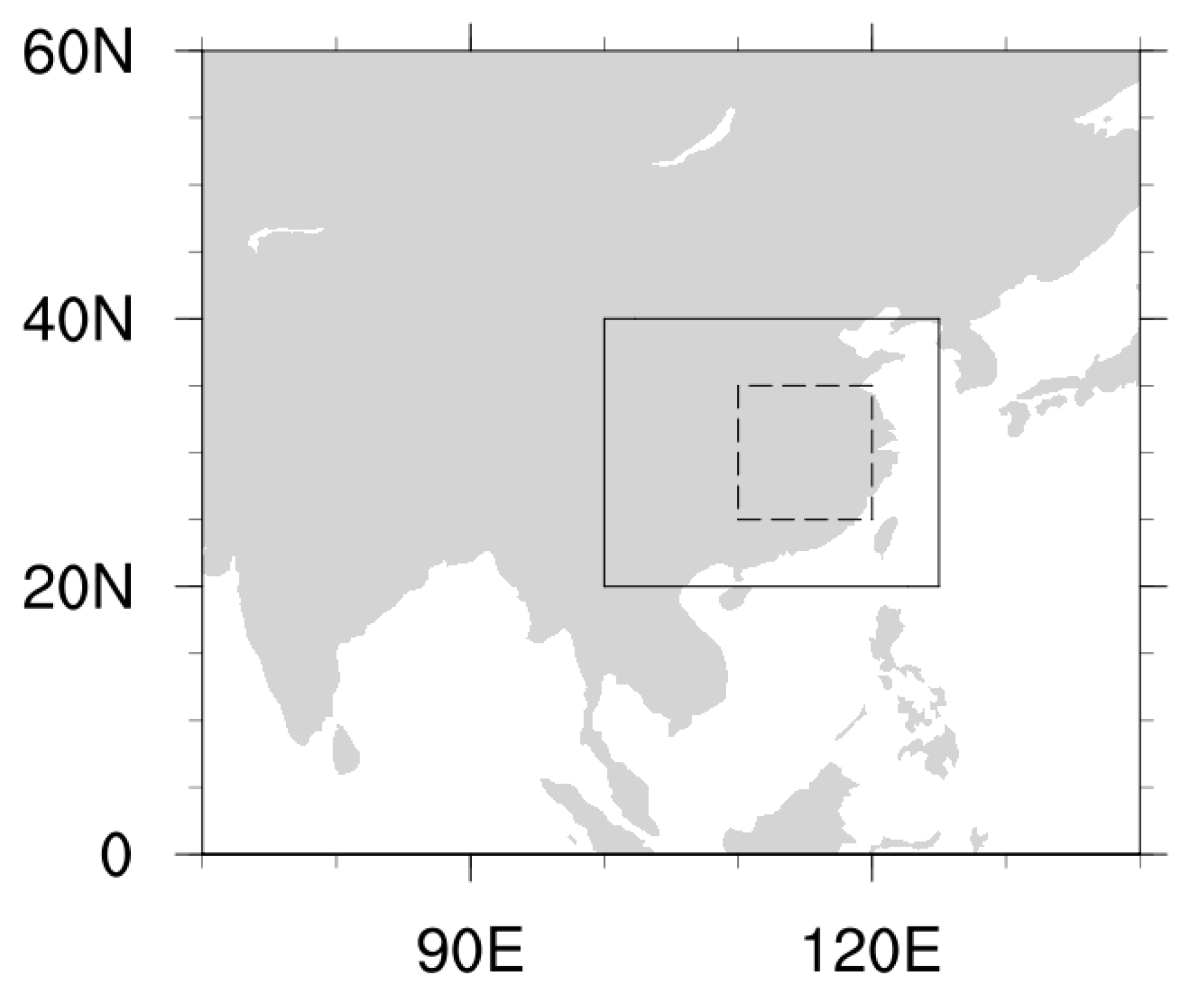
To explore the sensitivity of the analysis results to changes in the study area, we conducted the analysis on three spatial domains: (a) the “large” domain, encompassing the majority of central and eastern China; (b) the “small” domain, covering Southeastern China (Figure 1). The latitude range of a larger region is between 20° N and 40° N, while the longitude range is between 100° E and 125° E. The latitude range of a smaller region is between 25° N and 35° N, while the longitude range is between 110° E and 120° E. This region covers a vast geographical area in China, including diverse terrains and climate conditions. In terms of climatology, it encompasses various climate zones and precipitation patterns in China, ranging from subtropical humid climate to temperate continental climate, as well as highland climate and arid climate [36]. This study area also includes significant geographical features of China, such as the Yangtze River Basin, the Yellow River Basin, and the Qinghai–Tibet Plateau. Conducting climatological research in this region contributes to a deeper understanding of China’s climate change trends, precipitation patterns, and their impacts on ecosystems, agriculture, and urban planning. This is of great significance for tackling climate change, resource management, and sustainable development [37,38].

Figure 1.
Analytical regions: The “large/broad” region (larger rectangle) encompasses the majority of central and eastern China. The latitude range of the area is 20° N to 40° N, and the longitude range is 100° E to 125° E. The “ small/narrow” region (rectangle within the broad one) is situated in Southeastern China. The latitude range of the area is 25° N to 35° N, and the longitude range is 110° E to 120° E. This approach aims to examine potential variations in the analytical outcomes resulting from modifications in the scope of the study area.
2.2. Validation Data
To evaluate the ability of Global Climate Models (GCMs) to accurately simulate weather patterns and their impact on precipitation, the study compares the historical simulations of GCMs with reference datasets, including reanalysis data and observation data. Two variables, namely, mean sea level pressure (MSLP) and precipitation (PR), are used for the evaluation.
As the reference dataset, MSLP is derived from reanalysis data, which are widely considered to be the most reliable dataset [39]. Two sets of reanalysis data are utilized in this study: the National Center for Environmental Prediction/National Center for Atmospheric Research (NCEP-NCAR) [40] dataset and the 40-year European Centre for Medium-Range Weather Forecasts (ECMWF) Re-Analysis (ERA-40) [41] dataset. These reanalysis datasets are chosen as they are regarded as the most reliable datasets for comparison with GCM output data [39].
Both reanalysis datasets provide MSLP data with a regular resolution of 2.5° × 2.5°. For the analysis, a 20-year period (1980–1999) from each reanalysis dataset is selected as the reference period for this study. Despite its relatively short duration, this 20-year period includes the most complete and accurate observational data, largely due to advancements in space-based remote sensing [42].
In addition to the reanalysis data, gridded precipitation (PR) data provided by Chen et al. [43] are also used (referred to as CHEN05). This dataset has a spatial resolution of 0.5° × 0.5° and is obtained by ordinary kriging interpolation from 753 operational surface stations of the China Meteorological Administration. The dataset exhibits minimal interpolation errors in the eastern part of China due to the high station density.
By comparing the GCMs’ simulations with these reference datasets, the study aims to assess the accuracy of the models in reproducing weather patterns, specifically MSLP and precipitation. The use of reliable reanalysis data and observation data, along with the high-quality gridded precipitation data, enhances the robustness of the evaluation. This approach provides valuable insights into the performance of GCMs and their ability to simulate real-world weather conditions.
2.3. Model Output
To ensure that the Self-Organizing Map (SOM) method accurately captures daily weather-scale precipitation events, this study utilized daily sea level pressure (SLP) and precipitation (PR) data from 34 Coupled Model Intercomparison Project Phase 5 (CMIP5) models [44]. The data were obtained from the Program for Climate Model Diagnosis & Intercomparison (PCMDI) archive website (https://esgf-node.llnl.gov/projects/cmip5: accessed on 3 September 2022). A time frame of 20 years, specifically from 1980 to 1999, was selected for analysis.
Each CMIP5 model has its own unique resolution, which is provided in Table 1. To facilitate comparison and analysis, all models were interpolated to a common grid with a resolution of 2.5° × 2.5°.

Table 1.
Model identification, originating center, and atmospheric resolution. The symbol ‘~’ represents ‘approximately equal to’.
By utilizing the SLP and PR data from these CMIP5 models, the study aims to accurately capture and analyze daily precipitation events at a weather scale. The chosen time frame allows for a comprehensive assessment of the models’ performance over a significant period. The interpolation of the models’ data onto a common grid enables consistent and meaningful comparisons among the different models.
This approach ensures the capture of valuable information regarding daily precipitation patterns, enabling a thorough investigation of the models’ ability to simulate weather-scale events. The inclusion of multiple models from the CMIP5 dataset enhances the robustness and reliability of the analysis.
3. Methods
3.1. Classification of WT: Self-Organizing Maps (SOMs)
The Self-Organizing Map (SOM) is an unsupervised artificial neural network that utilizes competitive learning to identify similarities in nonlinear phases of synoptic-scale circulation. It represents the weather system as distinct neuron clusters through self-learning and iterative comparison, enabling the modeling and classification of atmospheric circulation.
The SOM consists of an input layer and a competitive (output) layer, with training and mapping being the two main steps. In this study, daily mean sea level pressure fields are used as the input layer for the SOM. Specific types of circulation patterns, called nodes, are identified by the competitive layer, with the number of nodes being user-defined.
The general algorithm for SOM training involves the following steps: First, the SOM network is established and initialized using SOM nodes (or reference vectors) to represent the input data. Each node is initialized with a weight vector. In each iteration, each reference vector gradually learns from the input data by updating its weight. This is achieved by calculating the Euclidean distance between the weight vector of each node and the input vector. The node with the smallest Euclidean distance to the input vector is identified as the winning node. The position of nodes within the neighborhood of the winning node is then updated, moving them closer to the input vector and allowing each node to learn and adjust its position based on the input data. This process continues for all input data, resulting in the topological organization of the SOM, where similar nodes are placed adjacent to each other.
During training, the learning rate and neighborhood size are adjusted for each input vector while recalculating the Euclidean distance, determining the winning node, and updating the weights of nodes. The training continues until a preset number of iterations is reached. At the end of the training, the winning nodes represent the distinctive circulation patterns extracted by the SOM.
In this study, we use daily sea level pressure fields as the input layer for the self-organizing map. The SOM identifies specific types of circulation patterns as winning nodes in the output layer, with each category referred to as a node. The number of nodes is determined by the user.
The general algorithm for SOM training can be summarized as follows:
(a) Construct and initialize the SOM network: the SOM starts with a user-defined map size, and the nodes (reference vectors) are initialized to represent the input data, with each node assigned a random weight vector.
(b) Calculate Euclidean distance: compute the Euclidean distance between the weight vector of each node’s reference vector and the input vector. This determines the minimum Euclidean distance between the jth node’s weight vector and the input data.
(c) Determine the winning node: select the node in the competitive layer with the minimum Euclidean distance to the input vector as the winning node.
(d) Update the node’s weight: update the position of nodes near the winning node, moving them closer to the input vector, so that each node can learn from the input data and adjust its position accordingly. The weight vector update can be described using the following equation:
In this formula, t represents the current iteration count, W denotes the weight vector, V represents the input vector. Θ is the constraint function, typically referred to as the neighborhood function, that measures the distance from the best matching unit. α is a time-dependent learning restraint. Repeat this process until all input data are processed, and the SOM organizes based on the minimum Euclidean distance, placing similar nodes adjacent to each other.
(e) Update the learning rate and neighborhood size: adjust the learning rate and neighborhood size for the next input vector and repeat steps (b)–(e).
(f) Determine the stopping condition: the training process continues until it reaches the predefined number of iterations. The final winning node represents the feature pattern extracted by the SOM.
For more detailed information on SOM, please refer to the relevant literature, such as Kohonen [45].
The selection of the Self-Organizing Map (SOM) node size is determined based on the number of major synoptic patterns observed. Mathematically, the size of SOM nodes is determined by maximizing similarity within clusters and minimizing similarity between clusters. In this study, we explore different SOM sizes, specifically 3 × 3, 4 × 4, 5 × 5, and 6 × 6 nodes, to compare the training results. By using multiple SOM sizes, we aim to assess the sensitivity of the model evaluation to the SOM size. A detailed discussion and analysis regarding this aspect can be found in Section 4.3.
The SOMs are trained on a seasonal basis, focusing on the summer months of June, July, and August (JJA). To prepare the input data for SOM training, the daily-averaged mean sea level pressure (MSLP) during the 20-year baseline period (1980–1999) is subtracted from the daily MSLP values at each grid point from both the reanalysis dataset and the output of each GCM. The resulting fields, referred to as temporal MSLP, represent the temporal anomalies of MSLP. A similar procedure is applied to extreme precipitation events, where the daily-averaged precipitation is treated as temporal precipitation (PR).
This study investigates the effect of self-organizing map (SOM) size on pattern recognition and general circulation model (GCM) performance evaluation, based on previous research findings. The results indicate that, after fixing the SOM map size, the sensitivity of pattern recognition in SOM training to the selection of optimization parameters is relatively low. However, for GCM performance evaluation, the choice of SOM size may have a certain impact. In order to accurately capture the details of characteristic sea level pressure (SLP) patterns in each season while maintaining interpretability, this study tries different SOM sizes and ultimately selects four sizes: 3 × 3, 4 × 4, 5 × 5, and 6 × 6. By adopting multiple SOM sizes, it is possible to test the sensitivity of model evaluation to SOM size. The present research adheres to academic writing conventions and aims to offer a scholarly insight into the topic.
3.2. Definition of Extreme Precipitation Patterns (EPPs)
Following the methodology of Zhao et al. [46], we establish a definition for extreme precipitation patterns (EPPs) as follows:
(a) Initially, an abnormal precipitation day is identified at each grid point by comparing the daily precipitation anomaly with the long-term daily climatology. If the deviation exceeds +2.0σ (sigma), which represents the standard deviation of the daily average precipitation for the corresponding calendar day, that day is classified as an abnormal precipitation day. This classification is applied to all grid points within the study domain on a daily basis.
(b) To determine the regional impact of extreme precipitation events, we additionally require that the number of grid cells exceeding the precipitation threshold on any given day exceeds 5% of the total number of grid points within the study domain. Only those days that satisfy this criterion are regarded as extreme precipitation events.
(c) The daily grid-normalized precipitation anomaly is then labeled as an extreme precipitation event. This labeling facilitates the utilization of clustering analysis to identify the corresponding extreme precipitation modes (EPPs).
By defining extreme precipitation patterns in this manner, we can effectively analyze and categorize the occurrence of extreme precipitation events within the study region. This approach aligns with established research practices and enables comparability and consistency in subsequent analyses and discussions.
3.3. Model Evaluation
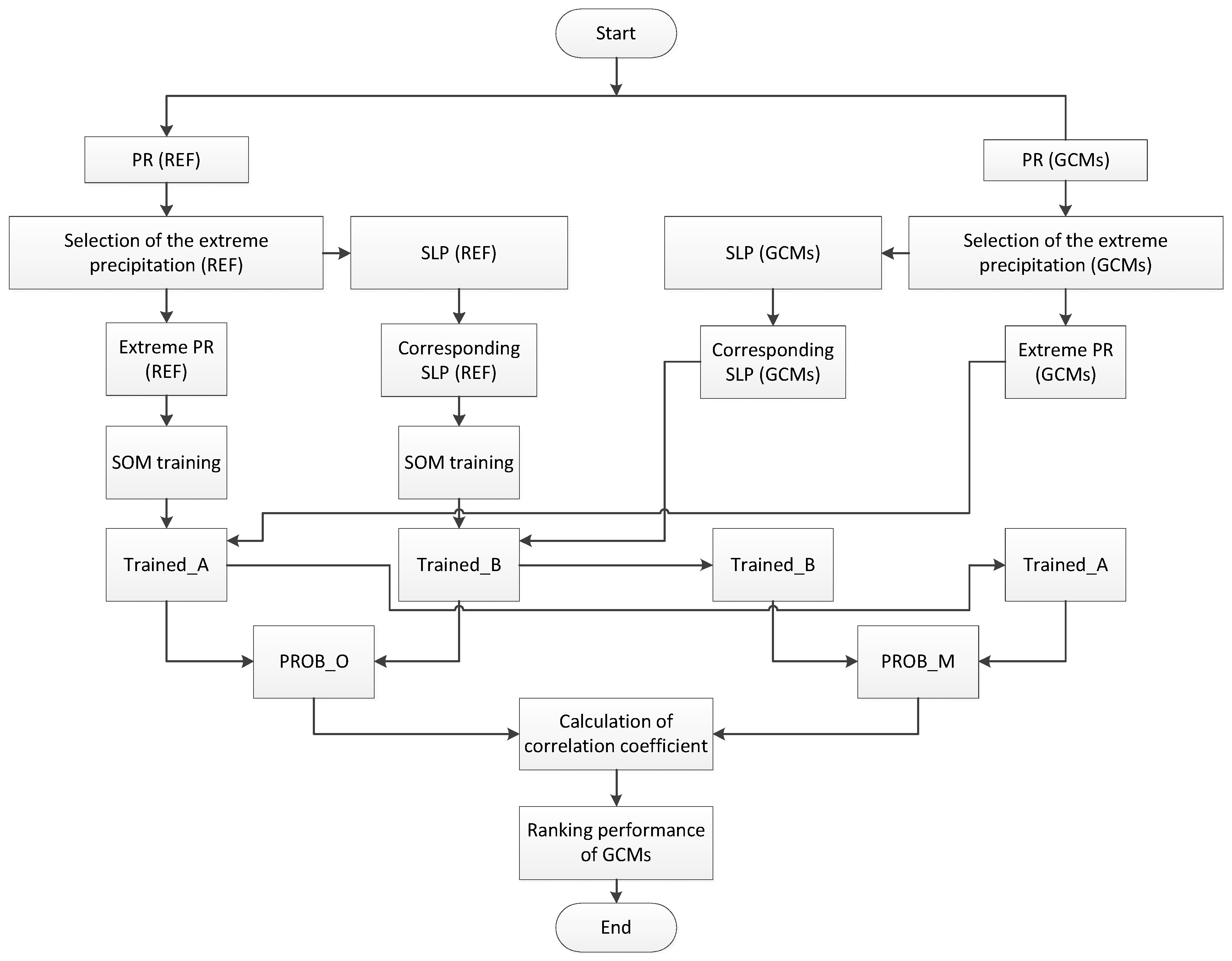
To evaluate the models, we followed the procedure outlined in Section 3.4 to identify days characterized by extreme precipitation events. Precipitation (PR) and mean sea level pressure (MSLP) data corresponding to these identified days were extracted, resulting in two separate datasets. These datasets were then used to train two Self-Organizing Maps (SOMs): Trained_A with MSLP time offset and Trained_B with PR time offset (Figure 2). This training process yielded two distinct models.
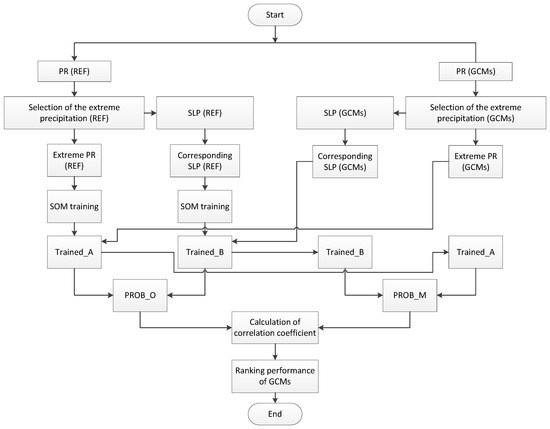
Figure 2.
Methodology: This figure presents the process flowchart illustrating the model evaluation procedure and highlights the key milestones achieved throughout the process.
Subsequently, we conducted an analysis to determine the frequency of occurrence of each element in Trained_A within each element of Trained_B. This frequency analysis enabled the construction of a two-dimensional binary matrix called PROB_O, where each element represents the probability of a specific circulation pattern being associated with extreme precipitation events.
A similar processing method was applied to the model data, resulting in the generation of Trained_A and Trained_B. We then analyzed the frequency of occurrence of each element in Trained_A within each element of Trained_B, yielding a two-dimensional matrix denoted as PROB_M.
To assess the performance of the models, we calculated the correlation coefficient between the reference data (PROB_O matrix) and the model data (PROB_M matrix). The correlation coefficient serves as an indicator of how well the model’s output replicates the observed reanalysis data. A higher correlation coefficient suggests a stronger resemblance between the model’s simulation of extreme precipitation patterns and the reanalysis data.
By evaluating the correlation coefficient, we can determine the accuracy of the models in reproducing extreme precipitation patterns under the same circulation patterns observed in the reanalysis data. This evaluation process ensures the reliability and effectiveness of the models in capturing and representing extreme precipitation events.
3.4. Model Simulation Performance Ranking Metrics
In this paper, we utilized three evaluation metrics, the first two of which were proposed by Radic’ [47], while the last was put forward by Schuenemann and Cassano [48].
- (a)
- Average correlation coefficient
The average correlation coefficients of all seasons (only JJA is considered in this study) and all circulation patterns (3 × 3, 4 × 4, 5 × 5, 6 × 6) were synthesized.
where m is the product of the season number, and four SOM size (m = 4) r is the correlation coefficient. Higher numbers would indicate improved performance.
- (b)
- Cumulative sum of the number of significant correlations
To account for the total number of significant positive correlations, we define a significance measure following the approach in
where is the threshold value for the correlation significantly larger than zero at the 95% confidence level (derived from a t test). The greater the value is, the more favorable the outcome.
- (c)
- Comprehensive rating index
This index can be expressed as
where m is the product of the number of seasons and the size type; n is the number of patterns; and rank is the rating number: the best model has a rank of 1, and the worst is 34. The higher the value is, the better.
In order to obtain the final comprehensive ranking, we can calculate the values of the above three evaluation indexes respectively by analyzing the calculation results of the time anomaly of large and small regions in 20 years (1980–1999).
4. Results
4.1. Simulation of MSLP Temporal Patterns and PR Temporal Patterns
4.1.1. Characteristic Patterns of Mean Sea Level Pressure (MSLP)
The Pacific Subtropical High (PTH) and Tropical Low Pressure (TLP) are significant weather systems that impact summer weather conditions in China. This study investigates the characteristics of these two systems using anomaly pressure distribution charts. The PTH is typically observed as a prominent high-pressure system, exhibiting elevated atmospheric pressures across a broad region. Its presence is associated with prolonged periods of high temperatures, aridity, and reduced rainfall in the southeastern parts of China. The anomaly pressure distribution chart illustrates higher pressure values within this region. In contrast, the TLP is manifested as a weaker low-pressure system, occupying a relatively smaller spatial extent. This system is liable to induce heavy rainfall, storms, and subsequent natural disasters, such as floods and landslides. The anomaly pressure distribution chart depicts lower pressure values within the affected area. When both the PTH and TLP coexist, their distinctive characteristics contribute to a complex pressure distribution pattern on the anomaly pressure distribution chart, resulting in highly variable weather conditions in the southeastern region. Overall, the PTH and TLP are critical components of China’s summer meteorological situation, exerting significant influences on the weather and climate patterns of the southeastern regions.
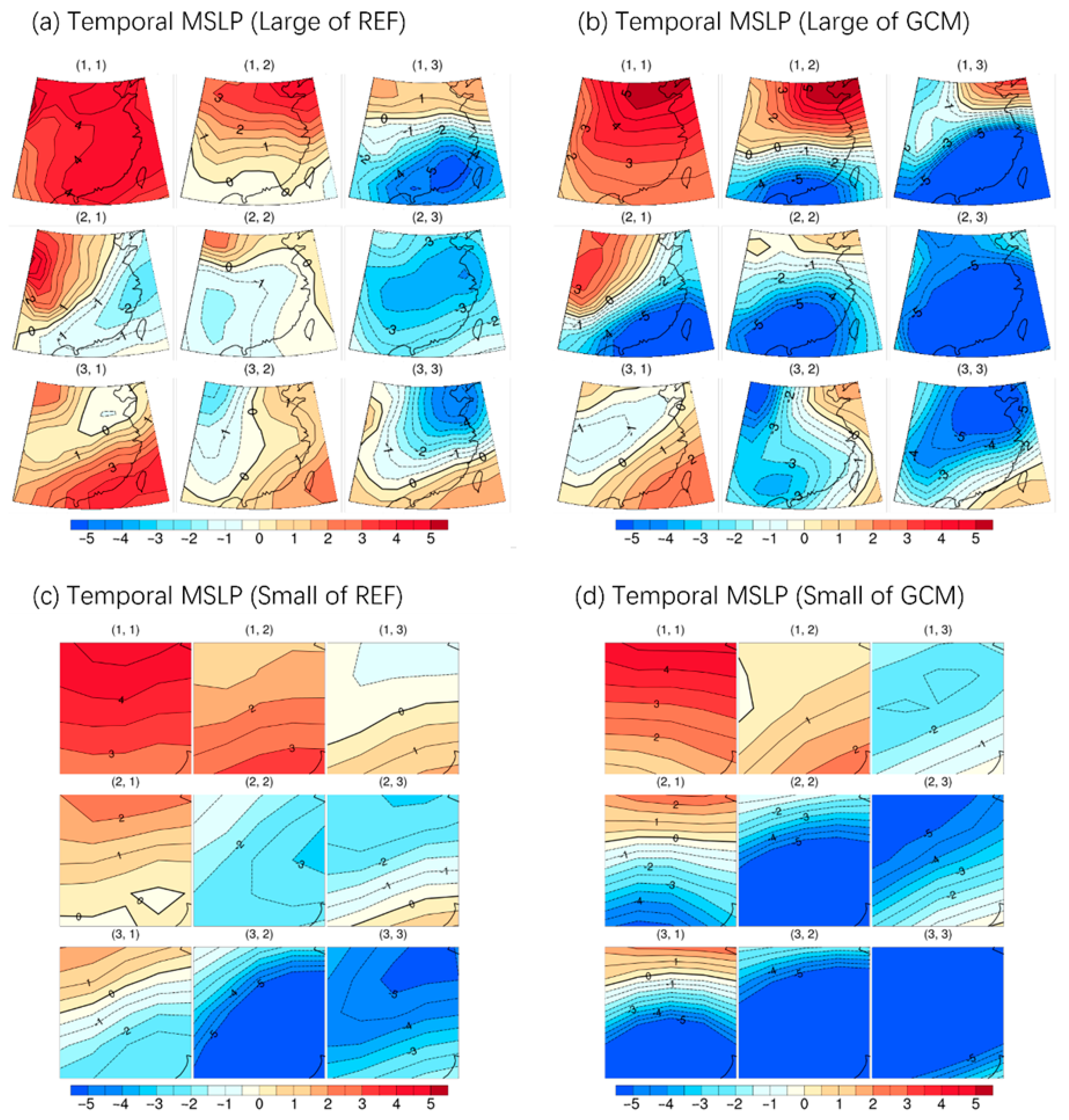
Figure 3a–d depict the characteristic daily patterns of MSLP anomalies during the summer season (June, July, August—JJA) for the period 1980–1999, analyzed using the 3 × 3 Self-Organizing Map (SOM) technique. In this study, we employed the NCEP/NCAR reanalysis dataset (REF) as the reference, along with simulation data from the bcc-csm1-1-m global climate model (GCM).
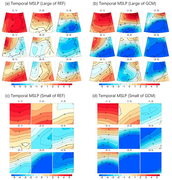
Figure 3.
The 3 × 3 self-organizing maps (SOMs) were employed to analyze the temporal anomalies of mean sea level pressure (MSLP) during the summer season (June, July, and August—JJA). The SOMs were trained using both the reference dataset (REF: NCEP/NCAR reanalysis) and the simulated data from the bcc-csm1-1-m global climate model (GCM) over the baseline period of 1980-1999. Patterns over the large domain (a) of REF and (b) of GCM. Patterns over the small domain (c) of REF and (d) of GCM.
Figure 3a illustrates the spatial distribution of MSLP anomalies over a large area in the REF dataset. Through observation, distinct spatial patterns and variations in MSLP anomalies at a broad scale can be identified. Notably, certain regions exhibit high-pressure or low-pressure systems, which may be associated with local climatic systems and topographical features. These findings align with existing climatological knowledge and offer insights for further investigating the climate mechanisms specific to these regions [32,33,34,35].
Figure 3b presents the corresponding MSLP anomaly patterns from the GCM simulation. By comparing them with the REF dataset, we can evaluate the accuracy and reliability of the GCM in simulating MSLP variability. A strong resemblance between the two indicates a higher reliability of the GCM in reproducing observed climatic phenomena. However, significant discrepancies would necessitate further research to improve and refine the GCM.
Furthermore, Figure 3c showcases the MSLP anomaly patterns within a smaller domain in the REF dataset. Focusing on a more localized analysis enables a detailed examination of pressure variations in specific regions. This localized analysis facilitates a better understanding of the operational mechanisms of small-scale meteorological systems and provides more precise climate predictions and weather forecasts.
Lastly, Figure 3d demonstrates the MSLP anomaly patterns within a smaller domain from the GCM simulation. Comparing the results between the REF dataset and the GCM simulation allows for an assessment of the GCM’s capability to simulate pressure changes at different scales. If the GCM adequately simulates pressure anomalies in local regions, its global-scale simulation results would also gain credibility. However, significant deviations or errors would require further research to enhance the GCM through improved methods and techniques.
In summary, the utilization of the SOM technique allows for a comprehensive analysis of MSLP anomalies during the summer season, enabling the exploration of pressure variations from different scales and perspectives. This analysis enhances our understanding of the intricate nature of the climate system and provides valuable insights for enhancing climate models and prediction capabilities. To gain a more comprehensive understanding of MSLP anomalies, future research can expand the dataset and time range. Additionally, integrating the analysis of other meteorological variables, such as temperature and precipitation, would provide a holistic overview of climate change. This scientific foundation serves as a basis for addressing climate change and mitigating weather-related disasters.
4.1.2. PR Characteristic Patterns
The analysis of precipitation (PR) anomalies during the summer season using the 3 × 3 self-organizing map (SOM) technique offers valuable insights into the spatiotemporal patterns of precipitation. Figure 4a–d illustrate the characteristic daily PR anomaly patterns for the summer season (JJA) over two domains during the period 1980–1999.
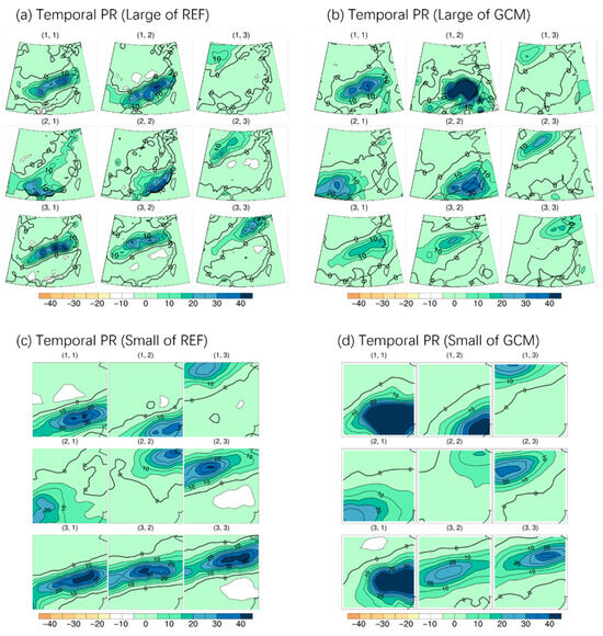
Figure 4.
The temporal anomalies of precipitation (PR) during summer (June, July, August—JJA) were analyzed using 3 × 3 Self-Organizing Maps (SOMs). The SOMs were trained using observations from the reference dataset (REF: CHEN05) and simulations from the bcc-csm1-1-m global climate model (GCM) over the baseline period of 1980-1999. Patterns over the large domain (a) of REF and (b) of GCM. Patterns over the small domain (c) of REF and (d) of GCM.
Figure 4a displays the patterns of PR anomalies over a broad spatial domain in the REF dataset. The SOM analysis reveals distinct spatial structures, indicating the influence of local climate systems and geographical features on precipitation variability during summer. Regions with high PR anomalies may indicate enhanced rainfall, while low PR anomalies can imply drier conditions. These findings align with existing climatological knowledge and highlight the underlying mechanisms driving these patterns.
Figure 4b shows the corresponding patterns of PR anomalies from the GCM simulation, allowing for an assessment of the GCM’s performance in capturing precipitation variability. Consistency and similarity between the two datasets indicate the reliability of the GCM in representing observed PR anomalies. Significant discrepancies between the two datasets emphasize areas for model improvement and refinement, underscoring the importance of continuous model evaluation and development to enhance the accuracy and reliability of climate simulations.
Using the SOM method to classify weather patterns enables a more thorough examination of various precipitation patterns, especially within the smaller spatial range depicted in Figure 4c of the REF dataset. By conducting detailed investigations within these specific regions, we can gain deeper insights into precipitation anomalies and develop an understanding of the operational mechanisms of small-scale meteorological systems that influence these anomalies. This information is of significant importance for improving the accuracy of climate predictions and weather forecasts in these particular areas, as it facilitates a better comprehension and prediction of the development and evolutionary trends of different weather patterns.
Lastly, Figure 4d illustrates the patterns of PR anomalies within a smaller domain from the GCM simulation, enabling the evaluation of the GCM’s ability to capture PR changes at different scales. Comparing the results between the REF dataset and the GCM simulation allows for the assessment of the GCM’s performance in representing PR anomalies in local regions, leading to improved simulations and predictions on a global scale.
The integration of PR anomalies with other meteorological variables, such as temperature and wind patterns, would provide a more comprehensive understanding of climate change and its impacts on regional climate systems. The comparison between the REF dataset and the GCM simulation emphasizes the importance of model evaluation and improvement, highlighting the need for ongoing research efforts to enhance the GCM’s ability to capture precipitation dynamics at multiple spatial scales.
In summary, the SOM technique offers insights into the characteristics and patterns of precipitation variations during the summer season, revealing the influence of local climate systems and geographical features on PR anomalies. These findings align with existing climatological knowledge and provide crucial evidence for understanding the underlying mechanisms driving precipitation dynamics. The localized analysis within smaller spatial domains facilitates a more detailed examination of precipitation patterns in specific regions, improving climate predictions and weather forecasts at local scales. The comparison between the REF dataset and the GCM simulation underscores the importance of ongoing research efforts to enhance the accuracy and reliability of climate simulations and predictions.
4.2. Simulation of Probability
Previous evaluations of the model have primarily focused on assessing its univariate simulation capabilities, and there is limited understanding of the relationship between circulation patterns and precipitation types. To gain a new perspective on the model’s simulation capabilities, we aimed to combine the generation of extreme precipitation with different weather patterns. This involved clustering extreme precipitation events and circulation patterns separately, resulting in an equal number of types for each.
We then calculated the frequency of occurrence for each extreme precipitation type within each weather pattern. This analysis was performed independently for each extreme precipitation type, resulting in matrices as the outcome. The same calculations were executed for each General Circulation Model (GCM), and the results were also organized into respective matrices.
To evaluate the model’s simulation capability, we correlated the matrices derived from each GCM with the corresponding matrix derived from the reanalysis data. A significant positive correlation would indicate that the model effectively simulates the probability of occurrence for each extreme precipitation type within each circulation pattern.
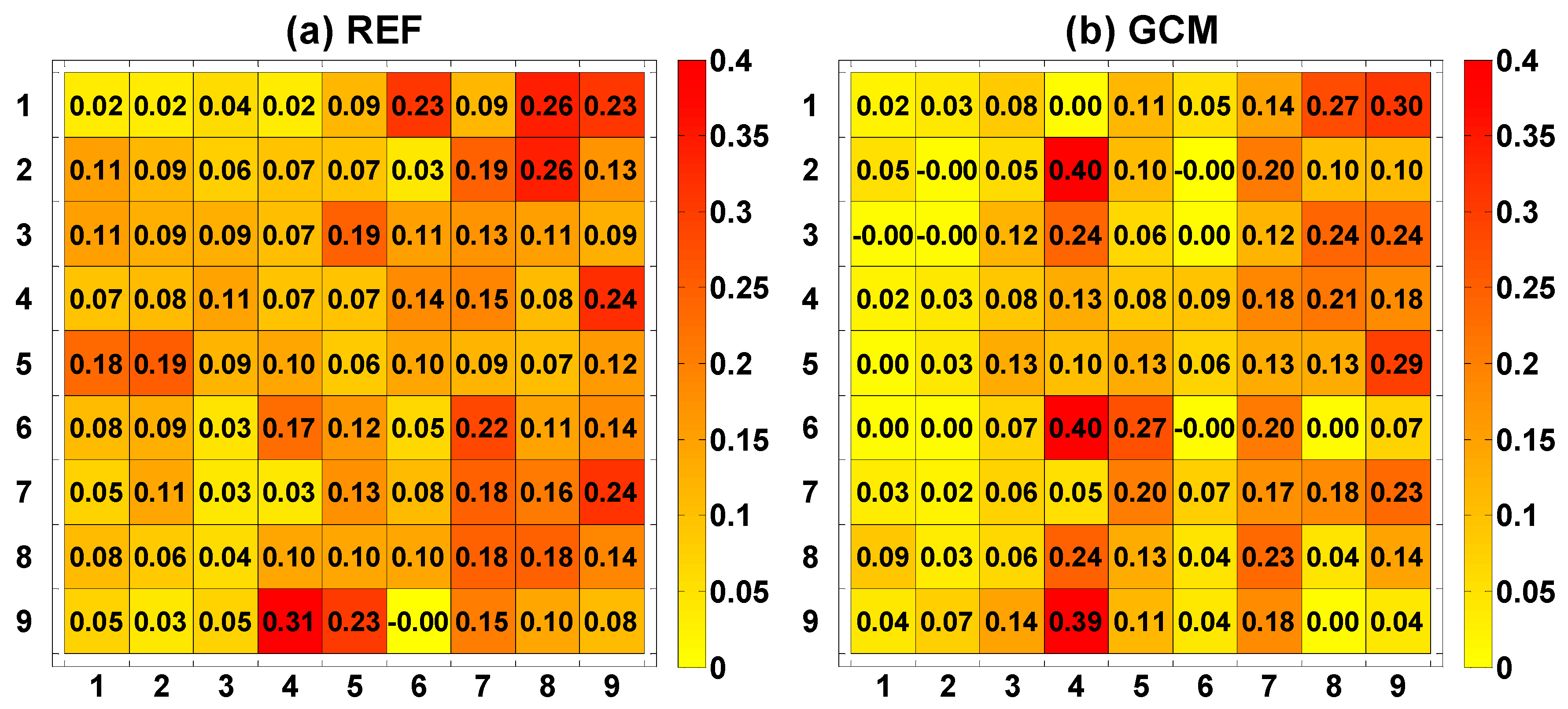
In this study, we established the link between circulation patterns and precipitation types through the use of occurrence probabilities. We will present the analysis results using the bcc-csm1-1-m model as an example. Initially, we calculated the frequency of occurrence for each circulation type within each precipitation type using the reference data (Figure 5). The results showed an uneven distribution, with higher overall frequencies observed on the right side and lower frequencies on the left side of the distribution. The maximum frequency value was found in the last row’s fourth column at the bottom, indicating the potential for different circulation types to yield varying precipitation amounts.
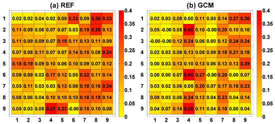
Figure 5.
Comparison of the model’s ability to simulate the probability distribution of occurrence of circulation type in precipitation type (a) of REF (CHEN05 observation) and (b) of GCM (bcc-csm1-1-m).
Subsequently, we performed similar calculations for each model separately. The results for the bcc-csm1-1-m model exhibited a similar uneven distribution pattern as observed in the reference data, with higher frequencies on the right side and lower frequencies on the left side. The maximum frequency values were also concentrated in the fourth column at the bottom, aligning with the reference data. These findings indicate the model’s capability to simulate the correspondence between circulation types and extreme precipitation types.
To quantify the similarity between the frequency distribution matrices, we computed the correlation coefficient. We consider the magnitude of this coefficient as a reliable indicator of the model’s simulation capability, with a higher correlation coefficient indicating superior performance in simulation.
We conducted a correlation analysis between the reference dataset and each General Circulation Model (GCM). We considered different Self-Organizing Map (SOM) sizes (3 × 3, 4 × 4, 5 × 5, 6 × 6) and spatial domains. Table 2 presents the resulting correlation coefficients (r values) for temporal SOMs over the large domain across all SOM sizes. Correlations that were found to be significantly different from zero (at a 95% confidence level) are indicated in bold font. The table shows a wide range of correlation values, which vary across different GCMs and SOM sizes, encompassing both strong positive and negative correlations.
Table 2.
Correlation coefficients (r) between the probability matrices from the observed data and each Global Climate Model (GCM), based on different sizes of Self-Organizing Maps (SOMs) (3 × 3, 4 × 4, 5 × 5, and 6 × 6). The correlations are calculated for both the large domain and the small domain using temporal anomalies of sea level pressure (SLP). Correlation coefficients that are significantly greater than zero at the 95% confidence level are shown in bold font.
Upon analyzing the correlation coefficients, we observed that the majority of the models performed exceptionally well. Out of the 34 GCMs analyzed, 25 exhibited significant positive correlations with the reanalysis data across all SOM sizes. Only three models displayed non-significant correlations at different SOM sizes. The substantial number of significantly positive correlations indicates that nearly every GCM effectively reproduces extreme precipitation patterns as observed in the reanalysis data under the same circulation patterns during the baseline period from 1980 to 1999.
4.3. Model Ranking
4.3.1. Impact of the Choice of Evaluation Indicators on the Assessment of Model Simulation Capacity
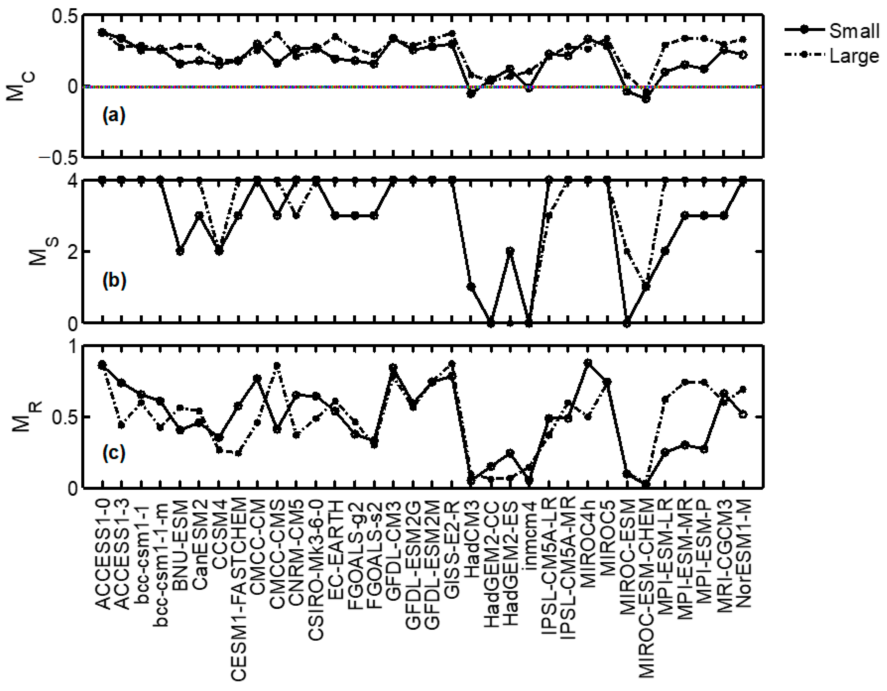
In order to rank GCMs based on their ability to simulate extreme precipitation types, we used a set of evaluation metrics outlined in Section 3.4. Figure 6 depicts the evaluation measures applied to both small and large spatial domains for temporal Sea Level Pressure (SLP) anomaly patterns. Our analysis revealed that the choice of evaluation indicators significantly impacts the assessment results, even when simulating the same climate characteristics.
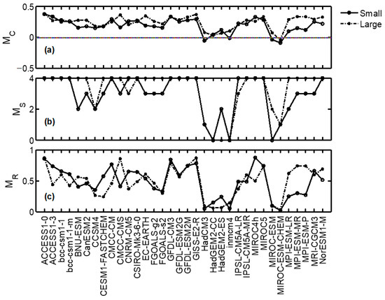
Figure 6.
(top to bottom) (a) Correlation measure , (b) significance measure , and (c) rank measure for each model. The measures are derived for two different cases: SOMs of temporal SLP anomalies over the small domain, and SOMs of temporal SLP anomalies over the large domain.
Figure 6a shows that the evaluation results for model simulation capacity are influenced by the size of the study area. This relationship was also observed for the other two evaluation metrics (Figure 6b,c). However, we found significant correlations between two of the three evaluation indicators, both for the large and small spatial domains, at a 95% confidence level. The correlation coefficients between two indicators, and , were the highest for both domains (0.96 for the large domain and 0.97 for the small domain), while the correlation coefficients between and were the lowest for both domains (0.79 for the large domain and 0.86 for the small domain). These results suggest that although the choice of evaluation metrics has an impact, it has little effect on model ranking.
Our analysis also revealed significant positive correlations between the correlation coefficient calculations for different-sized regions when using the same evaluation metrics. Specifically, the correlation coefficients for the three indicators were 0.74 (), 0.79 (), and 0.63 () between the two spatial domains. Therefore, we conclude that the rankings of patterns are not significantly affected by the size of the study area.
4.3.2. Impact of the Choice of SOM Sizes on the Assessment of Model Simulation Capability
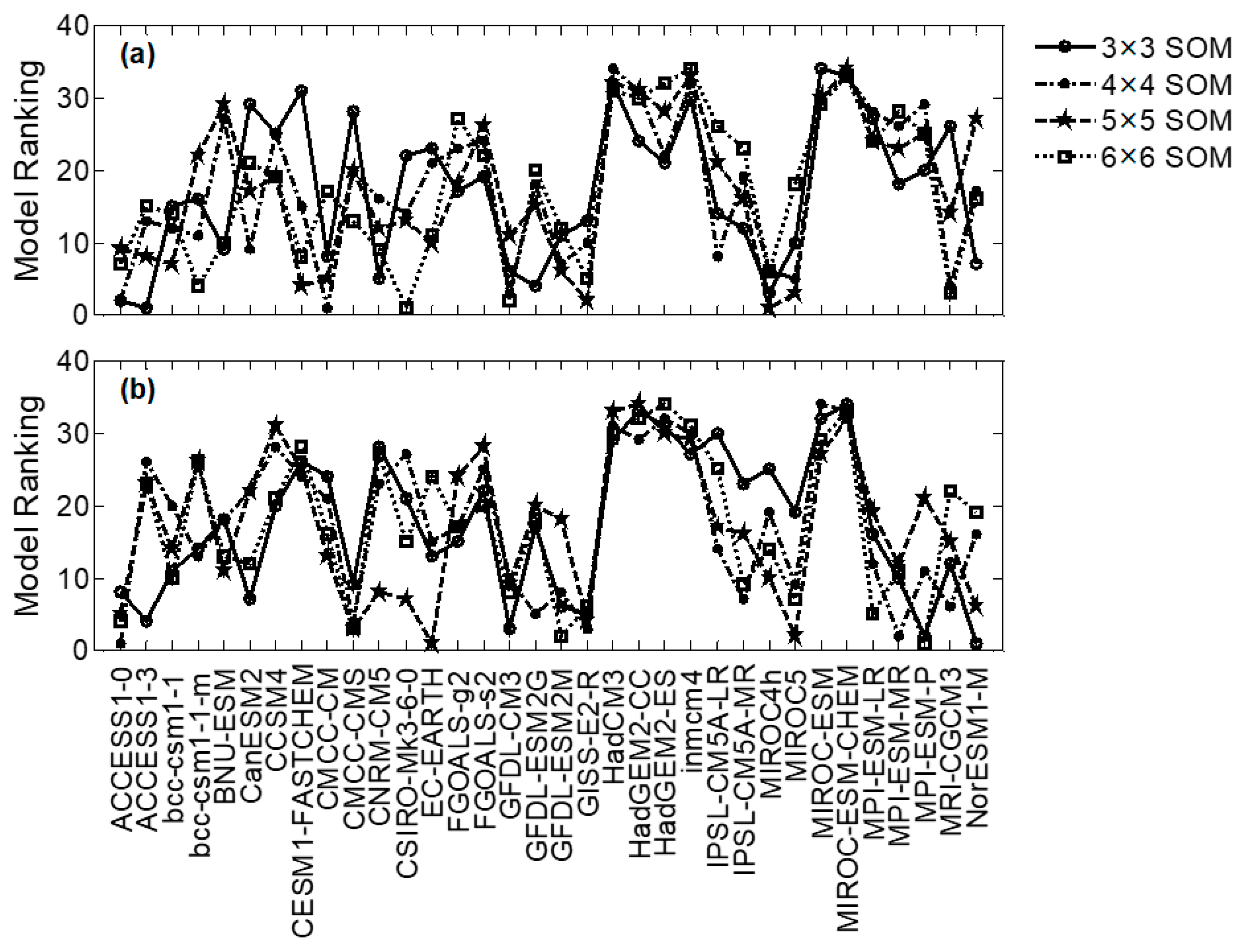
In order to assess the impact of Self-Organizing Map (SOM) sizes on model ranking, we conducted an analysis. Figure 7 presents the results of ranking pairs of models using four different SOM sizes: 3 × 3, 4 × 4, 5 × 5, and 6 × 6. Additionally, we investigated whether there is a relationship between model performances across different SOM sizes, as this would indicate redundancy in evaluation.
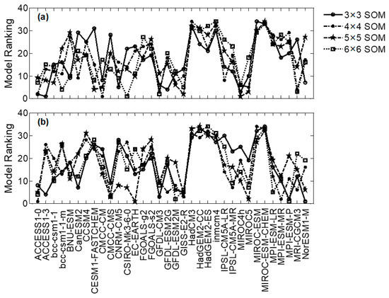
Figure 7.
Model ranking according to the correlation coefficient (R) assessed for four different SOM sizes, 3 × 3, 4 × 4, 5 × 5, and 6 × 6: (a) small domain and (b) large domain.
By correlating the model rankings between two different SOM sizes, we found a significant positive correlation (at a 95% confidence level) for all pairs in both spatial domains. The mean correlation coefficients were calculated to be 0.63 in the small domain and 0.64 in the large domain. These findings suggest that there is consistency in the ranking of models across different SOM sizes, indicating that the choice of SOM size has limited impact on the assessment of model simulation capability.
4.3.3. Impact of the Choice of Reanalysis Data on the Assessment of Model Simulation Capability
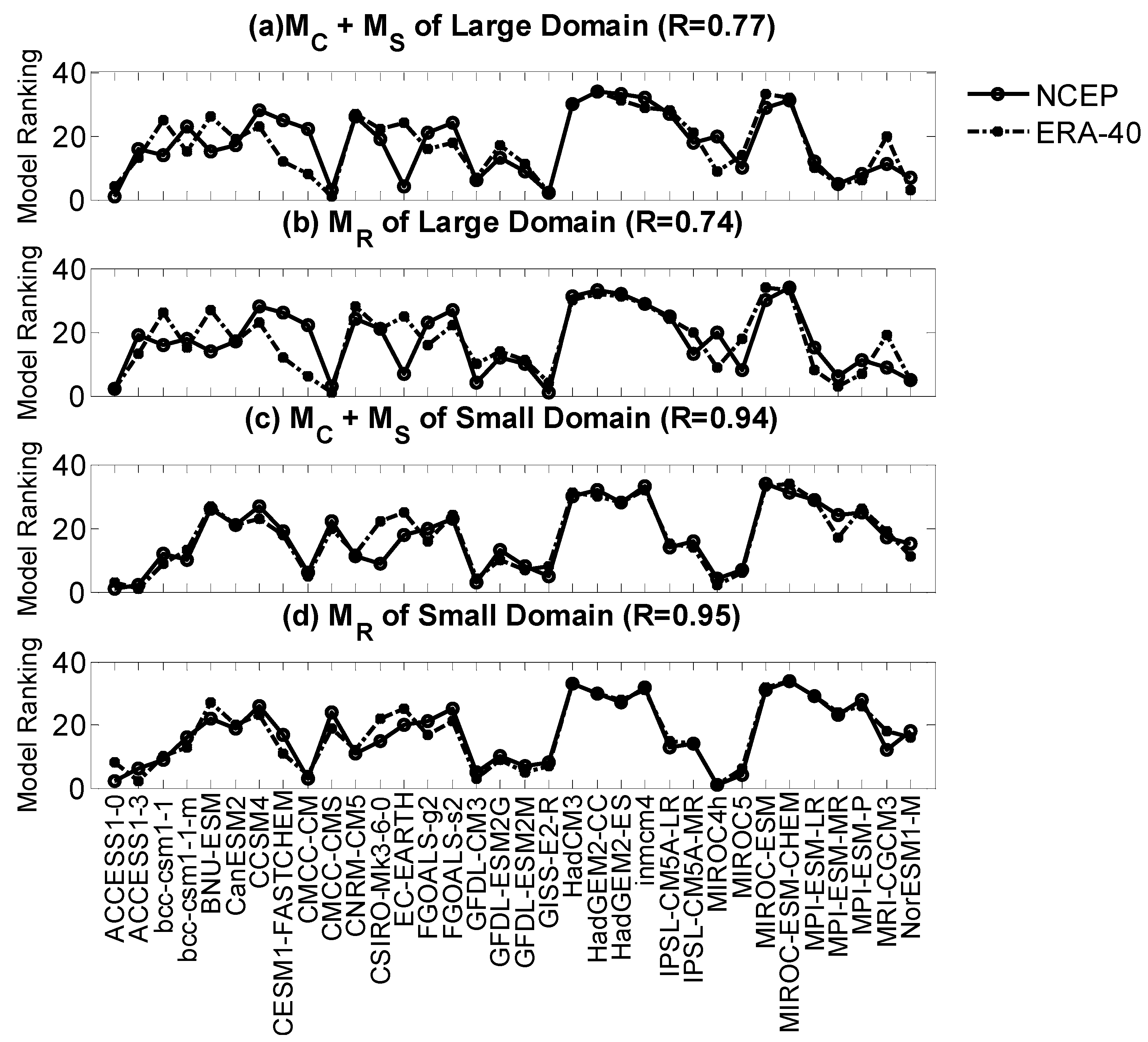
To assess the impact of the choice of reanalysis data on model simulation capability, we separately utilized two different sets of reanalysis data: NCEP and ERA-40. The model ranking results obtained using these datasets are presented in Figure 8. Interestingly, we found a high level of consistency in the model rankings across the two datasets.
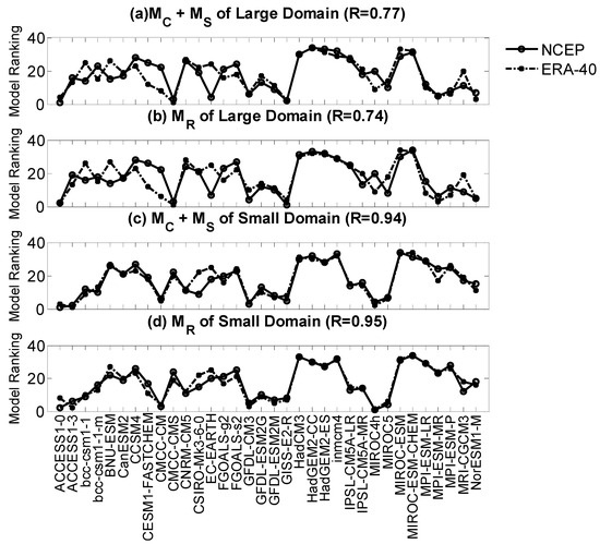
Figure 8.
Comparison of the model ranking from the NCEP and ERA-40: (a) + of large domain, (b) of large domain, (c) + of small domain, and (d) of small domain.
In the large domain, the correlation coefficients for the two ranking results were 0.77 ( + ) and 0.74 (), respectively. Similarly, in the small domain, a significant correlation (at the 95% confidence level) was observed with correlation coefficients of 0.94 ( + ) and 0.95 (). To ensure robustness in the pattern ranking results, we considered both reanalysis data as references.
Our analysis revealed notable differences in the correlation coefficients between the large and small domains. Specifically, the correlation coefficients were significantly smaller for the large domain compared to the small domain. Additionally, a higher number of changes in the model ranking order were observed in the large domain, with at least eight instances of such changes. In contrast, the smaller domains exhibited a much lower number of ranking changes, with approximately three instances occurring. These findings suggest that certain portions of the model’s simulation capability tend to be more unstable as the study area expands.
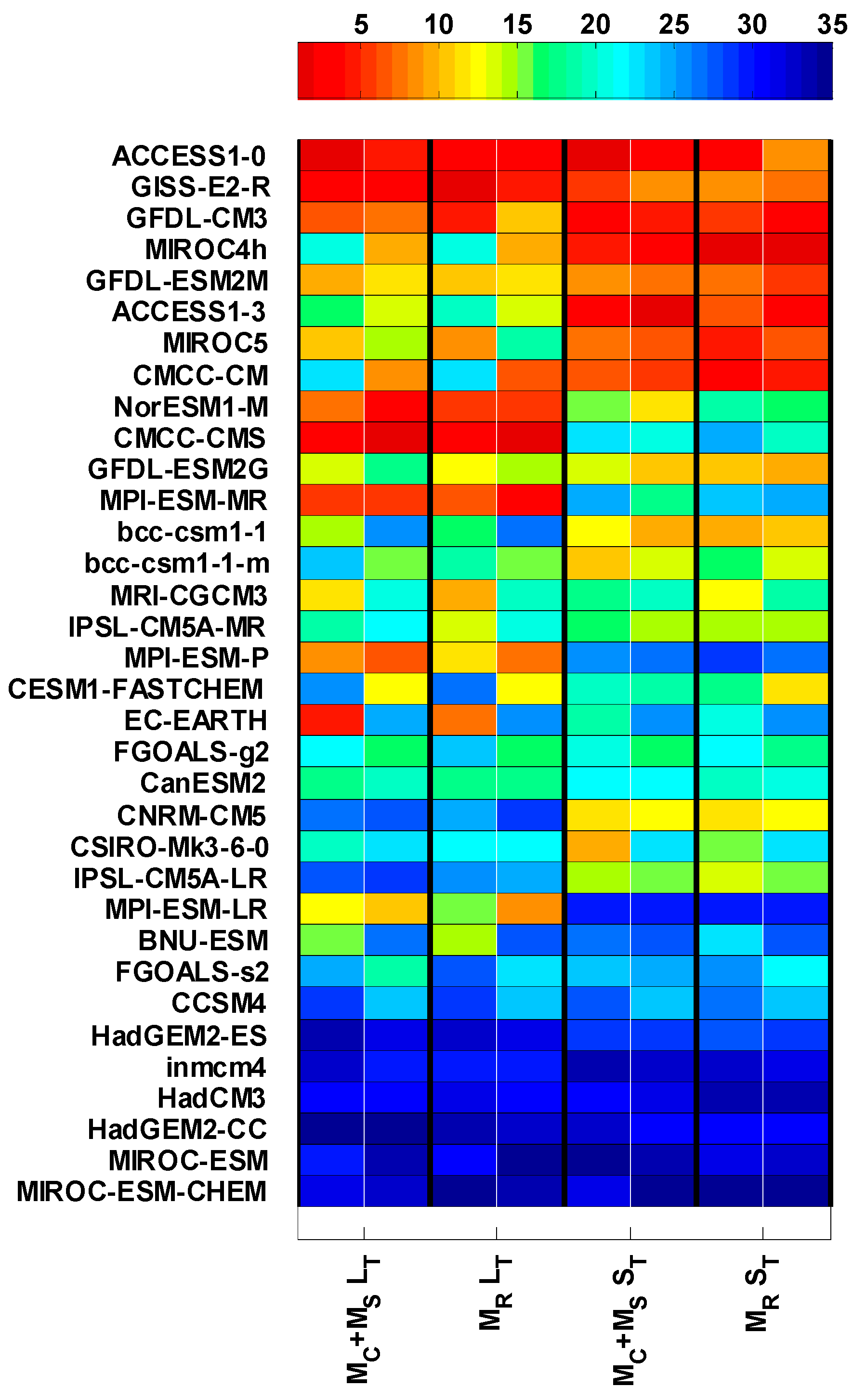
4.3.4. Model Ranking across All Measures
Figure 9 depicts the model ranking derived from a comprehensive set of evaluation measures used in this study. These measures were assessed using two distinct sets of reanalysis data. The colors assigned to each rank in the figure visually illustrate significant variations in model ranks across the evaluated measures. Certain models consistently achieved high ranks, such as ACCESS1-0 and GISS-E2-R, while others consistently obtained low ranks, including MI-ROC-ESM-CHEM and MIROC-ESM.
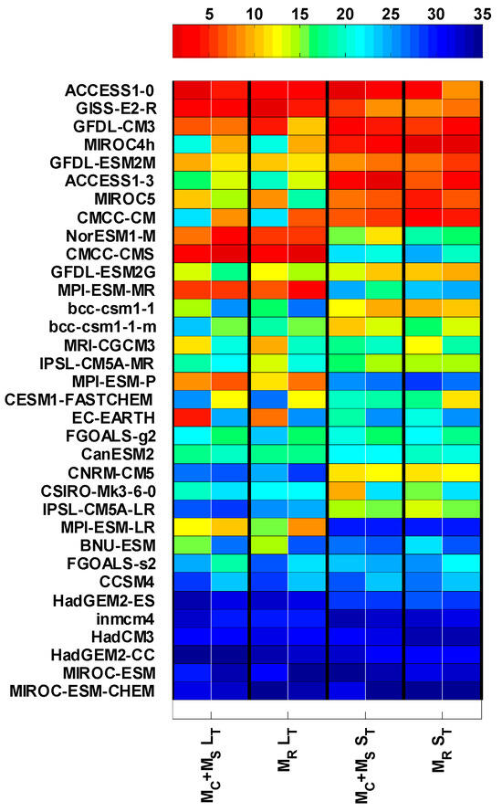
Figure 9.
Ranking of models based on a set of metrics for the small domain (S) and large domain (L). The cells in each square are color-coded to indicate the ranking of the models over the NCEP (left) and ERA-40 (right) datasets. The top-performing model is assigned a rank of 1, while the worst-performing model is assigned a rank of 34.
When considering the cumulative ranks for each model, the top five models identified are ACCESS1-0, GISS-E2-R, GFDL-CM3, MIROC4h, and GFDL-ESM2M.
To emphasize the rankings obtained from the NCEP and ERA-40 reanalysis data, the cells within each square in the figure are color-coded. Our ranking system assigns a rank of 1 to the model with the highest performance and a rank of 34 to the model with the lowest performance. By examining the color pattern in each square, we can discern the relative performance of the models over the two datasets.
This ranking scheme serves as a valuable tool for comparing and contrasting the accuracy and reliability of different models. It allows us to identify models that excel in capturing the characteristics and dynamics of both small and large domains, as well as those that may exhibit shortcomings or inconsistencies.
Such evaluations provide crucial insights into the suitability of models for specific applications or research purposes. They also contribute to ongoing efforts to enhance our understanding of climate patterns and improve the quality of reanalysis data.
It is important to note that these rankings are based solely on the metrics used in this study. Other factors, such as computational efficiency or data availability, should be taken into consideration when selecting a model for practical applications.
Overall, this ranking analysis provides a comprehensive overview of model performance in both small and large domains, shedding light on their strengths and weaknesses.
5. Discussion
The aim of this study is to evaluate the capacity of a model and investigate the impacts of different evaluation metrics, self-organizing map (SOM) size selection, and reanalysis data choice on the assessment of model performance. Our research findings reveal the interrelationships among various evaluation metrics and demonstrate that the choice of evaluation metrics has limited influence on model ranking.
We conducted evaluations of the models’ capabilities using selected evaluation metrics in both small-scale and large-scale spatial domains. Correlation analysis showed significant relationships among different evaluation metrics. We found that the choice of evaluation metrics has only a minor impact on model ranking. We also found that the size of the study area exhibited a positive correlation with model ranking.
To investigate the sensitivity of model ranking to the selection of SOM size, we ranked the models using four different SOM sizes (3 × 3, 4 × 4, 5 × 5, and 6 × 6). The results showed a significant positive correlation among different sizes. Therefore, caution should be taken when selecting the SOM size in the evaluation method.
Furthermore, we compared the results of model evaluation using different reanalysis datasets (NCEP and ERA-40) and found a high consistency in model ranking between the two datasets. The top five models were determined to be ACCESS1-0, GISS-E2-R, GFDL-CM3, MIROC4h, and GFDL-ESM2M based on the evaluation metrics and reanalysis datasets.
Our findings are of great significance for improving the evaluation methods of climate models and enhancing our understanding and prediction of climate change. These findings can serve as a reference for future research. This paper concludes that the choice of evaluation metrics, the size of the study area, and SOM size selection all have certain influences on model ranking.
The classification of weather regimes based on their patterns plays a crucial role in assessing the performance of climate models. Weather regimes are classified according to their distinctive characteristics and temporal evolution. The utilization of these categorized weather patterns in evaluating climate models serves several key purposes:
(a) Firstly, it enhances our comprehension of how climate models perform across diverse weather systems. This tool enables the identification of biases and uncertainties inherent in climate models when simulating various weather system types.
(b) Secondly, it facilitates the assessment of climate models’ capability to accurately simulate extreme weather events. Through classifying extreme weather events into specific weather regimes, we can evaluate the modeling proficiency of climate models for different weather patterns. This evaluation provides invaluable insights into model performance and areas that require improvement.
(c) Thirdly, it contributes to the development and evaluation of ensemble prediction methods. By utilizing the classification of weather regimes, ensemble strategies can be tailored based on the frequency and significance of different patterns. This enables more precise capturing of the full range of variations and uncertainties inherent in different weather systems. Additionally, it allows for an evaluation of the effectiveness of ensemble prediction strategies and identifies potential avenues for further improvements.
In conclusion, the classification of weather regimes and its application in climate model evaluation play a significant role in comprehending model performance, assessing simulations of extreme weather events, and refining ensemble prediction strategies.
6. Summary and Conclusions
The objective of this study was to assess the performance of a model by examining the effects of different evaluation metrics, self-organizing map (SOM) sizes, and reanalysis data choices. Moreover, correlations among various evaluation metrics were explored. The results showed a positive correlation between the size of the study area and observed differences, which was consistent across different evaluation metrics. Among the evaluation metrics used in both large-scale and small-scale spatial domains, the highest correlation coefficient was found between Evaluation Metric and (0.96 for large scale and 0.97 for small scale), while the correlation between Evaluation Metric and was relatively lower (0.79 for large scale and 0.86 for small scale). It can be inferred that the choice of evaluation metrics had a minor impact on model rankings.
Additionally, a significant positive correlation was observed when comparing correlation coefficients calculated for different-sized regions using the same evaluation metrics. Specifically, the correlation coefficients between the three evaluation metrics in the two spatial domains were 0.74, 0.79, and 0.63, respectively. These findings suggest that changes in the size of the study area did not significantly affect the model rankings.
To further investigate the relationship between model performance and different SOM sizes, the models were ranked using various SOM sizes. The results indicated a significant positive correlation, with average correlation coefficients of 0.63 for small-scale and 0.64 for large-scale scenarios.
Furthermore, model rankings were compared using different reanalysis datasets (NCEP and ERA-40), revealing a high level of consistency. Correlation coefficients between the two ranking results were 0.77 and 0.74 for the large-scale scenario and 0.94 and 0.95 for the small-scale scenario. This consistency enhances the reliability of the model rankings.
Considering the different evaluation metrics employed in this study and the impact of two reanalysis datasets on model rankings, significant variations in model rankings were observed. Visualization of the rankings using different colors demonstrated consistent high rankings for models such as ACCESS1-0 and GISS-E2-R, while models like MIROC-ESM-CHEM and MIROC-ESM consistently ranked lower. The top five models based on cumulative rankings were determined to be ACCESS1-0, GISS-E2-R, GFDL-CM3, MIROC4h, and GFDL-ESM2M.
In conclusion, the choice of evaluation metrics, SOM sizes, and reanalysis data selection exerted influence on model performance assessments. Different spatial domain sizes may lead to variations in model rankings, while SOM size and reanalysis data selection play a role in the consistency and stability of these rankings. These findings hold great significance for optimizing and enhancing climate model evaluation methods. This study underscores the impact of factors such as evaluation metric choice, study area size, and SOM size on model rankings, providing valuable insights for future research.
Author Contributions
Conceptualization, Y.W.; project administration, Y.W.; supervision, X.S.; validation, Y.W.; writing—original draft, X.S.; writing—review and editing, Y.W. All authors have read and agreed to the published version of the manuscript.
Funding
This study was supported by Science Foundation of Nanjing University of Information Science & Technology, Grant No. 20100077.
Institutional Review Board Statement
Not applicable.
Informed Consent Statement
Not applicable.
Data Availability Statement
The NCEP/NCAR data were provided by the NOAA-CIRES Climate Diagnostics Center, Boulder, Colorado, USA (http://www.cdc.noaa.gov, accessed on 10 August 2019). We would like to express our sincere gratitude to the European Centre for Medium-Range Weather Forecasts (ECMWF) for generously providing the ERA-40 reanalysis data (https://www.ecmwf.int, accessed on 10 August 2019), which have been instrumental in supporting and enhancing our research. The set of gridded precipitation data was provided by Chen et al. (http://rcg.gvc.gu.se/ accessed on 3 September 2021). The outputs of CMIP5 models were derived from the PCMDI (at https://esgf-node.llnl.gov/projects/cmip5, accessed on 3 September 2022).
Acknowledgments
We acknowledge the National Centers for Environmental Prediction of the USA for providing the reanalysis data. We acknowledge the European Centre for Medium-Range Weather Forecasts (ECMWF) for generously providing the ERA-40 reanalysis data. We acknowledge the international modeling groups, the Program for Climate Model Diagnosis and Intercomparison, and the WCRP’s Working Group on Coupled Modeling for their roles in making available the WCRP CMIP5 multi-model datasets. We acknowledge the helpful comments of three anonymous reviewers, who helped to improve this manuscript.
Conflicts of Interest
The authors declare no conflict of interest. The funders had no role in the design of the study; in the collection, analyses, or interpretation of data; in the writing of the manuscript; or in the decision to publish the results.
Abbreviations
SOM—Self-organizing map; CMIP5—Coupled Model Intercomparison Project Phase 5; GCMs—Global Climate Models; REF—Validation data; PTH—The Pacific Subtropical High; TLP—Tropical Low Pressure; MSLP—Mean sea level pressure; PR—Precipitation; NCEP-NCAR—National Center for Environmental Prediction/National Center for Atmospheric Research; ECMWF—European Centre for Medium-Range Weather Forecasts; ERA-40—The 40-year European Centre for Medium-Range Weather Forecasts (ECMWF) Re-Analysis; CHEN05—Gridded precipitation (PR) data provided by Chen et al.; PCMDI—Program for Climate Model Diagnosis & Intercomparison; EPPs—Extreme precipitation patterns; Trained_A—The filtered extreme precipitation data were used as input for training via the Self-Organizing Map (SOM) to obtain the training results; Trained_B—The filtered daily mean sea level pressure (MSLP) data corresponding to extreme precipitation events were used as input, and the Self-Organizing Map (SOM) was employed for training to obtain the training results; PROB_O—Frequency analysis enabled the construction of a two-dimensional binary matrix, where each element represents the probability of a specific circulation pattern being associated with extreme precipitation events. The calculation is based on the analysis of validation data; PROB_M—Frequency analysis enabled the construction of a two-dimensional binary matrix, where each element represents the probability of a specific circulation pattern being associated with extreme precipitation events. The calculation is based on GCMs output data; JJA—The defined summer period includes the months of June, July, and August.
References
- O’Neill, B.C.; Tebaldi, C.; van Vuuren, D.P.; Eyring, V.; Friedlingstein, P.; Hurtt, G.; Knutti, R.; Kriegler, E.; Lamarque, J.-F.; Lowe, J.; et al. The scenario model intercomparison project (ScenarioMIP) for CMIP6. Geosci. Model Dev. 2016, 9, 3461–3482. [Google Scholar] [CrossRef]
- Zhao, L.; Wang, Y.; Zhao, C.; Dong, X.; Yung, Y.L. Compensating Errors in Cloud Radiative and Physical Properties over the Southern Ocean in the CMIP6 Climate Models. Adv. Atmos. Sci. 2022, 39, 2156–2171. [Google Scholar] [CrossRef]
- Song, S.; Yan, X. Evaluation of events of extreme temperature change between neighboring days in CMIP6 models over China. Theor. Appl. Climatol. 2022, 150, 53–72. [Google Scholar] [CrossRef]
- Wei, L.; Xin, X.; Li, Q.; Wu, Y.; Tang, H.; Li, Y.; Yang, B. Simulation and projection of climate extremes in China by multiple Coupled Model Intercomparison Project Phase 6 models. Int. J. Climatol. 2023, 43, 219–239. [Google Scholar] [CrossRef]
- Wang, X.; Pang, G.; Yang, M. Precipitation over the Tibetan Plateau during recent decades: A review based on observations and simulations. Int. J. Climatol. 2018, 38, 1116–1131. [Google Scholar] [CrossRef]
- Masson, D.; Knutti, R. Spatial-scale dependence of climate model performance in the CMIP3 ensemble. J. Clim. 2011, 24, 2680–2692. [Google Scholar] [CrossRef]
- Post, P.; Truija, V.; Tuulik, J. Circulation weather types and their influence on temperature and precipitation in Estonia. Boreal. Environ. Res. 2002, 7, 281–289. [Google Scholar]
- Riediger, U.; Gratzkil, A. Future weather types and their influence on mean and extreme climate indices for precipitation and temperature in Central Europe. Meteorol. Z. 2014, 23, 231–252. [Google Scholar] [CrossRef] [PubMed]
- Lu, K.; Arshad, M.; Ma, X.; Ullah, I.; Wang, J.; Shao, W. Evaluating observed and future spatiotemporal changes in precipitation and temperature across China based on CMIP6-GCMs. Int. J. Climatol. 2022, 42, 7703–7729. [Google Scholar] [CrossRef]
- Cardell, M.F.; Amengual, A.; Romero, R.; Ramis, C. Future extremes of temperature and precipitation in Europe derived from a combination of dynamical and statistical approaches. Int. J. Climatol. 2020, 40, 4800–4827. [Google Scholar] [CrossRef]
- Gleckler, P.J.; Doutriaux, C.; Durack, P.J.; Taylor, K.E.; Zhang, Y.; Williams, D.N.; Mason, E.; Servonnat, J. A More Powerful Reality Test for Climate Models. Eos Trans. Am. Geophys. Union 2020, 101. [Google Scholar] [CrossRef]
- Yazdandoost, F.; Moradian, S.; Izadi, A.; Aghakouchak, A. Evaluation of CMIP6 precipitation simulations across different climatic zones: Uncertainty and model intercomparison. Atmos. Res. 2021, 250, 105369. [Google Scholar] [CrossRef]
- Barnes, E.A. Revisiting the evidence linking Arctic amplification to extreme weather in midlatitudes. Geophys. Res. Lett. 2013, 40, 4734–4739. [Google Scholar] [CrossRef]
- Fernandez-Granja, J.A.; Casanueva, A.; Bedia, J.; Fernandez, J. Improved atmospheric circulation over Europe by the new generation of CMIP6 earth system models. Clim. Dyn. 2021, 56, 3527–3540. [Google Scholar] [CrossRef]
- Hulme, M. Attributing weather extremes to ‘climate change’ A review. Prog. Phys. Geogr. 2014, 38, 499–511. [Google Scholar] [CrossRef]
- Catto, J.L. Extratropical cyclone classification and its use in climate studies. Rev. Geophys. 2016, 54, 486–520. [Google Scholar] [CrossRef]
- Sousa, P.M.; Trigo, R.M.; Barriopedro, D.; Soares, P.M.M.; Ramos, A.M.; Liberato, M.L.R. Responses of European precipitation distributions and regimes to different blocking locations. Clim. Dyn. 2017, 48, 1141–1160. [Google Scholar] [CrossRef]
- Hsu, L.-H.; Wu, Y.-C.; Chiang, C.-C.; Chu, J.-L.; Yu, Y.-C.; Wang, A.-H.; Jou, B.J.-D. Analysis of the Interdecadal and Interannual Variability of Autumn Extreme Rainfall in Taiwan Using a Deep-Learning-Based Weather Typing Approach. Asia-Pac. J. Atmos. Sci. 2023, 59, 185–205. [Google Scholar] [CrossRef]
- Christensen, H.M.; Moroz, I.M.; Palmer, T.N. Simulating weather regimes: Impact of stochastic and perturbed parameter schemes in a simple atmospheric model. Clim. Dyn. 2015, 44, 2195–2214. [Google Scholar] [CrossRef]
- Huth, R. A circulation classification scheme applicable in GCM studies. Theor. Appl. Climatol. 2000, 67, 1–18. [Google Scholar] [CrossRef]
- Lorenzo, M.N.; Ramos, A.M.; Taboada, J.J.; Gimeno, L. Changes in present and future circulation types frequency in northwest Iberian Peninsula. PLoS ONE 2011, 6, e16201. [Google Scholar] [CrossRef] [PubMed]
- Stryhal, J.; Plavcová, E. On using self-organizing maps and discretized Sammon maps to study links between atmospheric circulation and weather extremes. Int. J. Climatol. 2023, 43, 2678–2698. [Google Scholar] [CrossRef]
- Gibson, P.B.; Perkins-Kirkpatrick, S.E.; Uotila, P.; Pepler, A.S.; Alexander, L.V. On the use of self-organizing maps for studying climate extremes. J. Geophys. Res. Atmos. 2017, 122, 3891–3903. [Google Scholar] [CrossRef]
- Wang, Y.; Jiang, Z.; Chen, W. Performance of CMIP5 models in the simulation of climate characteristics of synoptic patterns over East Asia. J. Meteorol. Res. 2015, 29, 594–607. [Google Scholar] [CrossRef]
- Gibson, P.B.; Uotila, P.; Perkins-Kirkpatrick, S.E.; Alexander, L.V.; Pitman, A.J. Evaluating synoptic systems in the CMIP5 climate models over the Australian region. Clim. Dyn. 2016, 47, 2235–2251. [Google Scholar] [CrossRef]
- Li, M.; Jiang, Z.; Zhou, P.; Le Treut, H.; Li, L. Projection and possible causes of summer precipitation in eastern China using self-organizing map. Clim. Dyn. 2020, 54, 2815–2830. [Google Scholar] [CrossRef]
- Gore, M.J.; Zarzycki, C.M.; Gervais, M.M. Connecting Large-Scale Meteorological Patterns to Extratropical Cyclones in CMIP6 Climate Models Using Self-Organizing Maps. Earth's Future 2023, 11, e2022EF003211. [Google Scholar] [CrossRef]
- Jaye, A.B.; Bruyère, C.L.; Done, J.M. Understanding future changes in tropical cyclogenesis using Self-Organizing Maps. Weather Clim. Extremes 2019, 26, 100235. [Google Scholar] [CrossRef]
- Harrington, L.J.; Gibson, P.B.; Dean, S.M.; Mitchell, D.; Rosier, S.M.; Frame, D.J. Investigating event-specific drought attribution using self-organizing maps. J. Geophys. Res. Atmos. 2016, 121, 12766–12780. [Google Scholar] [CrossRef]
- Yu, T.; Chen, W.; Gong, H.; Feng, J.; Chen, S. Comparisons between CMIP5 and CMIP6 models in simulations of the climatology and interannual variability of the east asian summer Monsoon. Clim. Dyn. 2023, 60, 2183–2198. [Google Scholar] [CrossRef]
- Bu, L.; Zuo, Z.; An, N. Evaluating boreal summer circulation patterns of CMIP6 climate models over the Asian region. Clim. Dyn. 2021, 58, 427–441. [Google Scholar] [CrossRef]
- Guan, W.; Hu, H.; Ren, X.; Yang, X.-Q. Subseasonal zonal variability of the western Pacific subtropical high in summer: Climate impacts and underlying mechanisms. Clim. Dyn. 2019, 53, 3325–3344. [Google Scholar] [CrossRef]
- Ha, K.-J.; Seo, Y.-W.; Lee, J.-Y.; Kripalani, R.H.; Yun, K.-S. Linkages between the South and East Asian summer monsoons: A review and revisit. Clim. Dyn. 2018, 51, 4207–4227. [Google Scholar] [CrossRef]
- Huang, Y.; Wang, B.; Li, X.; Wang, H. Changes in the influence of the western Pacific subtropical high on Asian summer monsoon rainfall in the late 1990s. Clim. Dyn. 2018, 51, 443–455. [Google Scholar] [CrossRef]
- Wang, C.; Zhang, L.; Wu, G. Pacific-East Asian Teleconnection: How Does ENSO Affect East Asian Climate? J. Clim. 2013, 26, 990–1002. [Google Scholar] [CrossRef]
- Wang, G.; Zhang, Q.; Yu, H.; Shen, Z.; Sun, P. Double increase in precipitation extremes across China in a 1.5 °C/2.0 °C warmer climate. Sci. Total Environ. 2020, 746, 140807. [Google Scholar] [CrossRef] [PubMed]
- Wang, J.; Chen, F.; Doan, Q.-V.; Xu, Y. Exploring the effect of urbanization on hourly extreme rainfall over Yangtze River Delta of China. Urban Clim. 2021, 36, 100781. [Google Scholar] [CrossRef]
- Wang, Q.-X.; Wang, M.-B.; Fan, X.-H.; Zhang, F.; Zhu, S.-Z.; Zhao, T.-L. Trends of temperature and precipitation extremes in the Loess Plateau Region of China, 1961–2010. Theor. Appl. Climatol. 2017, 129, 949–963. [Google Scholar] [CrossRef]
- Pérez, J.; Menendez, M.; Mendez, F.; Losada, I. Evaluating the performance of CMIP3 and CMIP5 global climate models over the north–east Atlantic region. Clim. Dyn. 2014, 43, 2663–2680. [Google Scholar] [CrossRef]
- Kalnay, E.; Kanamitsu, M.; Kistler, R.; Collins, W.; Deaven, D.; Gandin, L.; Iredell, M.; Saha, S.; White, G.; Woollen, J.; et al. The NCAR/NCAR 40-year reanalysis project. Bull. Am. Meteorol. Soc. 1996, 77, 437–471. [Google Scholar] [CrossRef]
- Uppala, S.M.; Kallberg, P.W.; Simmons, A.J. The ERA-40 Reanalysis. Q. J. R. Meteorol. Soc. 2005, 131, 2961–3012. [Google Scholar] [CrossRef]
- Gleckler, P.J.; Taylor, K.E.; Doutriaux, C. Performance metrics for climate models. J. Geophys. Res. 2008, 113, L06711. [Google Scholar] [CrossRef]
- Chen, D.; Ou, T.; Gong, L.; Xu, C.Y.; Li, W.; Ho, C.H.; Qian, W. Spatial interpolation of daily precipitation in China: 1951–2005. Adv. Atmos. Sci. 2010, 27, 1221–1232. [Google Scholar] [CrossRef]
- Taylor, K.E.; Stouffer, R.J.; Meehl, G.A. An overview of CMIP5 and the experiment design. Bull. Am. Meteorol. Soc. 2012, 93, 485–498. [Google Scholar] [CrossRef]
- Kohonen, T. Self-organized formation of topologically correct feature maps. Biol. Cybern. 1982, 43, 59–69. [Google Scholar]
- Zhao, S.; Deng, Y.; Black, R.X. A Dynamical and Statistical Characterization of U.S. Extreme Precipitation Events and Their Associated Large-Scale Meteorological Patterns. J. Clim. 2017, 30, 1307–1326. [Google Scholar] [CrossRef]
- Radić, V.; Clarke, G.K.C. Evaluation of IPCC models’ performance in simulating late-twentieth-century climatologies and weather patterns over North America. J. Clim. 2011, 24, 5257–5274. [Google Scholar]
- Schuenemann, K.C.; Cassano, J.J. Changes in synoptic weather patterns and Greenland precipitation in the 20th and 21st centuries: 2. Analysis of 21st century atmospheric changes using self-organizing maps. J. Geophys. Res. 2009, 115, D05108. [Google Scholar] [CrossRef]

Disclaimer/Publisher’s Note: The statements, opinions and data contained in all publications are solely those of the individual author(s) and contributor(s) and not of MDPI and/or the editor(s). MDPI and/or the editor(s) disclaim responsibility for any injury to people or property resulting from any ideas, methods, instructions or products referred to in the content. |
© 2023 by the authors. Licensee MDPI, Basel, Switzerland. This article is an open access article distributed under the terms and conditions of the Creative Commons Attribution (CC BY) license (https://creativecommons.org/licenses/by/4.0/).