

Evaluation of Rain Estimates from Several Ground-Based Radar Networks and Satellite Products for Two Cases Observed over France in 2022

Abstract
:1. Introduction
2. Materials and Methods
2.1. Description of the Precipitation Products
2.1.1. RADOME Rain Gauges Network
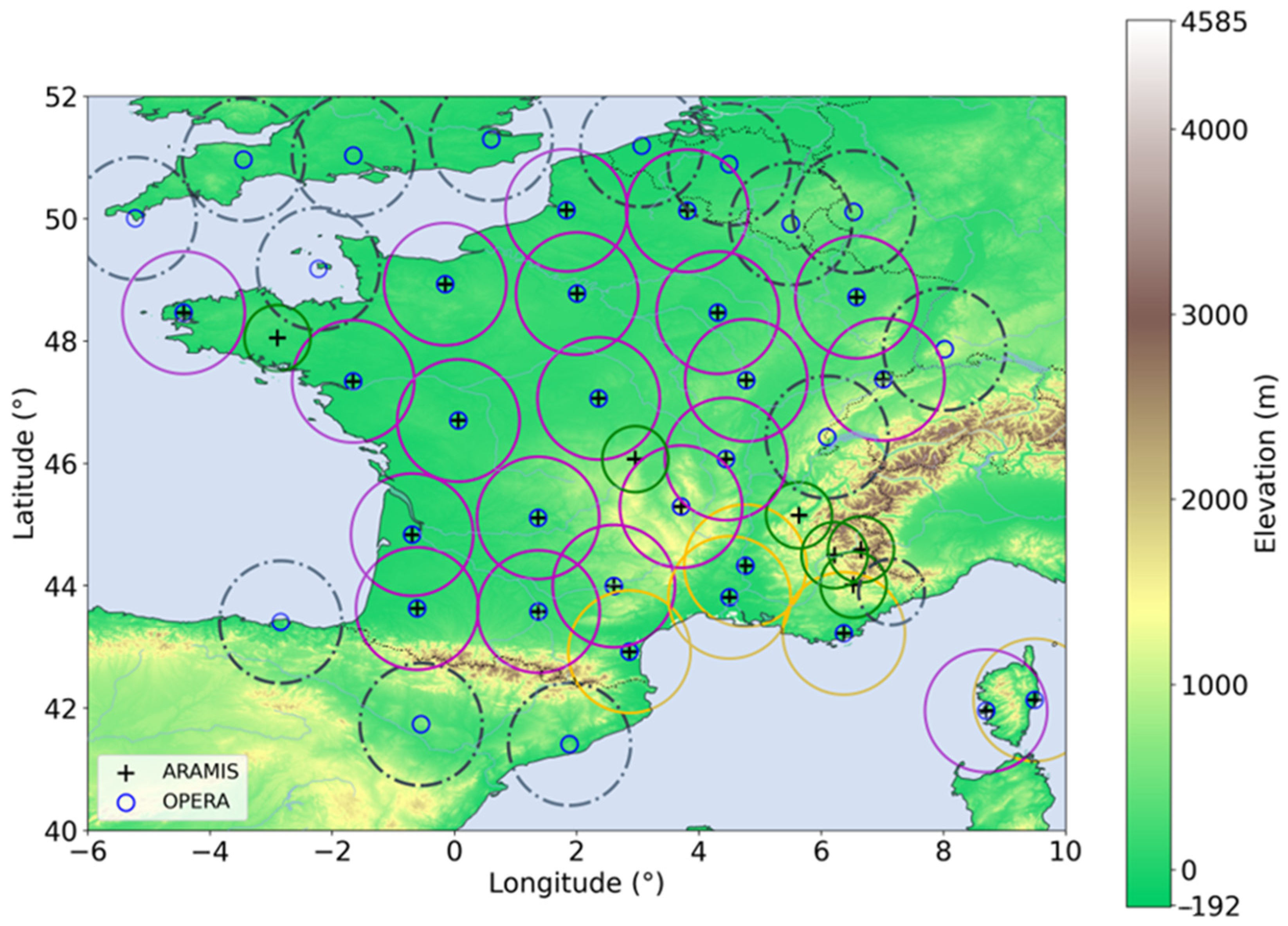
2.1.2. Radar Networks
- A ground-clutter identification by using pulse-to-pulse fluctuation of the radar reflectivity with further analysis for pixels adjacent to an identified clutter pixel;
- Non-meteorological echoes and precipitation-attenuation corrections from polarimetric modules;
- A partial beam-blockage correction by numerically simulating the interaction between the radar wave propagation and the ground by using orographic maps and long-term precipitation accumulation to identify trees and anthropogenic structures;
- A vertical profile of reflectivity correction deriving from ratios of hourly rainfall accumulation at different elevation angles and using these ratios to determine an optimal vertical profile reflectivity scheme from a predefined set;
- A gas-attenuation correction depending on the wavelength used and the altitude above the sea level;
- The synchronization or correction for advection;
- A weighted linear combination of the corrected reflectivity measurement at different elevation;
- The reflectivity (Z) conversion to rain rate (R) by using the Z-R relationship Z = 200 · R1.6, the 5 min rainfall accumulation;
- The rain-gauge adjustment.
- An anomaly-removal module identifying non-weather-related pixels;
- A hit-accumulation clutter filter which detects pixels with an occurrence frequency higher than a reference threshold of 0.6;
- A beam-blockage correction;
- A satellite-based filter of residual non-rain echoes from the probability of the Precipitation Clouds product of the EUMETSAT Nowcasting Satellite Application Facilities.
- The differences between the radars in the network;
- The contamination by non-meteorological targets (partially corrected as explained earlier and in [28] with the implementation of a hit-accumulation clutter);
- The absence of correction of the vertical profile of reflectivity of the raw scans;
- The use of the single Marshall-Palmer relationship to convert Z to R.
2.1.3. Satellite Precipitation Products
IR Sensor-Based Satellite Products
- A better identification of warmer stratiform clouds from higher temperature thresholds;
- An improvement in the watershed method used for the image segmentation;
- An improvement in the rainfall regime identification by adding monthly sets of cloud types to the existing cloud classification system;
- The use of PMW satellite data to adjust Tb–R curves;
Microwave Sensor-Based and Blended Products
- IMERG-Early (later called EARLY) is the earliest version of the IMERG product available after nominal observation; with approximately 4 h of data latency, the propagation of precipitation fields determined by the observation of IR sensors is applied only forward in time;
- IMERG-Late version (later called LATE) is available after a latency of 14 h and has its precipitation fields propagated forward and backward in time.
Carrier-to-Noise-Based Precipitation Product
2.2. Point-to-Pixel Comparative Method
- Geostatistical methods (e.g., the different Kriging methods; [58]).
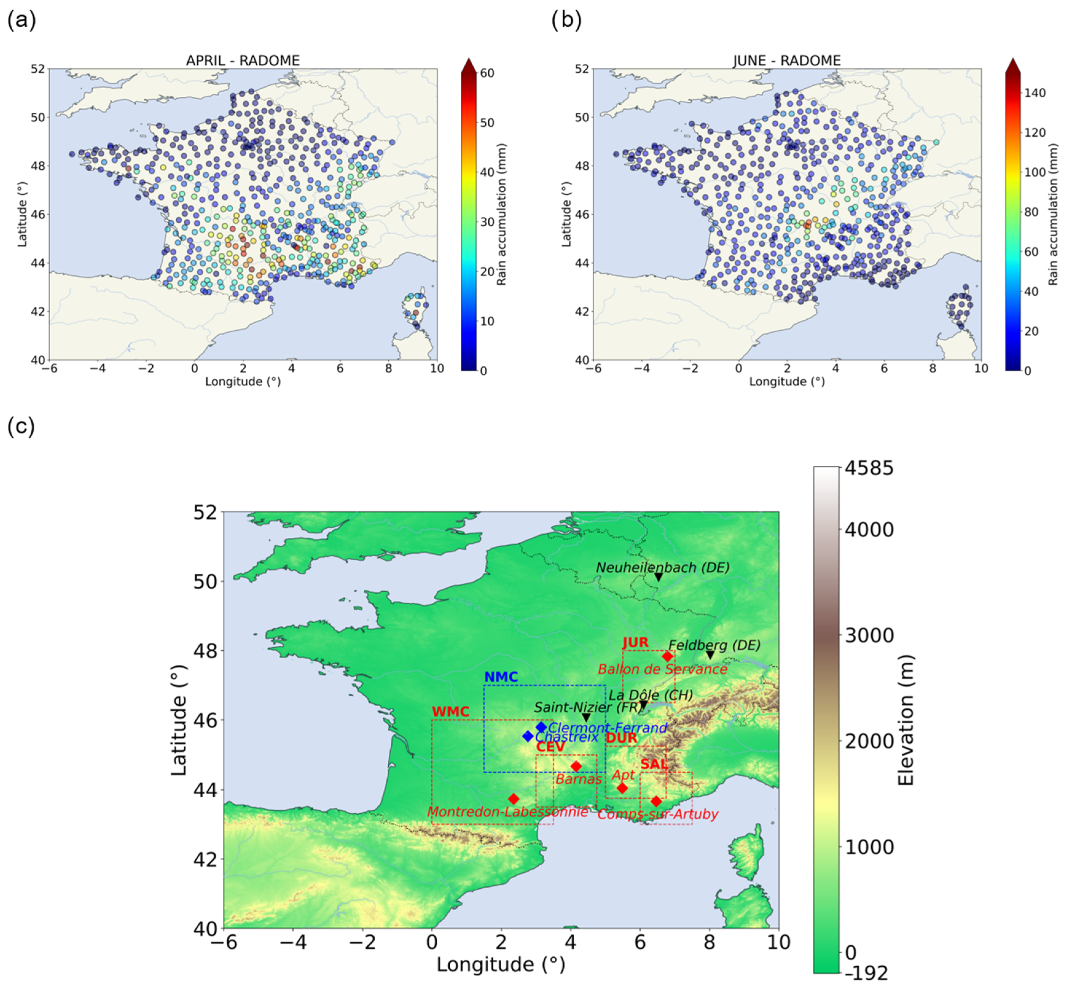
2.3. Synoptic Description of the Two Case Studies
3. Comparative Analyses Results
3.1. Rain-Gauge vs. Radar Observations
3.1.1. PANTHERE vs. RADOME
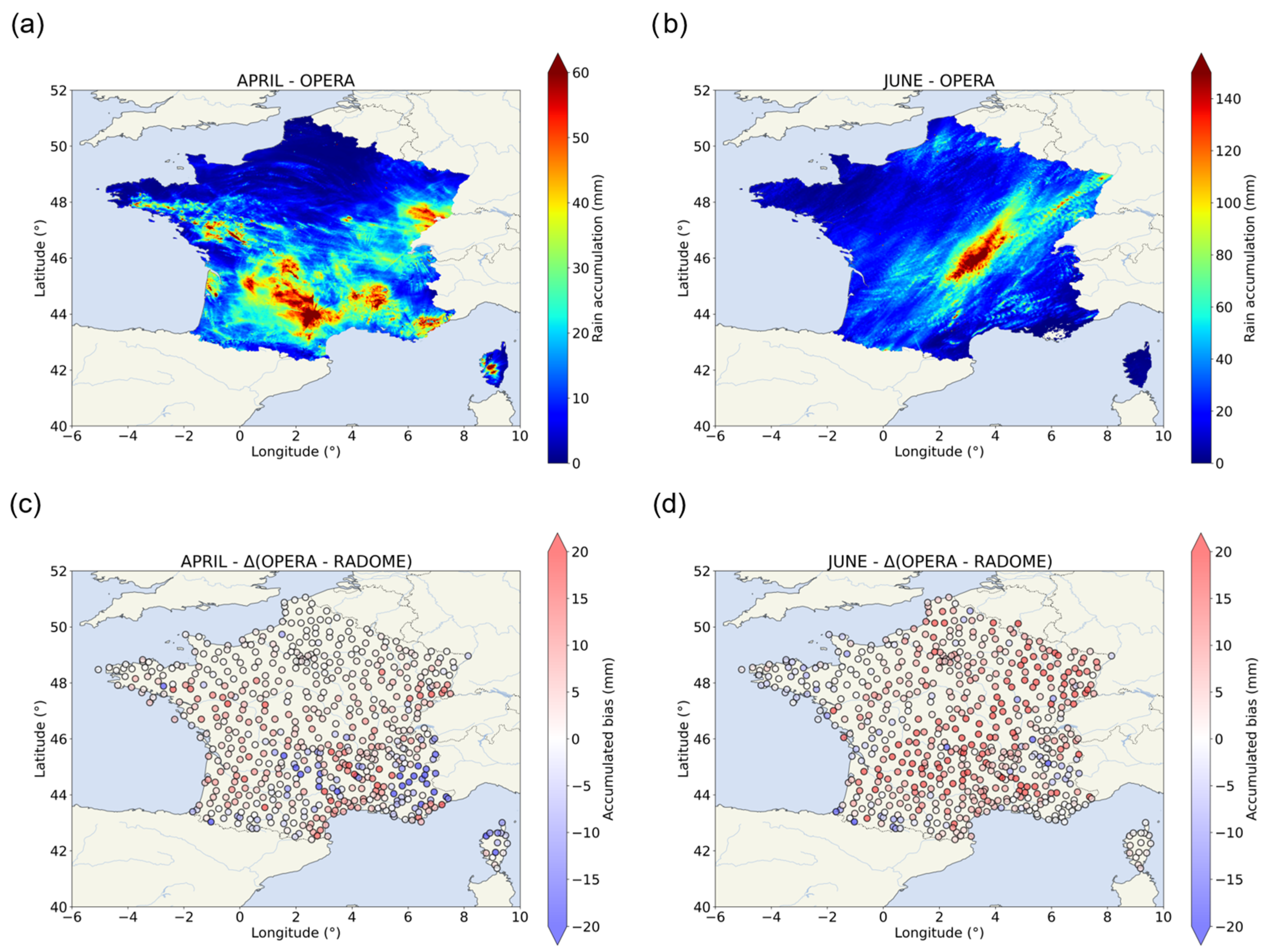
3.1.2. OPERA vs. RADOME
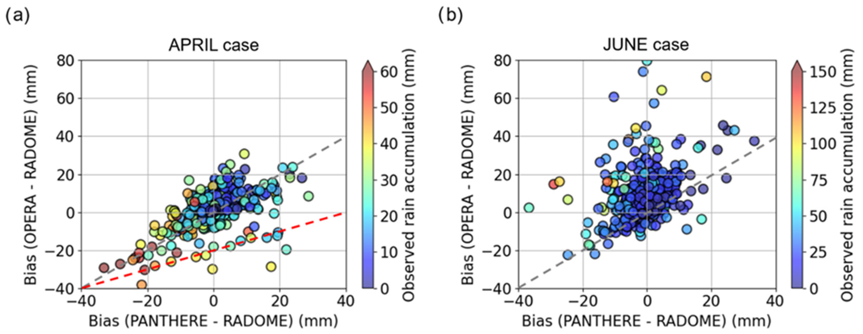
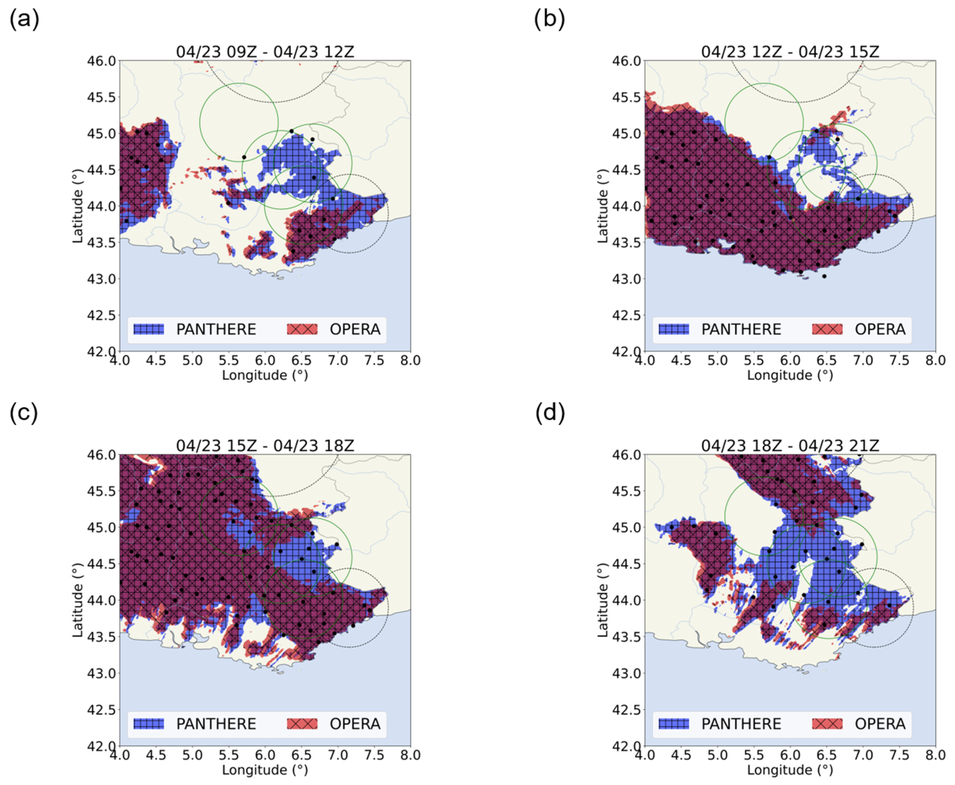
3.1.3. PANTHERE and OPERA vs. RADOME
3.2. Rain-Gauge vs. Satellite Precipitation Products
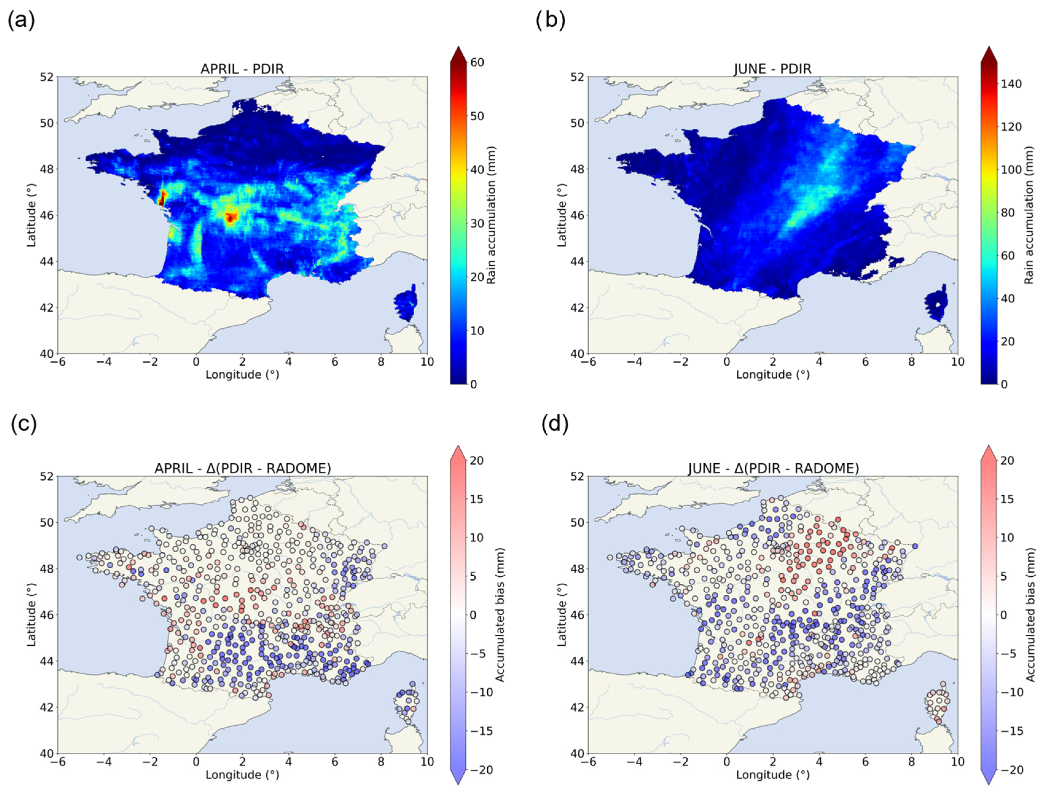
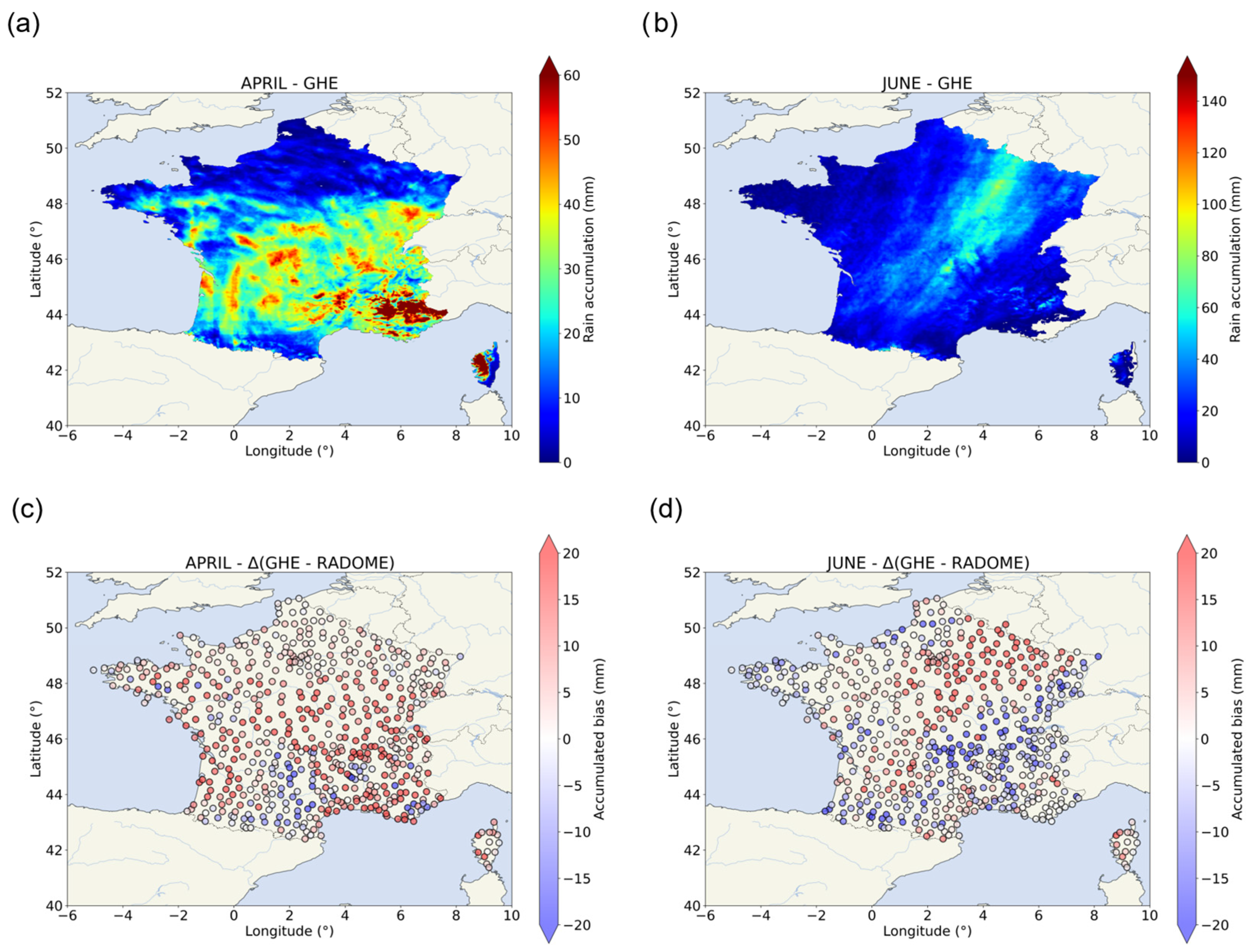
3.2.1. IR Sensor-Based Product
3.2.2. MW Sensor-Based Product
IMERG Products
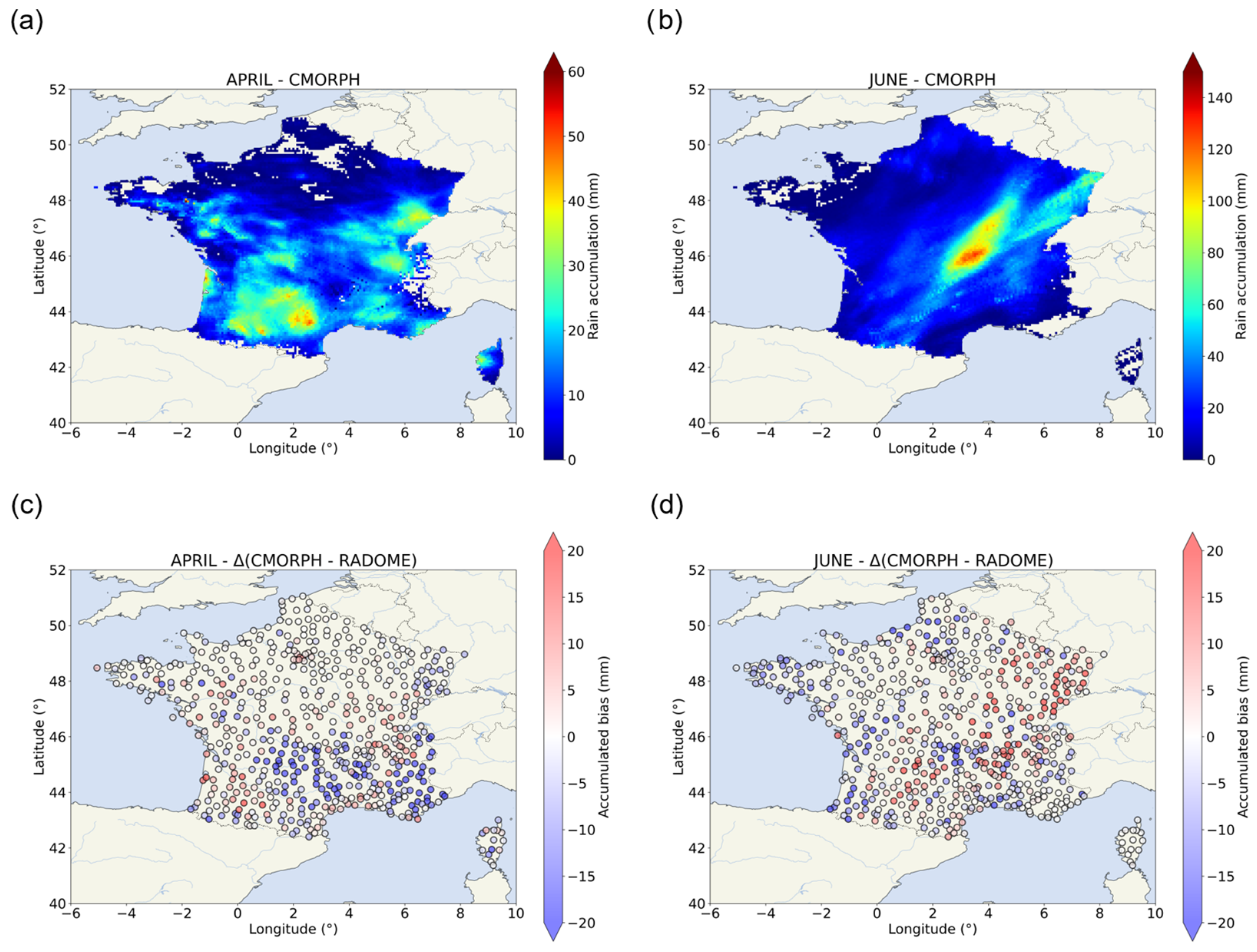
CMORPH Products
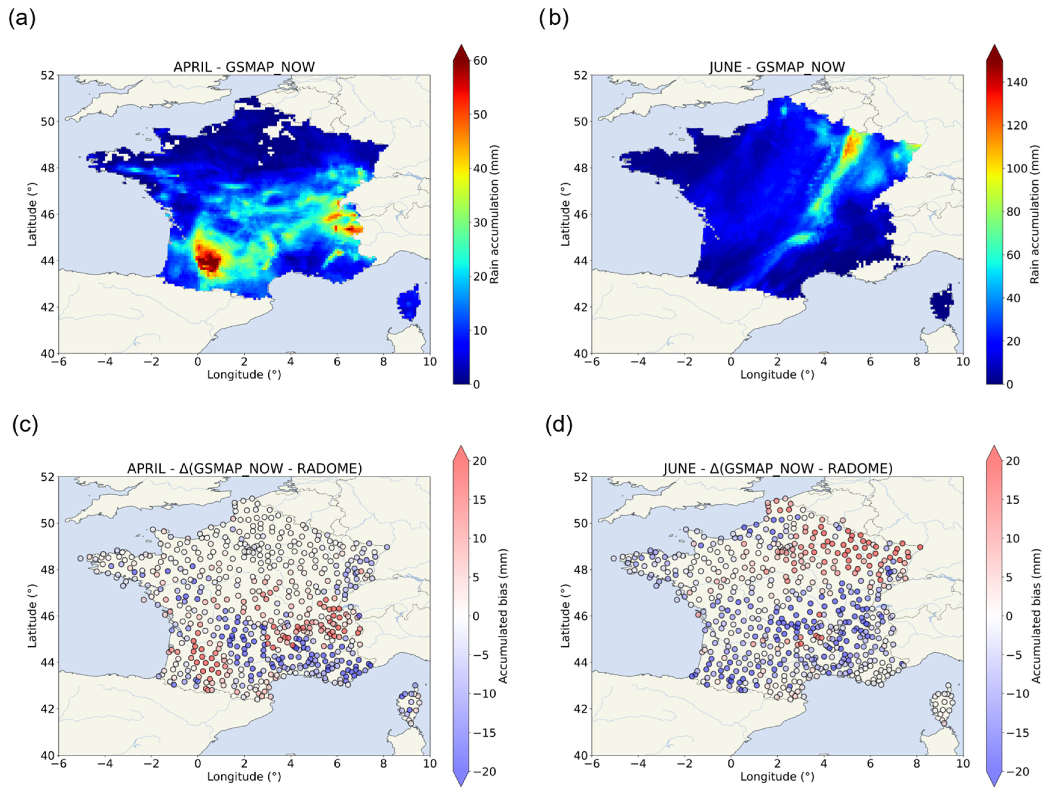
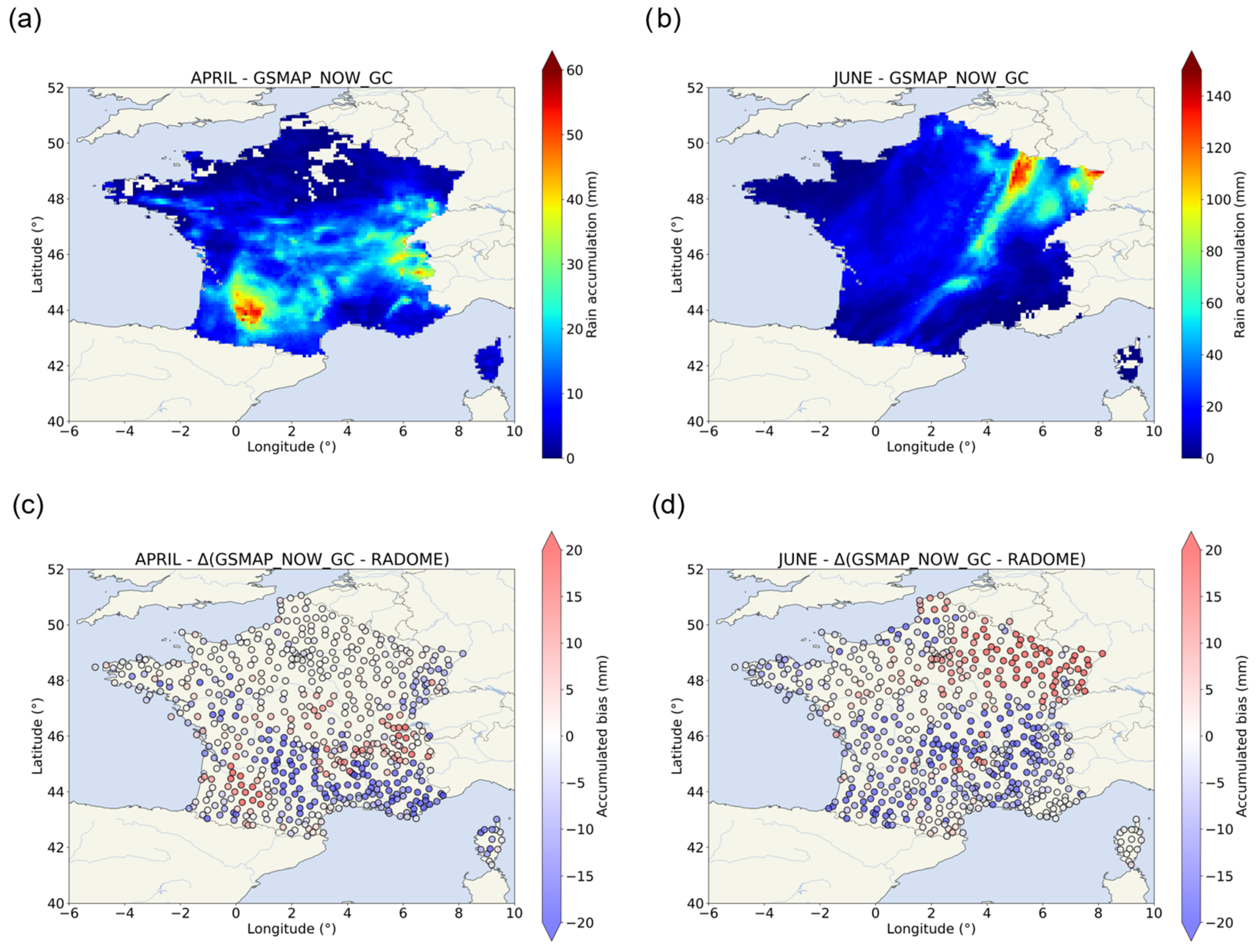
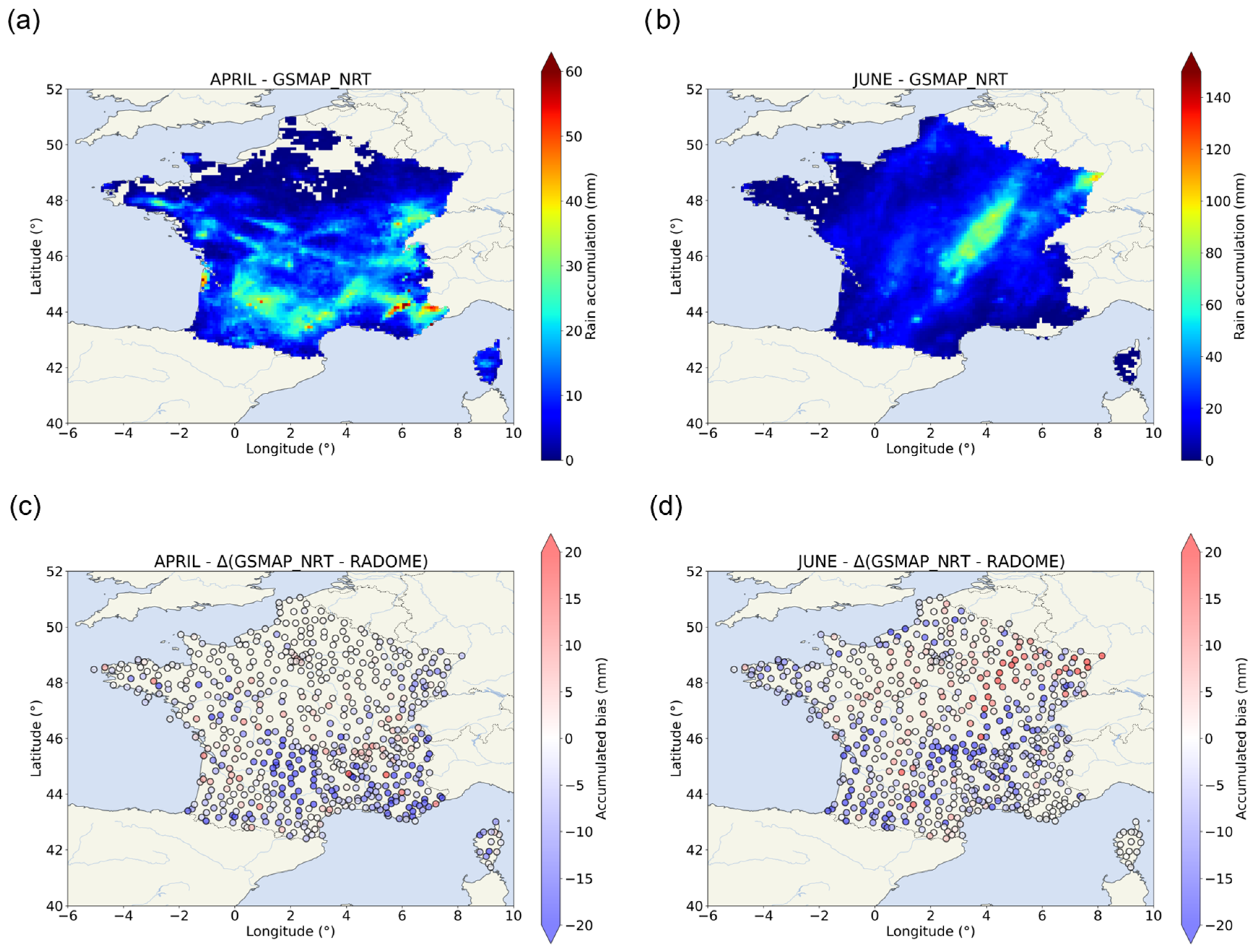
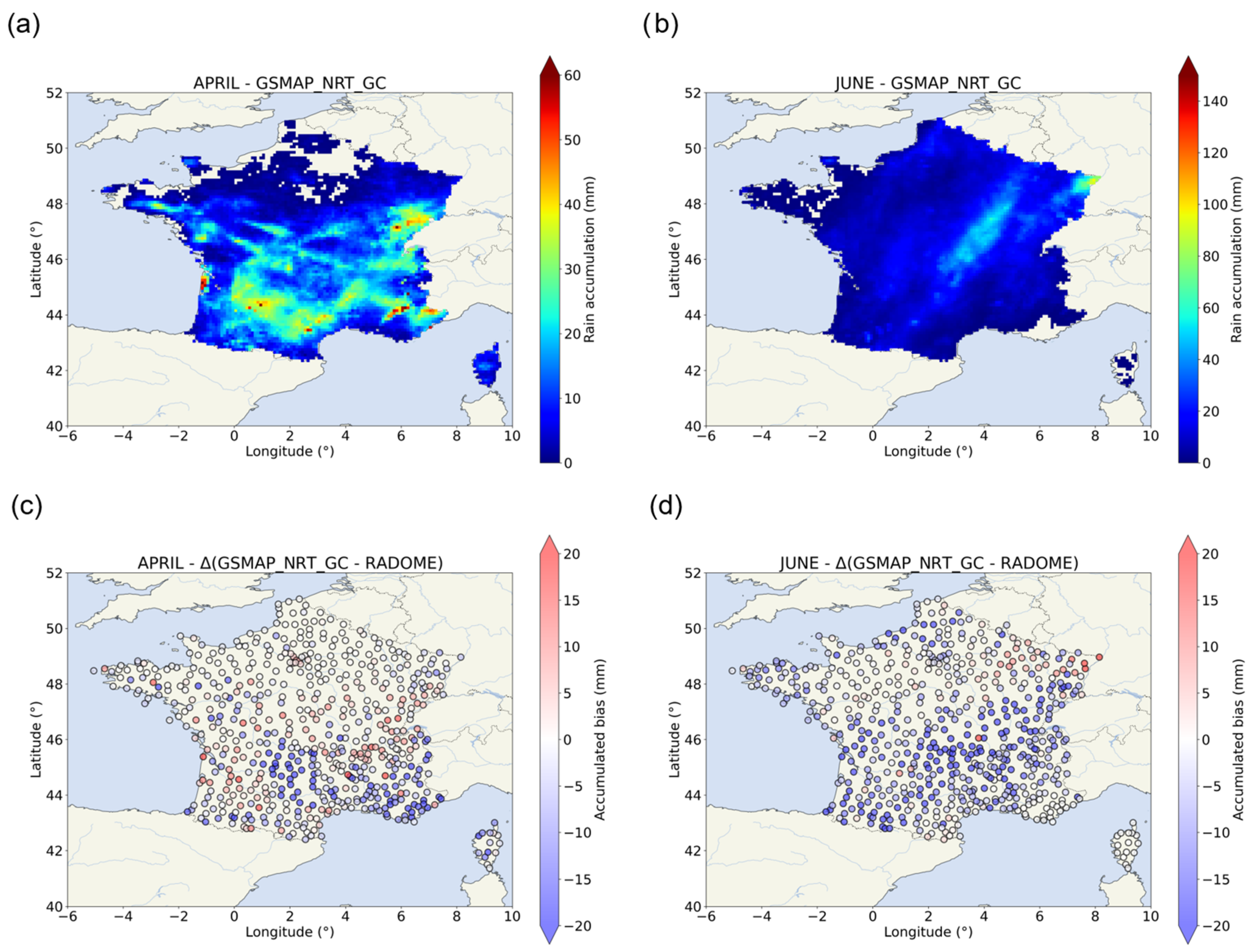
GSMaP Products
3.2.3. C/N-Based Product
4. Discussion
5. Conclusions and Perspectives
- PDIR and GHE found difficulty in identifying the position of the April event but correctly detected the June event. The IR-based technique might be well adapted for these more convective conditions with high spatial (4 × 4 km2) and temporal (15 min to 1 h) resolutions with relatively short latency (minutes to hours);
- Short-latency (real-time) MW-based products tend to produce worse representations of the precipitation cases such as CMORPH-RT and GSMaP-Now products. GSMaP-Now products had difficulty in representing the event but the quantification was coherent with the RADOME observations;
- In comparison, GSMaP-NRT performed better than GSMaP-Now in the detection of the event, especially in the identification of the June event;
- A similar statement can be made about the reprocessed CMORPH version compared to the heterogeneity in precipitation amounts’ quantification by CMORPH-RT. The morphing method allowed for a better representation and quantification of both case studies;
- The gauge-adjustment effectuated for the GSMaP-Now-GC and GSMaP-NRT-GC did not show a significant improvement in the quantification of both events;
- IMERG-Early and IMERG-Late showed a trend to slightly overestimate the presence of rain, as shown by the overestimation recorded at low-rain-amount areas. They also tend to underestimate high rain-rate values but they well represented both case studies over the south regions of France;
- The reprocessing applied to IMERG-Late does not improve the estimations compared to IMERG-Early;
- CMORPH-RT showed traces of raw LEO satellite observation swaths over parts of the country. This was traduced by strong differences at the very-local scale, over the JUR area for example. CMORPH-RT showed low bias medians but CMORPH was better at the spatial representation of both events;
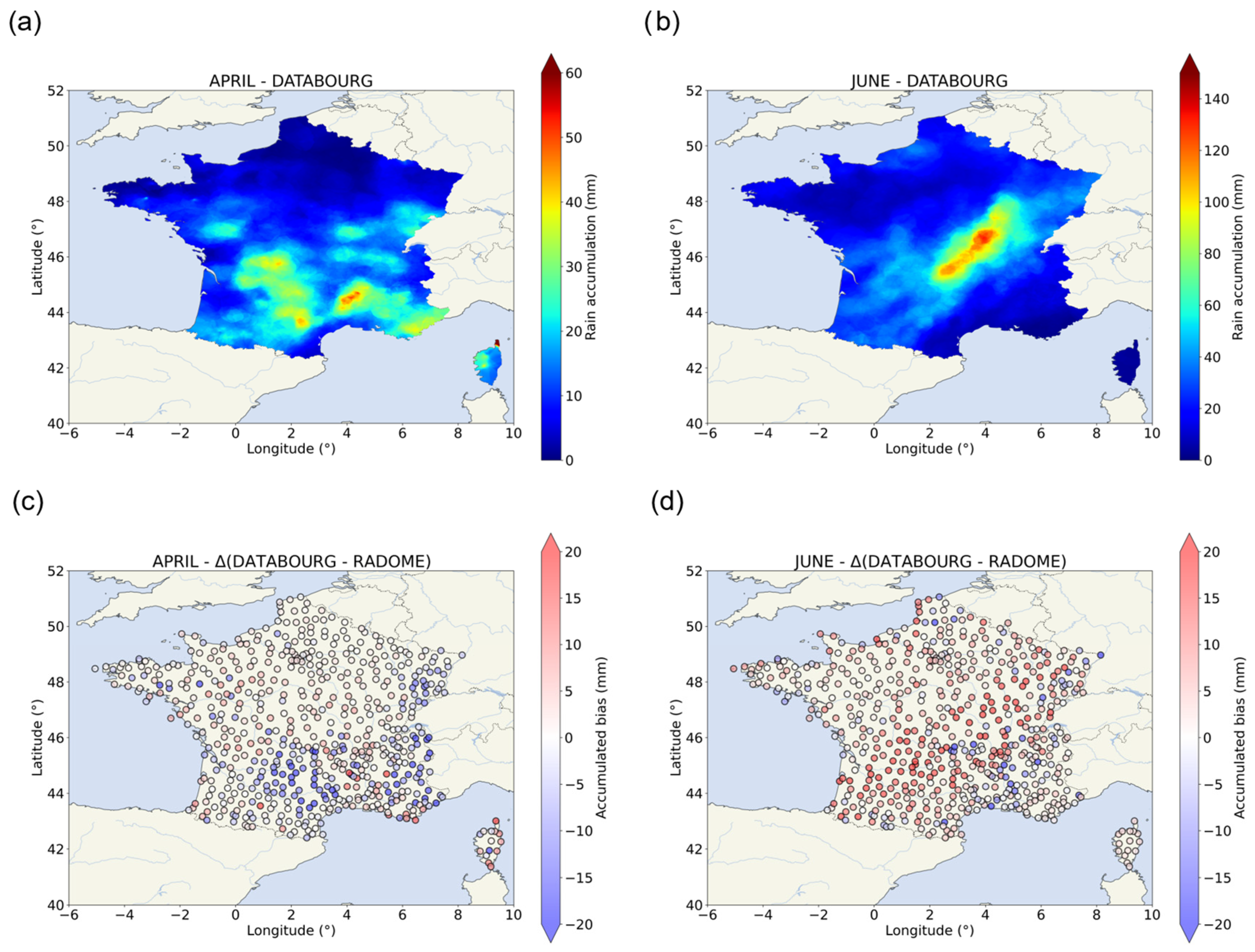
- Despite slightly overestimating during the June event, DATABOURG showed promising results with low biases for both cases with the highest spatiotemporal resolution (1 km2 and 5 min).
Supplementary Materials
Author Contributions
Funding
Institutional Review Board Statement
Informed Consent Statement
Data Availability Statement
Acknowledgments
Conflicts of Interest
Abbreviations
| AMW | Active MicroWave |
| ARAMIS | Application Radar À la Météorologie Infra-Synoptique |
| C/N | Carrier-to-Noise |
| CEV | Cévennes |
| CHRS | Center for Hydrometeorology and Remote Sensing |
| CMORPH | CPC MORPHing |
| CPC | Climate Prediction Center |
| DUR | Durance |
| EUMETNET | European METeorological NETwork |
| GEO | Geostationary Orbit |
| GHE | Global Hydro Estimator |
| GPM | Global Precipitation Measurement |
| GSMaP | Global Satellite Mapping of Precipitation |
| HE | Hydro Estimator |
| IMERG | Integrated Multi-satellitE Retrievals for GPM |
| IPCC | Intergovernmental Panel on Climate Change |
| IR | InfraRed |
| JAXA | Japan Aerospace Exploration Agency |
| JUR | Jura |
| LEO | Low Earth Orbit |
| MW | MicroWave |
| NASA | National Aeronautics and Space Administration |
| NESDIS | National Environmental Satellite, Data and Information Service |
| NMC | Northern Massif Central |
| NOAA | National Oceanic and Atmospheric Administration |
| NRT | Near Real Time |
| OPERA | Operational Program for Exchange of weather RAdar |
| PANTHERE | Projet ARAMIS Nouvelles Technologies en Hydrométéorologie Extension et REnouvellement |
| PCCS | PERSIANN Cloud Classification System |
| PCDR | PERSIANN Climate Data Record |
| PDIR | PERSIANN Dynamic Infrared Rain Rate |
| PERSIANN | Precipitation Estimation from Remotely Sensed Information using Artificial Neural Network |
| PMW | Passive MicroWave |
| R | Rain rate |
| RADOME | Réseau d’Acquisition de Données et d’Observation Météorologiques Etendues |
| RT | Real Time |
| SAL | Southern Alps |
| VPR | Vertical Profile of Reflectivity |
| WMC | Western Massif Central |
| Z | Reflectivity |
References
- Kidd, C.; Huffman, G.; Maggioni, V.; Chambon, P.; Oki, R. The Global Satellite Precipitation Constellation: Current Status and Future Requirements. Bull. Am. Meteorol. Soc. 2021, 102, E1844–E1861. [Google Scholar] [CrossRef]
- Kundzewicz, Z.W.; Kanae, S.; Seneviratne, S.I.; Handmer, J.; Nicholls, N.; Peduzzi, P.; Mechler, R.; Bouwer, L.M.; Arnell, N.; Mach, K.; et al. Flood Risk and Climate Change: Global and Regional Perspectives. Hydrol. Sci. J. 2014, 59, 1–28. [Google Scholar] [CrossRef]
- Volkert, H. Heavy Precipitation in the Alpine Region (HERA): Areal Rainfall Determination for Flood Warnings Through in-Situ Measureme Nts, Remote Sensing and Atmospheric Modelling. Meteorol. Atmos. Phys. 2000, 72, 73–85. [Google Scholar] [CrossRef]
- Vicente-Serrano, S.M.; Beguería, S.; López-Moreno, J.I. A Multiscalar Drought Index Sensitive to Global Warming: The Standardized Precipitation Evapotranspiration Index. J. Clim. 2010, 23, 1696–1718. [Google Scholar] [CrossRef]
- IPCC. Climate Change 2022—Impacts, Adaptation and Vulnerability: Working Group II Contribution to the Sixth Assessment Report of the Intergovernmental Panel on Climate Change; Pörtner, H.-O., Roberts, D.C., Tignor, M., Poloczanska, E.S., Mintenbeck, K., Alegría, A., Craig, M., Langsdorf, S., Löschke, S., Möller, V., et al., Eds.; Cambridge University Press: Cambridge, UK, 2023. [Google Scholar] [CrossRef]
- Ren, M.; Xu, Z.; Pang, B.; Liu, W.; Liu, J.; Du, L.; Wang, R. Assessment of Satellite-Derived Precipitation Products for the Beijing Region. Remote Sens. 2018, 10, 1914. [Google Scholar] [CrossRef]
- Paprotny, D.; Sebastian, A.; Morales-Nápoles, O.; Jonkman, S.N. Trends in Flood Losses in Europe over the Past 150 Years. Nat. Commun. 2018, 9, 1985. [Google Scholar] [CrossRef]
- Cánovas-García, F.; García-Galiano, S.; Alonso-Sarría, F. Assessment of Satellite and Radar Quantitative Precipitation Estimates for Real Time Monitoring of Meteorological Extremes Over the Southeast of the Iberian Peninsula. Remote Sens. 2018, 10, 1023. [Google Scholar] [CrossRef]
- Paranunzio, R.; Chiarle, M.; Laio, F.; Nigrelli, G.; Turconi, L.; Luino, F. New Insights in the Relation between Climate and Slope Failures at High-Elevation Sites. Theor. Appl. Climatol. 2019, 137, 1765–1784. [Google Scholar] [CrossRef]
- Luino, F.; De Graff, J.; Roccati, A.; Biddoccu, M.; Cirio, C.G.; Faccini, F.; Turconi, L. Eighty Years of Data Collected for the Determination of Rainfall Threshold Triggering Shallow Landslides and Mud-Debris Flows in the Alps. Water 2020, 12, 133. [Google Scholar] [CrossRef]
- Kidd, C. Satellite Rainfall Climatology: A Review. Int. J. Climatol. 2001, 21, 1041–1066. [Google Scholar] [CrossRef]
- Sun, Q.; Miao, C.; Duan, Q.; Ashouri, H.; Sorooshian, S.; Hsu, K.-L. A Review of Global Precipitation Data Sets: Data Sources, Estimation, and Intercomparisons. Rev. Geophys. 2018, 56, 79–107. [Google Scholar] [CrossRef]
- du Châtelet, J.P. Aramis, le réseau français de radars pour la surveillance des précipitations. La Météorologie 2003, 40, 44–52. [Google Scholar] [CrossRef]
- Huuskonen, A.; Saltikoff, E.; Holleman, I. The Operational Weather Radar Network in Europe. Bull. Am. Meteorol. Soc. 2014, 95, 897–907. [Google Scholar] [CrossRef]
- Kidd, C.; Levizzani, V. Status of Satellite Precipitation Retrievals. Hydrol. Earth Syst. Sci. 2011, 15, 1109–1116. [Google Scholar] [CrossRef]
- Yu, L.; Leng, G.; Python, A.; Peng, J. A Comprehensive Evaluation of Latest GPM IMERG V06 Early, Late and Final Precipitation Products across China. Remote Sens. 2021, 13, 1208. [Google Scholar] [CrossRef]
- Scofield, R.A.; Kuligowski, R.J. Status and Outlook of Operational Satellite Precipitation Algorithms for Extreme-Precipitation Events. Weather Forecast. 2003, 18, 1037–1051. [Google Scholar] [CrossRef]
- Hsu, K.; Gao, X.; Sorooshian, S.; Gupta, H.V. Precipitation Estimation from Remotely Sensed Information Using Artificial Neural Networks. J. Appl. Meteorol. Climatol. 1997, 36, 1176–1190. [Google Scholar] [CrossRef]
- Joyce, R.J.; Janowiak, J.E.; Arkin, P.A.; Xie, P. CMORPH: A Method That Produces Global Precipitation Estimates from Passive Microwave and Infrared Data at High Spatial and Temporal Resolution. J. Hydrometeorol. 2004, 5, 487–503. [Google Scholar] [CrossRef]
- Kubota, T.; Shige, S.; Hashizume, H.; Aonashi, K.; Takahashi, N.; Seto, S.; Hirose, M.; Takayabu, Y.N.; Ushio, T.; Nakagawa, K.; et al. Global Precipitation Map Using Satellite-Borne Microwave Radiometers by the GSMaP Project: Production and Validation. IEEE Trans. Geosci. Remote Sens. 2007, 45, 2259–2275. [Google Scholar] [CrossRef]
- Huffman, G.J.; Bolvin, D.T.; Braithwaite, D.; Hsu, K.; Joyce, R.; Kidd, C.; Nelkin, E.J.; Sorooshian, S.; Tan, J.; Xie, P. NASA Global Precipitation Easurement (GPM) Integrated Multi-SatellitE Retrievals for GPM (IMERG). NASA Algorithm Theoretical Basis Doc., Version 06, 38p. Available online: https://pmm.nasa.gov/sites/default/files/document_files/IMERG_ATBD_V06.pdf (accessed on 9 October 2023).
- Gharanjik, A.; Mishra, K.V.; Bhavani Shankar, M.R.; Ottersten, B. Learning-Based Rainfall Estimation via Communication Satellite Links. In Proceedings of the 2018 IEEE Statistical Signal Processing Workshop (SSP), Freiburg im Breisgau, Germany, 10–13 June 2018; pp. 130–134. [Google Scholar] [CrossRef]
- Gharanjik, A.; Bhavani Shankar, M.R.B.; Zimmer, F.; Ottersten, B. Centralized Rainfall Estimation Using Carrier to Noise of Satellite Communication Links. IEEE J. Sel. Areas Commun. 2018, 36, 1065–1073. [Google Scholar] [CrossRef]
- Tardieu, J.; Leroy, M. Radome, le réseau temps réel d’observation au sol de Météo-France. La Météorologie 2003, 40, 40–43. [Google Scholar] [CrossRef]
- Guillou, Y. L’automatisation des observations météorologiques de surface à Météo-France. Une r-évolution. La Météorologie 2018, 100, 96–99. [Google Scholar] [CrossRef]
- Tabary, P. The New French Operational Radar Rainfall Product. Part I: Methodology. Weather Forecast. 2007, 22, 393–408. [Google Scholar] [CrossRef]
- Figueras i Ventura, J.; Tabary, P. The New French Operational Polarimetric Radar Rainfall Rate Product. J. Appl. Meteorol. Climatol. 2013, 52, 1817–1835. [Google Scholar] [CrossRef]
- Saltikoff, E.; Haase, G.; Delobbe, L.; Gaussiat, N.; Martet, M.; Idziorek, D.; Leijnse, H.; Novák, P.; Lukach, M.; Stephan, K. OPERA the Radar Project. Atmosphere 2019, 10, 320. [Google Scholar] [CrossRef]
- Le Bastard, T.; Caumont, O.; Gaussiat, N.; Karbou, F. Combined Use of Volume Radar Observations and High-Resolution Numerical Weather Predictions to Estimate Precipitation at the Ground: Methodology and Proof of Concept. Atmos. Meas. Tech. 2019, 12, 5669–5684. [Google Scholar] [CrossRef]
- Chochon, R.; Martin, N.; Lebourg, T.; Vidal, M. Analysis of Extreme Precipitation during the Mediterranean Event Associated with the Alex Storm in the Alpes-Maritimes: Atmospheric Mechanisms and Resulting Rainfall. In Proceedings of the SimHydro 2021: Models for Complex and Global Water Issues, Nice, France, 16–18 June 2021; Available online: https://hal.science/hal-03374712 (accessed on 9 October 2023).
- Qiu, Y. Multiscale Assessment of Hydrological Responses of Nature-Based Solutions to Improve Urban Resilience. Ph.D. Thesis, École des Ponts ParisTech, Champs-sur-Marne, France, 2021. Available online: https://pastel.hal.science/tel-03404617 (accessed on 9 October 2023).
- Park, S.; Berenguer, M.; Sempere-Torres, D. Long-Term Analysis of Gauge-Adjusted Radar Rainfall Accumulations at European Scale. J. Hydrol. 2019, 573, 768–777. [Google Scholar] [CrossRef]
- Nguyen, P.; Shearer, E.J.; Ombadi, M.; Afzali Gorooh, V.; Hsu, K.; Sorooshian, S.; Logan, W.S.; Ralph, M. PERSIANN Dynamic Infrared–Rain Rate Model (PDIR) for High-Resolution, Real-Time Satellite Precipitation Estimation. Bull. Am. Meteorol. Soc. 2020, 101, E286–E302. [Google Scholar] [CrossRef]
- Arkin, P.A.; Meisner, B.N. The Relationship between Large-Scale Convective Rainfall and Cold Cloud over the Western Hemisphere during 1982-84. Mon. Weather Rev. 1987, 115, 51–74. [Google Scholar] [CrossRef]
- Berthomier, L.; Perier, L. Espresso: A Global Deep Learning Model to Estimate Precipitation from Satellite Observations. Meteorology 2023, 2, 421–444. [Google Scholar] [CrossRef]
- Shamir, E.; Rimmer, A.; Georgakakos, K.P. The Use of an Orographic Precipitation Model to Assess the Precipitation Spatial Distribution in Lake Kinneret Watershed. Water 2016, 8, 591. [Google Scholar] [CrossRef]
- Hobouchian, M.P.; Salio, P.; Skabar, Y.G.; Vila, D.; Garreaud, R. Assessment of Satellite Precipitation Estimates over the Slopes of the Subtropical Andes. Atmos. Res. 2017, 190, 43–54. [Google Scholar] [CrossRef]
- Georgakakos, K.; Modrick, T.; Spencer, C. Operational Microwave-Adjusted Hydro-Estimator to Support Flash Flood Assessments Worldwide. In Proceedings of the AGU Fall Meeting 2021, New Orleans, LA, USA, 13–17 December 2021; p. H13H-01. Available online: https://ui.adsabs.harvard.edu/abs/2021AGUFM.H13H..01G (accessed on 9 October 2023).
- Nguyen, P.; Ombadi, M.; Afzali Gorooh, V.; Shearer, E.J.; Sadeghi, M.; Sorooshian, S.; Hsu, K.; Bolvin, D.; Ralph, M.F. PERSIANN Dynamic Infrared–Rain Rate (PDIR-Now): A Near-Real-Time, Quasi-Global Satellite Precipitation Dataset. J. Hydrometeorol. 2020, 21, 2893–2906. [Google Scholar] [CrossRef]
- Hong, Y.; Hsu, K.-L.; Sorooshian, S.; Gao, X. Precipitation Estimation from Remotely Sensed Imagery Using an Artificial Neural Network Cloud Classification System. J. Appl. Meteorol. Climatol. 2004, 43, 1834–1853. [Google Scholar] [CrossRef]
- Fick, S.E.; Hijmans, R.J. WorldClim 2: New 1-Km Spatial Resolution Climate Surfaces for Global Land Areas. Int. J. Climatol. 2017, 37, 4302–4315. [Google Scholar] [CrossRef]
- Ashouri, H.; Hsu, K.-L.; Sorooshian, S.; Braithwaite, D.K.; Knapp, K.R.; Cecil, L.D.; Nelson, B.R.; Prat, O.P. PERSIANN-CDR: Daily Precipitation Climate Data Record from Multisatellite Observations for Hydrological and Climate Studies. Bull. Am. Meteorol. Soc. 2015, 96, 69–83. [Google Scholar] [CrossRef]
- Kummerow, C.D. Introduction to Passive Microwave Retrieval Methods. In Satellite Precipitation Measurement: Volume 1; Levizzani, V., Kidd, C., Kirschbaum, D.B., Kummerow, C.D., Nakamura, K., Turk, F.J., Eds.; Advances in Global Change Research; Springer International Publishing: Cham, Switzerland, 2020; pp. 123–140. [Google Scholar] [CrossRef]
- Kidd, C.; Matsui, T.; Blackwell, W.; Braun, S.; Leslie, R.; Griffith, Z. Precipitation Estimation from the NASA TROPICS Mission: Initial Retrievals and Validation. Remote Sens. 2022, 14, 2992. [Google Scholar] [CrossRef]
- Battaglia, A.; Kollias, P.; Dhillon, R.; Roy, R.; Tanelli, S.; Lamer, K.; Grecu, M.; Lebsock, M.; Watters, D.; Mroz, K.; et al. Spaceborne Cloud and Precipitation Radars: Status, Challenges, and Ways Forward. Rev. Geophys. 2020, 58, e2019RG000686. [Google Scholar] [CrossRef] [PubMed]
- Watters, D.; Battaglia, A.; Mroz, K.; Tridon, F. Validation of the GPM Version-5 Surface Rainfall Products over Great Britain and Ireland. J. Hydrometeorol. 2018, 19, 1617–1636. [Google Scholar] [CrossRef]
- Joyce, R.J.; Xie, P.; Yarosh, Y.; Janowiak, J.E.; Arkin, P.A. CMORPH: A “Morphing” Approach for High Resolution Precipitation Product Generation. In Satellite Rainfall Applications for Surface Hydrology; Gebremichael, M., Hossain, F., Eds.; Springer: Dordrecht, The Netherlands, 2010; pp. 23–37. [Google Scholar] [CrossRef]
- Ushio, T.; Sasashige, K.; Kubota, T.; Shige, S.; Okamoto, K.; Aonashi, K.; Inoue, T.; Takahashi, N.; Iguchi, T.; Kachi, M.; et al. A Kalman Filter Approach to the Global Satellite Mapping of Precipitation (GSMaP) from Combined Passive Microwave and Infrared Radiometric Data. J. Meteorol. Soc. Japan. Ser. II 2009, 87A, 137–151. [Google Scholar] [CrossRef]
- Kubota, T.; Aonashi, K.; Ushio, T.; Shige, S.; Takayabu, Y.N.; Kachi, M.; Arai, Y.; Tashima, T.; Masaki, T.; Kawamoto, N.; et al. Global Satellite Mapping of Precipitation (GSMaP) Products in the GPM Era. In Satellite Precipitation Measurement: Volume 1; Levizzani, V., Kidd, C., Kirschbaum, D.B., Kummerow, C.D., Nakamura, K., Turk, F.J., Eds.; Advances in Global Change Research; Springer International Publishing: Cham, Switzerland, 2020; pp. 355–373. [Google Scholar] [CrossRef]
- Shi, J.; Wang, B.; Wang, G.; Yuan, F.; Shi, C.; Zhou, X.; Zhang, L.; Zhao, C. Are the Latest GSMaP Satellite Precipitation Products Feasible for Daily and Hourly Discharge Simulations in the Yellow River Source Region? Remote Sens. 2021, 13, 4199. [Google Scholar] [CrossRef]
- Ramadhan, R.; Marzuki, M.; Yusnaini, H.; Muharsyah, R.; Tangang, F.; Vonnisa, M.; Harmadi, H. A Preliminary Assessment of the GSMaP Version 08 Products over Indonesian Maritime Continent against Gauge Data. Remote Sens. 2023, 15, 1115. [Google Scholar] [CrossRef]
- O, S.; Foelsche, U.; Kirchengast, G.; Fuchsberger, J.; Tan, J.; Petersen, W.A. Evaluation of GPM IMERG Early, Late, and Final Rainfall Estimates Using WegenerNet Gauge Data in Southeastern Austria. Hydrol. Earth Syst. Sci. 2017, 21, 6559–6572. [Google Scholar] [CrossRef]
- Mishra, K.V.; Gharanjik, A.; Bhavani Shankar, M.R.; Ottersten, B. Deep Learning Framework for Precipitation Retrievals from Communication Satellites; Ede-Wageningen: Ede, The Netherlands, 2018. [Google Scholar]
- Mishra, K.V.; Chandrasekar, V.; Nguyen, C.; Vega, M. The Signal Processor System for the NASA Dual-Frequency Dual-Polarized Doppler Radar. In Proceedings of the 2012 IEEE International Geoscience and Remote Sensing Symposium, Munich, Germany, 22–27 July 2012; pp. 4774–4777. [Google Scholar] [CrossRef]
- Zhang, X.; Lu, X.; Wang, X. Comparison of Spatial Interpolation Methods Based on Rain Gauges for Annual Precipitation on the Tibetan Plateau. Pol. J. Environ. Stud. 2016, 25, 1339–1345. [Google Scholar] [CrossRef] [PubMed]
- Thiessen, A.H. Precipitation averages for large areas. Mon. Weather Rev. 1911, 39, 1082–1089. [Google Scholar] [CrossRef]
- Vicente-Serrano, S.M.; Saz-Sánchez, M.A.; Cuadrat, J.M. Comparative Analysis of Interpolation Methods in the Middle Ebro Valley (Spain): Application to Annual Precipitation and Temperature. Clim. Res. 2003, 24, 161–180. [Google Scholar] [CrossRef]
- Lebrenz, H.; Bárdossy, A. Geostatistical Interpolation by Quantile Kriging. Hydrol. Earth Syst. Sci. 2019, 23, 1633–1648. [Google Scholar] [CrossRef]
- Saemian, P.; Hosseini-Moghari, S.-M.; Fatehi, I.; Shoarinezhad, V.; Modiri, E.; Tourian, M.J.; Tang, Q.; Nowak, W.; Bárdossy, A.; Sneeuw, N. Comprehensive Evaluation of Precipitation Datasets over Iran. J. Hydrol. 2021, 603, 127054. [Google Scholar] [CrossRef]
- Thiemig, V.; Rojas, R.; Zambrano-Bigiarini, M.; Levizzani, V.; Roo, A.D. Validation of Satellite-Based Precipitation Products over Sparsely Gauged African River Basins. J. Hydrometeorol. 2012, 13, 1760–1783. [Google Scholar] [CrossRef]
- Zambrano-Bigiarini, M.; Nauditt, A.; Birkel, C.; Verbist, K.; Ribbe, L. Temporal and Spatial Evaluation of Satellite-Based Rainfall Estimates across the Complex Topographical and Climatic Gradients of Chile. Hydrol. Earth Syst. Sci. 2017, 21, 1295–1320. [Google Scholar] [CrossRef]
- Llauca, H.; Lavado-Casimiro, W.; León, K.; Jimenez, J.; Traverso, K.; Rau, P. Assessing Near Real-Time Satellite Precipitation Products for Flood Simulations at Sub-Daily Scales in a Sparsely Gauged Watershed in Peruvian Andes. Remote Sens. 2021, 13, 826. [Google Scholar] [CrossRef]
- Hersbach, H.; Bell, B.; Berrisford, P.; Hirahara, S.; Horányi, A.; Muñoz-Sabater, J.; Nicolas, J.; Peubey, C.; Radu, R.; Schepers, D.; et al. The ERA5 Global Reanalysis. Q. J. R. Meteorol. Soc. 2020, 146, 1999–2049. [Google Scholar] [CrossRef]
- Afzali Gorooh, V.; Shearer, E.J.; Nguyen, P.; Hsu, K.; Sorooshian, S.; Cannon, F.; Ralph, M. Performance of New Near-Real-Time PERSIANN Product (PDIR-Now) for Atmospheric River Events over the Russian River Basin, California. J. Hydrometeorol. 2022, 23, 1899–1911. [Google Scholar] [CrossRef]
- Huang, W.-R.; Liu, P.-Y.; Hsu, J. Multiple Timescale Assessment of Wet Season Precipitation Estimation over Taiwan Using the PERSIANN Family Products. Int. J. Appl. Earth Obs. Geoinf. 2021, 103, 102521. [Google Scholar] [CrossRef]
- Rachdane, M.; Khalki, E.M.E.; Saidi, M.E.; Nehmadou, M.; Ahbari, A.; Tramblay, Y. Comparison of High-Resolution Satellite Precipitation Products in Sub-Saharan Morocco. Water 2022, 14, 3336. [Google Scholar] [CrossRef]
- Hisam, E.; Danandeh Mehr, A.; Alganci, U.; Zafer Seker, D. Comprehensive Evaluation of Satellite-Based and Reanalysis Precipitation Products over the Mediterranean Region in Turkey. Adv. Space Res. 2023, 71, 3005–3021. [Google Scholar] [CrossRef]
- Bieliński, T. A Parallax Shift Effect Correction Based on Cloud Height for Geostationary Satellites and Radar Observations. Remote Sens. 2020, 12, 365. [Google Scholar] [CrossRef]
- Schleiss, M.; Olsson, J.; Berg, P.; Niemi, T.; Kokkonen, T.; Thorndahl, S.; Nielsen, R.; Ellerbæk Nielsen, J.; Bozhinova, D.; Pulkkinen, S. The Accuracy of Weather Radar in Heavy Rain: A Comparative Study for Denmark, the Netherlands, Finland and Sweden. Hydrol. Earth Syst. Sci. 2020, 24, 3157–3188. [Google Scholar] [CrossRef]
- Di Curzio, D.; Di Giovanni, A.; Lidori, R.; Montopoli, M.; Rusi, S. Comparing Rain Gauge and Weather RaDAR Data in the Estimation of the Pluviometric Inflow from the Apennine Ridge to the Adriatic Coast (Abruzzo Region, Central Italy). Hydrology 2022, 9, 225. [Google Scholar] [CrossRef]
- Rojas, Y.; Minder, J.R.; Campbell, L.S.; Massmann, A.; Garreaud, R. Assessment of GPM IMERG Satellite Precipitation Estimation and Its Dependence on Microphysical Rain Regimes over the Mountains of South-Central Chile. Atmos. Res. 2021, 253, 105454. [Google Scholar] [CrossRef]
- Giorgi, F.; Torma, C.; Coppola, E.; Ban, N.; Schär, C.; Somot, S. Enhanced Summer Convective Rainfall at Alpine High Elevations in Response to Climate Warming. Nat. Geosci. 2016, 9, 584–589. [Google Scholar] [CrossRef]


| Dataset | Type of Data | Spatial Coverage | Spatial Resolution | Temporal Resolution | Data Latency | Availability |
|---|---|---|---|---|---|---|
| RADOME | Rain gauges network | France | - | 1 h | Real-time | https://donneespubliques.meteofrance.fr, accessed on 19 November 2023 |
| PANTHERE | Radar network | France | 1 km2 | 15 min | Real-time | https://donneespubliques.meteofrance.fr, accessed on 19 November 2023 |
| OPERA | Radar network | Europe | 4 km2 | 15 min | Real-time | https://portail-api.meteofrance.fr/web/fr/, accessed on 19 November 2023 |
| IMERG-Early | Satellite | 60° N–60° S | 0.1° × 0.1° | 30 min | 4 h | https://disc.gsfc.nasa.gov/datasets/GPM_3IMERGHHE_06/summary, accessed on 19 November 2023 |
| IMERG-Late | Satellite | 60° N–60° S | 0.1° × 0.1° | 30 min | 14 h | https://disc.gsfc.nasa.gov/datasets/GPM_3IMERGHHL_06/summary, accessed on 19 November 2023 |
| CMORPH-RT | Satellite | 60° N–60° S | 0.08° × 0.08° | 30 min | 3 h | https://ftp.cpc.ncep.noaa.gov/precip/CMORPH_RT/, accessed on 19 November 2023 |
| CMORPH | Satellite | 60° N–60° S | 0.08° × 0.08° | 30 min | 18 h | https://ftp.cpc.ncep.noaa.gov/precip/CMORPH_V0.x/, accessed on 19 November 2023 |
| GSMaP-Now | Satellite | 60° N–60° S | 0.1° × 0.1° | 30 min | Real-time | https://sharaku.eorc.jaxa.jp/GSMaP_NOW/, accessed on 19 November 2023 |
| GSMaP-Now-GC | Satellite | 60° N–60° S | 0.1° × 0.1° | 30 min | Real-time | https://sharaku.eorc.jaxa.jp/GSMaP_NOW/, accessed on 19 November 2023 |
| GSMaP-NRT | Satellite | 60° N–60° S | 0.1° × 0.1° | 1 h | 4 h | https://sharaku.eorc.jaxa.jp/GSMaP/, accessed on 19 November 2023 |
| GSMAP-NRT-GC | Satellite | 60° N–60° S | 0.1° × 0.1° | 1 h | 4 h | https://sharaku.eorc.jaxa.jp/GSMaP/, accessed on 19 November 2023 |
| GHE | Satellite | 60° N–60° S | 0.04° × 0.04° | 15 min | 2 h | https://www.noaa.gov/nodd/datasets, accessed on 19 November 2023 |
| PDIR | Satellite | 60° N–60° S | 0.04° × 0.04° | 1 h | 2 h | https://persiann.eng.uci.edu/CHRSdata/PDIRNow/netcdf_1h/, accessed on 19 November 2023 |
| DATABOURG | Satellite | France | 1 km2 | 5 min | Real-time | https://databourg.com/, accessed on 19 November 2023 |
| Dataset | April | June | ||||||||||
|---|---|---|---|---|---|---|---|---|---|---|---|---|
| WMC | SAL | DUR | CEV | JUR | NMC | |||||||
| Max | Dist. | Max | Dist. | Max | Dist. | Max | Dist. | Max | Dist. | Max | Dist. | |
| RADOME | 75.90 | - | 59.50 | - | 62.50 | - | 85.10 | - | 31.80 | - | 136.70 | - |
| PANTHERE | 98.10 | 225.54 | 89.00 | 32.29 | 69.50 | 107.99 | 72.10 | 10.41 | 44.10 | 14.18 | 204.60 | 74.64 |
| OPERA | 131.85 | 182.19 | 82.56 | 26.32 | 76.07 | 53.48 | 199.62 | 26.46 | 63.41 | 22.42 | 293.23 | 71.81 |
| PDIR | 62.42 | 239.07 | 39.24 | 73.20 | 41.12 | 111.73 | 28.17 | 32.47 | 31.33 | 15.07 | 76.60 | 9.64 |
| GHE | 70.45 | 119.27 | 168.26 | 75.51 | 208.32 | 18.94 | 72.12 | 30.39 | 54.72 | 41.78 | 83.68 | 9.44 |
| EARLY | 96.69 | 11.88 | 34.24 | 37.23 | 101.47 | 147.30 | 63.53 | 129.90 | 124.63 | 53.64 | 223.86 | 69.93 |
| LATE | 91.03 | 17.79 | 40.17 | 37.23 | 110.97 | 147.30 | 54.42 | 93.59 | 116.43 | 53.64 | 211.99 | 69.93 |
| GSMaP-Now | 72.24 | 161.98 | 43.98 | 83.90 | 50.79 | 167.46 | 38.41 | 80.11 | 45.57 | 153.07 | 82.83 | 126.89 |
| GSMaP-Now-GC | 56.57 | 161.98 | 30.99 | 83.90 | 38.09 | 167.46 | 29.44 | 80.11 | 39.87 | 153.07 | 82.43 | 126.89 |
| GSMaP-NRT | 50.64 | 132.31 | 85.73 | 70.57 | 85.73 | 57.61 | 37.40 | 107.70 | 44.60 | 103.73 | 83.97 | 77.85 |
| GSMAP-NRT-GC | 62.71 | 132.31 | 84.53 | 70.57 | 84.53 | 57.61 | 43.17 | 107.70 | 59.99 | 103.73 | 51.15 | 77.85 |
| CMORPH-RT | 62.13 | 181.98 | 36.36 | 48.17 | 52.10 | 138.10 | 26.42 | 90.76 | 66.97 | 43.55 | 61.77 | 46.20 |
| CMORPH | 49.60 | 23.72 | 31.00 | 33.18 | 29.70 | 28.22 | 27.00 | 90.76 | 37.70 | 51.76 | 129.20 | 83.22 |
| DATABOURG | 43.62 | 6.68 | 39.49 | 34.89 | 30.46 | 16.07 | 51.70 | 15.18 | 27.17 | 108.96 | 133.23 | 157.18 |
| Dataset | April | June | ||||||||||
|---|---|---|---|---|---|---|---|---|---|---|---|---|
| WMC | SAL | DUR | CEV | JUR | NMC | |||||||
| Median | Mean Bias | Median | Mean Bias | Median | Mean Bias | Median | Mean Bias | Median | Mean Bias | Median | Mean Bias | |
| RADOME | 26.60 | - | 31.40 | - | 23.50 | - | 22.30 | - | 25.40 | - | 35.70 | - |
| PANTHERE | 24.80 | −2.14 | 30.50 | +1.95 | 28.00 | +0.05 | 30.10 | +6.89 | 22.60 | −0.57 | 35.00 | −0.73 |
| OPERA | 29.14 | +1.09 | 22.26 | −3.70 | 16.11 | −9.13 | 29.11 | +5.15 | 27.63 | +6.51 | 50.03 | +14.13 |
| PDIR | 10.35 | −16.17 | 9.63 | −22.26 | 16.06 | −9.70 | 7.22 | −17.77 | 15.21 | −8.73 | 24.79 | −18.02 |
| GHE | 30.10 | +1.25 | 50.46 | +12.22 | 41.88 | +17.07 | 32.53 | +5.42 | 36.10 | +11.29 | 33.44 | −12.86 |
| EARLY | 29.97 | +0.47 | 13.01 | −15.51 | 15.58 | −7.87 | 17.71 | −4.33 | 40.85 | +20.87 | 28.42 | −4.55 |
| LATE | 30.41 | +0.89 | 13.39 | −14.99 | 15.65 | −7.82 | 19.96 | −3.63 | 41.69 | +24.69 | 32.25 | −0.58 |
| GSMaP-Now | 23.00 | −3.69 | 9.19 | −21.05 | 14.61 | −10.68 | 12.04 | −11.99 | 18.65 | −4.78 | 19.77 | −19.63 |
| GSMaP-Now-GC | 17.96 | −8.95 | 5.98 | −24.44 | 10.53 | −15.05 | 8.91 | −15.42 | 18.05 | −5.54 | 19.43 | −20.57 |
| GSMaP-NRT | 16.68 | −12.22 | 21.12 | −14.06 | 16.61 | −10.64 | 16.74 | −8.67 | 19.27 | −3.72 | 26.02 | −15.73 |
| GSMAP-NRT-GC | 20.42 | −8.47 | 19.57 | −15.46 | 17.49 | −10.39 | 18.69 | −6.51 | 26.09 | +3.84 | 15.85 | −26.17 |
| CMORPH-RT | 19.19 | −8.34 | 12.53 | −14.99 | 16.23 | −7.53 | 14.61 | −10.83 | 27.17 | +12.84 | 20.78 | −19.26 |
| CMORPH | 20.90 | −8.20 | 11.50 | −16.78 | 12.90 | −14.53 | 14.80 | −11.43 | 23.50 | −0.91 | 37.90 | +1.25 |
| DATABOURG | 21.68 | −6.83 | 27.05 | −4.35 | 22.25 | −6.59 | 20.14 | −3.11 | 18.47 | −5.54 | 49.86 | +8.94 |
Disclaimer/Publisher’s Note: The statements, opinions and data contained in all publications are solely those of the individual author(s) and contributor(s) and not of MDPI and/or the editor(s). MDPI and/or the editor(s) disclaim responsibility for any injury to people or property resulting from any ideas, methods, instructions or products referred to in the content. |
© 2023 by the authors. Licensee MDPI, Basel, Switzerland. This article is an open access article distributed under the terms and conditions of the Creative Commons Attribution (CC BY) license (https://creativecommons.org/licenses/by/4.0/).
Share and Cite
Causse, A.; Planche, C.; Buisson, E.; Baray, J.-L. Evaluation of Rain Estimates from Several Ground-Based Radar Networks and Satellite Products for Two Cases Observed over France in 2022. Atmosphere 2023, 14, 1726. https://doi.org/10.3390/atmos14121726
Causse A, Planche C, Buisson E, Baray J-L. Evaluation of Rain Estimates from Several Ground-Based Radar Networks and Satellite Products for Two Cases Observed over France in 2022. Atmosphere. 2023; 14(12):1726. https://doi.org/10.3390/atmos14121726
Chicago/Turabian StyleCausse, Antoine, Céline Planche, Emmanuel Buisson, and Jean-Luc Baray. 2023. "Evaluation of Rain Estimates from Several Ground-Based Radar Networks and Satellite Products for Two Cases Observed over France in 2022" Atmosphere 14, no. 12: 1726. https://doi.org/10.3390/atmos14121726