Abstract
The broadcast automatic dependent surveillance (ADS-B) system is a new-generation air traffic control system designed to avoid the waste of resources in secondary radars. The establishment of the spaceborne ADS-B system provides a broad prospect for ionospheric tomography. In this paper, the external observation information of the ionosphere is obtained by measuring the Faraday rotation angle, that is, the total electron content (TEC). Tomography research can be carried out all over the world to conduct large-scale ionospheric electron density research. The experiment selected two different regions and had a time resolution of two hours, a height resolution of 200 km, a latitude resolution of 2°, and a longitude resolution of 5°. Based on the simulated spaceborne ADS-B signal to invert the regional ionospheric electron density, the latitude, longitude, and height distributions of inversion result are basically consistent with those of the actual ionospheric electron density.
1. Introduction
The ionosphere is a plasma region where molecules and atoms in the upper atmosphere of the Earth ionize under the action of cosmic rays, high-energy particles, and the geomagnetic field to produce free electrons and positive and negative ions. A large number of experiments and studies have shown that electron density is an important parameter for studying the spatial and temporal distributions of ionosphere [1,2].
The tomographic reconstruction of the total electron content (TEC) of the ionosphere has become a popular and successful research method. The classical algebraic reconstruction algorithm commonly used in ionospheric electron density tomographic reconstruction overcomes the non-unique or unstable solution caused by the ill-posed problem in the inversion process by adding prior information to each pixel. This type of method usually requires high accuracy of the initial value of the iteration. For the pixels without any observation information, the result after the iteration convergence is exactly the same as the initial value. In the actual inversion process, these initial values are usually given by empirical ionospheric models (such as IRI2012). This modern radio wave tomography technology can provide a wide range of two-dimensional and three-dimensional ionospheric electron density images, making it possible to measure a wide range of ionospheric electron density [3,4,5].
Changes in the ionospheric electron density in time and space can significantly affect the propagation of radio waves, and it is difficult to predict. Despite the development of ionospheric ground-based detection technology and in situ probes, the accuracy and range of electron density measurements still need to be improved because there are not enough ionospheric observation sites [6,7,8]. ADS-B signal, global positioning system (GPS), and sky-wave ground backscatter radar are three technical means that can detect and reconstruct ionospheric electron density in a large range. The large-scale range of ionospheric electron density detection can be achieved by computerized tomography (computerized ionosphere tomography, CIT) [9,10,11,12,13,14].
In this study, the external observation information of the ionosphere, namely the total electron content (TEC), was obtained by measuring the Faraday rotation angle [15]. The use of computerized tomography (CT) technology to solve the electron density distribution information enables the study of ionospheric tomography all over the world to carry out large-scale research on ionospheric electron density. We use the simulated spaceborne ADS-B system to select different regions of the ionosphere for electron density inversion experiments to further verify the feasibility of the abovementioned method.
This paper is organized as follows. In Section 2, we introduce the function, basic structure, and working principle of the ADS-B system in detail. Moreover, the method of using computerized tomography on the ADS-B signal is also included in Section 2. In Section 3, we analyze the results and discussion. We present a summary in Section 4.
2. Materials and Methods
2.1. ADS-B Signal
The ADS-B system combines the traditional monitoring system and the communication system into one, which not only has the monitoring function of traditional radar, but can also transmit data for communication. Its structure is shown in Figure 1 below. There are three main components of the system: the information source part, the information processing and display part, and the data link transmission part. The system obtains the aircraft’s speed, heading, altitude, and latitude and longitude information in real time through the fuselage sensor system and broadcasts the information through the launch system after inserting the aircraft’s identification information. The fuselage sensing system mainly includes the following parts: (1) a global navigation satellite system (GNSS), (2) an inertial navigation system (INS), (3) an inertial reference system (IRS), (4) a flight manager, (5) and other airborne sensors [16,17,18,19].
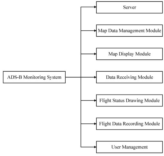
Figure 1.
The basic framework of an ADS-B surveillance system.
2.2. Ionospheric Computerized Tomography
Tomography is essentially the integration of rays passing through an object. Computerized tomography (CT) uses various rays such as electromagnetic waves, radiation, etc., to scan the inside of the detected object from the outside of the detected object. The integral action of the target on the ray determines the internal state of the object. When the ray passes through the interior of the target, it is affected by various factors due to the internal structure of the target, so when the ray comes out, it carries relevant information inside the target. This is the simple working process of tomography technology. Through a suitable reconstruction method, the internal information of the detected target is solved according to the projection data.
The ionospheric tomography process based on simulated ADS-B signal data is roughly as follows: first, the ionospheric tomography area is determined; second, the electronic density grid is divided and the grid electronic density is pixelized; third, according to the TEC data measured by the simulated ADS-B signal data, the projection matrix is determined and a set of equations is established; fourth, the initial value of the algorithm iteration is determined (this article uses the IRI-2012 model as the initial value); finally, a suitable algorithm is chosen to solve the electron density [20,21].
2.2.1. IRI Model
The International Reference Ionospheric Model (IRI) is an international project jointly sponsored by the Space Research Council and the International Radio Science Union. These organizations formed a working group in the late 1960s to produce a standard empirical model of the ionosphere based on all available data sources. Several versions with improved stability have been released. For a given location, date, and time, the IRI model can provide the monthly average electron density, electron temperature, ion temperature, and ion mixture, and the altitude ranges from 50 km to 2000 km. Other parameters provided by the IRI model include the total electron content (TEC), the probability of the extended F generation, the F1 layer area, and the vertical ion drift of the equator [22,23,24].
2.2.2. Multiplicative Algebra Reconstruction
Ionospheric tomography reconstructs the electron density in the inversion area based on the TEC determined by the ADS-B signal data through the ionosphere. The TEC along the satellite signal path can be expressed as
where N(s) is the electron density and l is the propagation path between the satellite and the receiver.
Ionospheric tomographic inversion models are divided into function-based models and pixel-based models. In Equation (1), N(s) changes with time and space. Here, we chose pixel-based models for convenience of inversion. They discretize the inversion space and divide it into several grids, each of which represents a pixel, and the pixel value is the electron density value in the grid. At the same time, it was assumed that within a short period of time, the electron density in the grid remained constant. Then, the TEC on the propagation path of the ADS-B signal can be expressed as the sum of the product of the pixel and the intercept of the ray in the grid:
Equation (2) can be written in a matrix form:
where y is the column vector composed of the TEC obtained from m ADS-B signals; A is the projection matrix composed of the intercept of the ray passing through the pixel area; x is an unknown parameter, that is, the required electron density value, which is an n-dimensional column vector; and e is the discrete error and observation noise. It can be seen from Equation (3) that the tomographic inversion of the pixel-based model is the process of solving x with a known y and A.
In the ionospheric tomographic inversion, due to the limited and uneven number of aircraft and the limitation of the observation elevation angle, a lot of TEC data obtained from the ADS-B signal were missing. An a priori probability model (such as IRI2012) is often added as the initial value of the inversion. This method requires relatively high model accuracy. Due to an insufficient amount of data, some may not be able to mesh rays through ADS-B signals. Thus, the observed data were not corrected.
At present, there are four types of tomographic algorithms that are widely used: Fourier transform, Kalman filter, reconstruction, and model parameter fitting. Line action technology is a widely used method in tomographic theory to solve linear equations which can repeatedly correct the initial value. Each round of iteration is corrected until a satisfactory solution is obtained. Each correction corresponds to one observation, that is, each equation is corrected once. This method saves computer memory and is already in operation, especially involving the calculation of large-scale matrices, and the amount of data is relatively large. These characteristics are particularly important.
This article uses the MART algorithm which is based on the principle of maximum entropy and an a priori model data as the initial value of the ionospheric pixel grid. This paper uses the IRI2012 model as the initial value of the algorithm, and then iteratively corrects it step by step to converge to the optimal solution. Each step of correction corresponds to a TEC, so the amount of observation data had great influence on the accuracy of the result; m steps (m is the number of ADS-B signal rays, that is, the amount of TEC) are iterated into one round. During the iteration process, the electron density is corrected according to the ratio of the integral of the electron density generated by the iteration on the ray and the actually observed oblique TEC, so the result tends to be optimal. The iteration process is as follows:
The initial estimate: , and
The iteration steps:
when and , ,
when and , ;
The equation iteration order is, relaxation factor: , where represents the k + 1 step iteration value for jth pixel and is the inner product.
The MART algorithm converges quickly, generally within 10 rounds of iteration. The biggest advantage of this method is that all solutions are positive, which meets the physical constraint of ionospheric CT inversion on positive electron density. When matrix A is full rank, the algorithm converges to the exact solution of the equations, which are self-consistent and under-timed. If X(0) = e−1l, the algorithm converges to the solution corresponding to the maximum entropy. However, the equations are usually not self-consistent, and the convergence of the algorithm is not very clear. However, the MART algorithm does not fail to converge in the ionospheric CT process [25,26,27,28].
2.2.3. Establishment of Chromatographic Equation
When using the ADS-B signal computer tomography technology to invert the electron density, it is first necessary to define the grid area for the electron density inversion. For the tomographic equation, the TEC can be calculated from the ADS-B signal, and the electron density is required to be solved. It is also necessary to know the intercept of the ray passing through the electron density grid. The ionospheric region, as shown in Figure 2, is divided into eight electron density grids. Assuming that the electron density within the grid changes very little, one pixel can be used to represent the electron density in the grid. A ray passes through the grid area. The ray has intersections with certain sections, and it is cut into several sections by some grids. The lengths of these small sections cut by the grid are the intercepts of the ray in the grid. Let us briefly introduce how to calculate these intercepts.
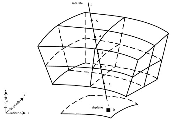
Figure 2.
Principle of ionospheric tomography.
In Figure 2, i is the signal propagation path from airplane to satellite, D and S denote the position of airplane and satellite repectively, the ray intersect the grid interface at five points, denoted by 1, 2, 3, 4 and 5. The intersection points on the height plane are 1, 2, and 5, the longitude plane intersects at Point 4, and the latitude plane intersects at Point 3. Suppose the site coordinates of the aircraft are (, , ) under the WGS-84 coordinates, and the coordinates of the low-orbit satellites are (, , ). Before calculating the intercept of the ray in the grid, the coordinates of the intersection point of the ray and the grid are required. If the coordinates of the aircraft station and the low-orbit satellite are known, the linear equation of the ray can be determined:
Then, the equations of the latitude, longitude, and altitude planes can be determined. The intersection of the straight line and the equation of the corresponding plane is the intersection of the grid that we require.
Latitude surface equation: According to mathematical theory, the latitude surface should be a cone-like surface which can be obtained by rotating a circle around the Z-axis from the connection between a certain point and the center of the Earth. Each point on this surface has the same latitude. If the latitude is Latitude, the latitude surface equation is
Longitude surface equation: The longitude surface should be half of a plane passing through the Z-axis. The angle between the longitude surface and the X-axis is Longitude. The longitude surface equation is
Height surface equation: The height surface is a spherical surface centered on the center of the Earth. The radius of the sphere is the distance from a point on the height surface to the center of the Earth, namely R + Height. The height surface equation is
Simultaneous ray equations and three surface equations can be used to obtain the coordinates of the intersection. According to the coordinates of the intersection, the distance between two adjacent points can be calculated, which is the intercept of the ray passing through the grid area. The distance between point i and point i + 1 is
The intercepts of each grid are obtained in turn, and the coefficient matrix A is arranged in a certain order. Each row of the coefficient matrix represents the intercept of a certain ray in the grid that it passes through. Each column represents the intercept of a different ray in a certain grid, and the intercept of the grid without a ray passing through is zero. In this way, the coefficient matrix is calculated, and the TEC or y was also calculated previously. The problem of calculating the electron density by tomographic inversion becomes the mathematical problem of solving the system of equations and finding matrix x [29,30,31].
3. Results and Discussion
This section selects two areas with a latitude range of 60–70° N/55–85° N and a longitude range of 100–120° E/0–20° E at 0:00 UT on 1 January 2015 as examples to demonstrate the feasibility and effectiveness of the computerized tomography on the ADS-B signal. First, the results in the area within the latitude range of 60–70° N and the longitude range of 100–120° E are shown. Setting the number of airplanes to 18 (approximately distributed in height of 10 km) enables the low-orbit satellites (at height of 1000 km) to receive the ADS-B signal transmitted by airplane. When the inversion of the regional ionospheric electron density occurs, initialization is required. Figure 3 shows the distribution of electron concentration in the inversion area calculated by IRI at 00:00 UTC on 1 January 2015.
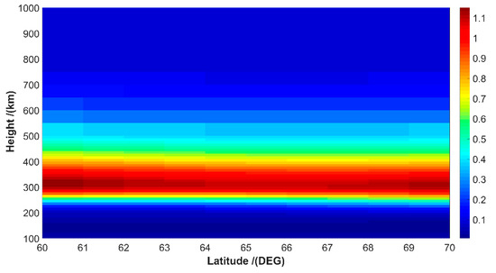
Figure 3.
The distribution of the electron density in the inversion area (60–70° N, 100–120° E) calculated by IRI at 00:00 UTC on 1 January 2015. The unit of electron density is .
Figure 4 shows the electron density along the latitude line in the inversion area at 0:00 UT. It can be seen that for different sections, there was a high-electron-density area between 200 and 300 km and the peak electron density is highly concentrated at 350 km. This result is the same as that of Andrzej Krankowski’s observations of electron density in the ionosphere via FORMOSAT-3/COSMIC and Wen Debao’s result via GPS observations [32,33]. The electron density in this area shows a downward trend as the latitude increases. In the same section, areas with high longitudes in the China region show higher electron density. Huijun Le constructed a two-dimensional map of electron density at different latitudes and longitudes at a 100–700 km altitude around the world by the Grid Modeling Method [34]. The variation trend of electron density in this paper is consistent with his results. The inversion results in Figure 4 are also consistent with those obtained by IGS. The inversion result in Figure 4 was the local morning time in the selected area, and solar radiation was stronger in areas of high longitude and low latitude. This result is consistent with Jiaqi Zhao’s result via compressed sensing (CS) for ionospheric tomography [35].
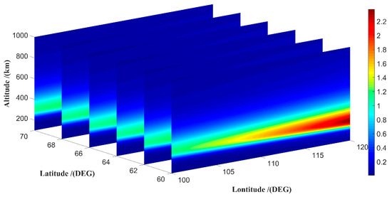
Figure 4.
The electron density along the latitude in the inversion area (60–70° N, 100–120° E) at 0:00 UT. The unit of electron density is
Figure 5 shows the electron density along the meridian of the inversion area at 0:00 UT. Similar to Figure 4, 200–400 km is the height of the high electron density of all slices. The electron density at this height decreased with increasing latitude and increased with increasing longitude. In addition, Figure 6 shows the electron density in the inversion area at different heights at 00:00 UTC. Moreover, it can be seen that the maximum electron density on the tangent plane occurs at a height of 300 km with an approximately 60° latitude and 120° longitude, which is consistent with Figure 4 and Figure 5.
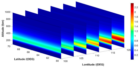
Figure 5.
The electron density along the longitude in the inversion area (60–70° N, 100–120° E) at 0:00 UT. The unit of electron density is
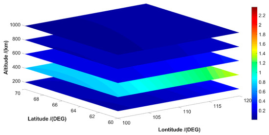
Figure 6.
The electron density along the height in the inversion area (60–70° N, 100–120° E) at 0:00 UT. The unit of the electron density is
In addition, we selected the area with a latitude range of 55–85° N and a longitude range of 0–20° E as the inversion area. Setting the number of airplanes to 18 (approximately distributed to a height of 10 km), low-orbit satellites (at a height of 1000 km) received the ADS-B signal transmitted by the airplane. Figure 7 shows the distribution of the electron concentration in the inversion area calculated by IRI at 00:00 UTC on 1 January 2015.
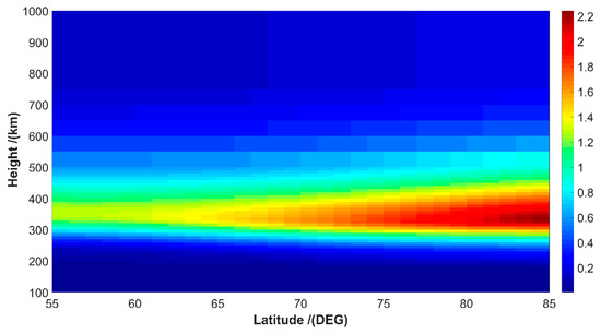
Figure 7.
The distribution of electron concentration in the inversion area calculated by IRI at 00:00 UTC on 1 January 2015. The unit of electron density is
Figure 8 shows the result of the electron density along the latitude in the inversion area at 0:00 UT. It can be seen that there was a high-electron-density area between 200 and 400 km, and the electron density in this area had an upward trend as the latitude increased for different sections. At this time, it was night time in the area, and solar radiation was stronger in the low-longitude and high-latitude areas.
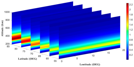
Figure 8.
The electron density along the latitude in the inversion area (55–85° N, 0–20° E) at 0:00 UT. The unit of electron density is
Figure 9 shows the results of the electron density along the meridian in the inversion area at 0:00 UT. Similar to Figure 9, 200–400 km was the highest electron density height of all sections. The electron density at this height increased as the latitude increased, and decreased as the longitude increased. Figure 10 displays the results of the sections of the electron density along the height in the inversion area at 0:00 UT. Moreover, it can be seen that the maximum electron density at a height of 400 km appeared at a latitude of about 85° and a longitude of 0°, which is consistent with Figure 8 and Figure 9.
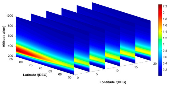
Figure 9.
The electron density along the longitude in the inversion area (55–85° N, 0–20° E) at 0:00 UT. The unit of electron density is
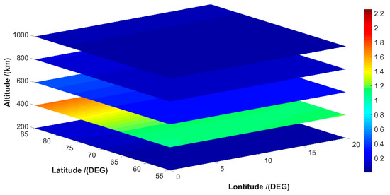
Figure 10.
The electron density along the height in the inversion area (55–85° N, 0–20° E) at 0:00 UT. The unit of electron density is
4. Conclusions
The ADS-B system combines the traditional monitoring system and the communication system into one, and it can be used to carry out ionospheric tomography. To examine the feasibility and effectiveness of computerized tomography on the ADS-B signal, this paper used the IRI-2012 model as the initial value and ionospheric computer tomography technology as the iterative algorithm. Inversion technology from the simulated satellite-borne ADS-B signal data to the regional ionospheric electron density was realized. In addition, the ionospheric electron density values in two different regions (60–70° N, 100–120° E/55–85° N, 0–20° E) at 0:00 UT on 1 January 2015 were selected as examples based on a height resolution of 200 km, latitude resolution of 2°, and longitude resolution of 5°. The results include the inverted ionospheric electron density values along the latitude, longitude, and height, respectively. Compared with the actual situation of ionospheric electron density [32,33,34,35], we found that this inversion method can obtain the electron density effectively, which is of great significance to the study of the ionosphere on a global scale.
Author Contributions
Conceptualization, X.D., Z.Y. and Q.Z.; methodology, H.W. and Y.L.; resources, X.D.; visualization, C.Z., J.Z. and F.S.; funding acquisition, X.D. All authors have read and agreed to the published version of the manuscript.
Funding
This work was supported by the National Natural Science Foundation of China (NSFC grant No. 42176185).
Institutional Review Board Statement
Not applicable.
Informed Consent Statement
Not applicable.
Data Availability Statement
Not applicable.
Acknowledgments
The authors gratefully thank the anonymous reviewers for their insight and help.
Conflicts of Interest
The authors declare no conflict of interest.
References
- Pryse, S.E. Radio Tomography: A New Experimental Technique. Surv. Geophys. 2003, 24, 1–38. [Google Scholar] [CrossRef]
- Aarons, J. Global Morphology of Ionospheric Scintillations. Proc. IEEE 1982, 70, 360–378. [Google Scholar] [CrossRef]
- Alexander, P.; de la Torre, A.; Hierro, R.; Llamedo, P. Assessment of precision in ionospheric electron density profiles retrieved by GPS radio occultations. Adv. Space Res. 2014, 54, 2249–2258. [Google Scholar] [CrossRef]
- Huang, L.; Wang, J.; Jiang, Y.; Huang, J.; Chen, Z.; Zhao, K. A preliminary study of the single crest phenomenon in total electron content (TEC) in the equatorial anomaly region around 120°E longitude between 1999 and 2012. Adv. Space Res. 2014, 54, 2200–2207. [Google Scholar] [CrossRef]
- Brunini, C.; Azpilicueta, F.J. Accuracy assessment of the GPS-based slant total electron content. J. Geodesy 2009, 83, 773–785. [Google Scholar] [CrossRef]
- Sayyed, M.I.; Akman, F.; Geçibesler, I.H.; Tekin, H.O. Measurement of mass attenuation coefficients, effective atomic numbers, and electron densities for different parts of medicinal aromatic plants in low-energy region. Nucl. Sci. Tech. 2018, 29, 144. [Google Scholar] [CrossRef]
- Brandi, F.; Gizzi, L.A. Optical diagnostics for density measurement in high-quality laser-plasma electron accelerators. High Power Laser Sci. Eng. 2019, 7, 40–50. [Google Scholar] [CrossRef]
- Inada, Y.; Aono, K.; Ono, R.; Kumada, A.; Hidaka, K.; Maeyama, M. Two-dimensional electron density measurement of pulsed positive primary streamer discharge in atmospheric-pressure air. J. Phys. D Appl. Phys. 2017, 50, 174005. [Google Scholar] [CrossRef]
- Van Der Pryt, R.; Vincent, R. A Simulation of Reflected ADS-B Signals over the North Atlantic for a Spaceborne Receiver. Positioning 2016, 07, 51–62. [Google Scholar] [CrossRef]
- Cushley, A. Ionospheric Tomography Using Faraday Rotation of Automatic Dependent Surveillance Broadcast (UHF) Signals. Master’s Thesis, Royal Military College of Canada, Kingston, ON, USA, 2013. [Google Scholar]
- Cushley, A.C.; Noël, J.-M. Ionospheric tomography using ADS-B signals. Radio Sci. 2014, 49, 549–563. [Google Scholar] [CrossRef]
- Cushley, A.C.; Kabin, K.; Noël, J.-M. Faraday rotation of Automatic Dependent Surveillance-Broadcst (ADS-B) signals as a method of ionospheric characterization. Radio Sci. 2017, 52, 1293–1300. [Google Scholar] [CrossRef]
- Cushley, A.C.; Noel, J.-M. Ionospheric sounding and tomography using Automatic Identification System (AIS) and other signals of opportunity. Radio Sci. 2020, 55, e2019RS006872. [Google Scholar] [CrossRef]
- Wright, J.W. Ionogram inversion for a tilted ionosphere. Radio Sci. 1990, 25, 1175–1182. [Google Scholar] [CrossRef]
- Liu, Z.; Gao, Y.; Skone, S. A study of smoothed TEC precision inferred from GPS measurements. Earth Planets Space 2005, 57, 999–1007. [Google Scholar] [CrossRef]
- Abdulaziz, A.; Yaro, A.S.; Adam, A.A.; Kabir, M.T.; Salau, H.B. Optimum Receiver for Decoding Automatic Dependent Surveillance Broadcast (ADS-B) Signals. Am. J. Signal Process. 2015, 5, 23–31. [Google Scholar] [CrossRef]
- Zeitlin, A.D.; Strain, R.C. Augmenting ADS-B with Traffic Information Service-Broadcast. IEEE Aerosp. Electron. Syst. Mag. 2003, 18, 13–18. [Google Scholar] [CrossRef]
- Zhang, Z. Optimization Performance Analysis of 1090ES ADS-B Signal Separation Algorithm based on PCA and ICA. Int. J. Perform. Eng. 2018, 14, 741–750. [Google Scholar] [CrossRef]
- Francis, R.; Vincent, R.; Noël, J.; Tremblay, P.; Desjardins, D.; Cushley, A.; Wallace, M. The Flying Laboratory for the Observation of ADS-B Signals. Int. J. Navig. Obs. 2011, 2011, 973656. [Google Scholar] [CrossRef]
- Xu, J.S.; Zou, Y.H.; Ma, S.Y. Time-dependent 3-D Computerized Ionospheric Tomography with Ground-Based GPS Network and Occultation Observations. Chin. J. Geophys. 2005, 48, 835–844. [Google Scholar] [CrossRef]
- Zhou, C.; Lei, Y.; Li, B.; An, J.; Zhu, P.; Jiang, C.; Zhao, Z.; Zhang, Y.; Ni, B.; Wang, Z.; et al. Comparisons of ionospheric electron density distributions reconstructed by GPS computerized tomography, backscatter ionograms, and vertical ionograms. J. Geophys. Res. Space Phys. 2015, 120, 11–32, 47. [Google Scholar] [CrossRef]
- Bilitza, D.; Brown, S.A.; Wang, M.Y.; Souza, J.R.; Roddy, P.A. Measurements and IRI model predictions during the recent solar minimum. J. Atmos. Sol.-Terr. Phy. 2012, 86, 99–106. [Google Scholar] [CrossRef]
- Adeniyi, J.O. Experimental equatorial ionospheric profiles and IRI model profiles. J. Atmos. Sol.-Terr. Phys. 1997, 59, 1205–1208. [Google Scholar] [CrossRef]
- Kimura, I.; Tsunehara, K.; Hikuma, A.; Su, Y.Z.; Kasahara, Y.; Oya, H. Global electron density distribution in the plasmasphere deduced from Akebono wave data and the IRI model. J. Atmos. Sol.-Terr. Phy. 1997, 59, 1569–1586. [Google Scholar] [CrossRef]
- Wen, D.; Wang, Y.; Norman, R. A new two-step algorithm for ionospheric tomography solution. Gps Solut. 2012, 16, 89–94. [Google Scholar] [CrossRef]
- Wen, D.; Liu, S. A new ionospheric tomographic algorithm—Constrained multiplicative algebraic reconstruction technique (CMART). J. Earth Syst. Sci. 2010, 119, 489–496. [Google Scholar] [CrossRef]
- Fougere, P.F. Ionospheric radio tomography using maximum entropy 1. Theory and simulation studies. Radio Sci. 1995, 30, 429–444. [Google Scholar] [CrossRef]
- Buresova, D.; Nava, B.; Galkin, I.; Angling, M.; Stankov, S.M.; Coisson, P. Data ingestion and assimilation in ionospheric models. Ann. Geophys. 2009, 52, 235–253. [Google Scholar] [CrossRef]
- Das, S.K.; Shukla, A.K. Two-dimensional ionospheric tomography over the low-latitude Indian region: An intercomparison of ART and MART algorithms. Radio Sci. 2011, 46, 1–13. [Google Scholar] [CrossRef]
- Wen, D.; Liu, S.; Tang, P. Tomographic reconstruction of ionospheric electron density based on constrained algebraic reconstruction technique. Gps Solut. 2010, 14, 375–380. [Google Scholar] [CrossRef]
- Gritti, F.; Guiochon, G. Fundamental chromatographic equations designed for columns packed with very fine particles and operated at very high pressures. J. Chromatogr. A 2008, 1206, 113–122. [Google Scholar] [CrossRef] [PubMed]
- Krankowski, A.; Zakharenkova, I.; Krypiak-Gregorczyk, A.; Shagimuratov, I.I.; Wielgosz, P. Ionospheric electron density observed by FORMOSAT-3/COSMIC over the European region and validated by ionosonde data. J. Geod. 2011, 85, 949–964. [Google Scholar] [CrossRef]
- Wen, D.; Yuan, Y.; Ou, J. Monitoring the three-dimensional ionospheric electron density distribution using GPS observations over China. J. Earth Syst. Sci. 2007, 116, 235–244. [Google Scholar] [CrossRef]
- Le, H.; Han, T.; Li, Q.; Liu, L.; Chen, Y.; Zhang, H. A new global ionospheric electron density model based on grid modeling method. Space Weather 2022, 20, e2021SW002992. [Google Scholar] [CrossRef]
- Zhao, J.; Tang, Q.; Zhou, C.; Zhao, Z.; Wei, F. Three-dimensional ionospheric tomography based on compressed sensing. GPS Solut. 2023, 27, 90. [Google Scholar] [CrossRef]


Disclaimer/Publisher’s Note: The statements, opinions and data contained in all publications are solely those of the individual author(s) and contributor(s) and not of MDPI and/or the editor(s). MDPI and/or the editor(s) disclaim responsibility for any injury to people or property resulting from any ideas, methods, instructions or products referred to in the content. |
© 2023 by the authors. Licensee MDPI, Basel, Switzerland. This article is an open access article distributed under the terms and conditions of the Creative Commons Attribution (CC BY) license (https://creativecommons.org/licenses/by/4.0/).