Mechanism of the Record-Breaking Heatwave Event Dynamics in South America in January 2022

Abstract

Heatwaves in the Southern Hemisphere (SH) occur frequently but have received little attention over the years. This study presents a comprehensive analysis of a long-duration, wide-ranging, and high-intensity heatwave event in South America spanning from 9 to 16 January 2022. Before the heatwave occurred, the meridional sea surface temperature (SST) in the SH intensified due to the warming of the South Pacific, while the Southern Annular Mode (SAM) exhibited a positive phase. As a result, the intensified wave activities in the westerlies led to high-pressure anomalies in South America, which played a dominant role in the generation of the heatwave. The diagnostic analysis of thermodynamic equations in South America indicates that the temperature increase during the heatwave was primarily caused by the vertical advection term. In contrast, horizontal advection had a negative impact on surface warming. Additionally, the diabatic heating term associated with surface land types serves as a significant factor that cannot be disregarded. This study aims to deepen our understanding of the mechanisms underlying heatwave generation in South America, enabling the improved prediction of heatwaves and enhanced assessment of potential risks in the future.

1. Introduction

In the context of global warming, extreme weather events, including heatwave, drought, and flood, have become increasingly frequent and widespread worldwide [1]. The attribution of these extreme climate events is a complex and crucial task for understanding their causes and impacts [2]. Heatwaves can pose significant risks to people’s lives and property safety [3]. From 2020 to 2022, three consecutive La Niña events were recorded [4]. A La Niña event typically induces cooling effects on North and South America [5,6,7]. However, it is noteworthy that an increased occurrence of heatwaves during La Niña events has been observed in various regions. For instance, notable heatwaves occurred in western North America in 2021, South America in early 2022, and Europe in July 2022, resulting in significant impacts, including forest fires [8].

Numerous studies have been conducted on heatwaves, but a consensus on the exact causes of heatwave events has yet to be reached due to their complex and diverse nature. For instance, a large-scale heatwave occurred in Europe during 2003 and Russia during 2010 [3,9,10,11,12,13,14]. The European heat wave in 2003 resulted in large-scale population deaths in France and significantly reduced crop yields [15]. Trigo et al. [3] suggested that the atmospheric circulation anomalies caused by blocking events play a significant role in the direct impact of the European heatwave in 2003, resulting in a downward motion and subsequent adiabatic temperature increase. Moreover, Folland et al. [16] indicated that changes in the North Atlantic storm track position during summer can influence temperatures in northern Europe, thus making them connected with this heatwave event. Recently, researchers have increasingly highlighted the impact of feedback processes from the surface process on heatwaves. The surface type, such as land surface and vegetation, can significantly influence soil moisture, leading to the persistence of surface temperature during heatwave events [17,18,19,20,21,22,23]. Schumacher et al. [24], through the study of the Russian heatwave in 2010, showed the effects of temperature advection and convection on the local temperature. Dong et al. [25] emphasized the significance of the urban heat island effect in heatwave events. Additionally, marine heatwaves and corresponding teleconnection have gained attention in the SH [26,27,28]. Tropical excited wave trains propagating to South America could lead to heatwave events. Rodrigues et al. [29] suggested that the 2013/2014 marine heatwave in South America was linked to the Rossby wave train propagation resulting from the rapid warming of the Indian Ocean. Chen et al. [30] emphasized the role of sea surface temperature (SST) in marine heatwaves. In general, temperature advection, adiabatic heating in high-pressure conditions, and diabatic heating are all important factors affecting heatwaves. However, when studying heatwave events, the dominating factors vary spatially and temporarily [31]. Consequently, it is crucial to consider the comprehensive effects of various contributing factors.

Compared with the Northern Hemisphere (NH), heatwaves in the Southern Hemisphere (SH), particularly in South America, have received limited attention, despite their frequent occurrence. Feron et al. [32] and Geirinhas et al. [33] indicated that there is an increasing frequency of heatwaves in South America against the background of global warming. In fact, due to the difference in land–sea distribution and topography between the NH and SH, the heatwave mechanism in the SH may be different from that of the NH. Although there have been some studies on heatwaves in South America, there is a lack of comprehensive studies, especially from the perspective of the diabatic heating process caused by the land surface process [34,35,36]. In January 2022, Argentina, Uruguay, and Brazil experienced widespread heatwave characterized by record-breaking high temperatures, with maximum temperatures approaching 45 °C. These extreme weather events significantly impacted the daily electricity consumption of approximately 700,000 users and severely affected the lives of residents in the affected regions [8]. The study and understanding of heatwaves are of utmost importance to better prepare for and mitigate the impacts of such extreme weather events on communities and critical infrastructure.

Motivated by the existing gaps in the multi-angle analysis of heatwave events in the SH, this study is primarily driven by the aim to conduct a comprehensive investigation of the heatwave mechanism in South America. Specifically, the study focuses on a heatwave event that occurred in South America from 9 to 16 January 2022. The subsequent sections of this paper are organized as follows: Section 2 provides an overview of the data and methods employed in this study, while Section 3 presents the key findings derived from the analysis. Finally, Section 4 offers the conclusions and discussion derived from the study.

2. Materials and Methods

2.1. Materials

The data used in this study derive from the ERA5 reanalysis data of the European Center for Medium-Range Weather Forecasts [37]. ERA5 data are of a high quality in terms of climate change [38]. Daily 6h resolution 1° × 1° data are used. This study used air temperature at 12:00 UTC as a proxy of the maximum temperature of the day according to previous studies [23]. Variable daily averages were calculated as the average of the data at 00:00, 06:00, 12:00, and 18:00 UTC. The physical variables involved include near-surface temperature (2 m temperature), surface sensible heat flux, surface latent heat flux, soil moisture (0–7 cm), land cover types, mean sea level pressure, 850 hPa temperature and wind field (u v), 850 hPa diabatic heating data (including mean temperature tendency due to short-wave radiation and mean temperature tendency due to long-wave radiation), 700 hPa vertical velocity, 500 hPa geopotential height, 250 hPa geopotential height, and wind field (u v).

2.2. Methods

The definition of heatwaves can vary dependent on the criteria used. Two approaches are typically employed. The first approach is to adopt the standard of the World Meteorological Organization, where heatwaves are defined as a period during which the daily maximum temperature exceeds the climatological mean specified in the past 30 years by at least 5 K for a minimum of five consecutive days. The second approach is based on positive deviations from the 95% quantile of the climatological maximum temperature distribution [39,40]. This study adopts the latter method for identification and classification. In order to remove the influence of seasonal cycle, in the following analysis, the January from 1979 to 2019 is used as the climatology, and the anomaly is calculated based on this standard. According to the 95% quantile threshold, a prolonged and intensely severe heatwave event occurring from 9 to 16 January 2022 has been identified in South America. This event notably impacted the regions of northeast Argentina, Uruguay, Paraguay, and southern Brazil. The heatwave first began to develop in Argentina and then gradually moved northeastward to southern Paraguay and northwestern Uruguay. As depicted in Figure 1, the area where the heatwave occurred is delineated by a black box, encompassing the region from 25° S to 38° S latitude and 67° W to 52° W longitude.

TN flux [41], also known as the wave activity flux, is used to analyze the wave energy propagation in this study. The TN flux is widely used in the analysis of eddy–mean flow interaction since it well represents the Rossby wave propagation direction as well as energy exchange between eddy and mean flow. The calculation of horizontal wave activity flux is depicted in Equation (1):

$$\overrightarrow{W_h}=\frac{Pcos\phi }{2\left|\overrightarrow{U_c}\right|}\left(\begin{array}{c}\frac{U_c}{a^2{cos}^2\phi }\left[{\left(\frac{\partial {\psi }^{\prime }}{\partial \lambda }\right)}^2-{\psi }^{\prime }\frac{{\partial }^2{\psi }^{\prime }}{\partial {\lambda }^2}\right]+\frac{V_c}{a^{2}cos\phi }\left[\frac{\partial {\psi }^{\prime }}{\partial \lambda }\frac{\partial {\psi }^{\prime }}{\partial \phi }-{\psi }^{\prime }\frac{{\partial }^2{\psi }^{\prime }}{\partial \lambda \partial \phi }\right]\\ \frac{U_c}{a^{2}cos\phi }\left[\frac{\partial {\psi }^{\prime }}{\partial \lambda }\frac{\partial {\psi }^{\prime }}{\partial \phi }-{\psi }^{\prime }\frac{{\partial }^2{\psi }^{\prime }}{\partial \lambda \partial \phi }\right]+\frac{V_c}{a^2}\left[{\left(\frac{\partial {\psi }^{\prime }}{\partial \phi }\right)}^2-{\psi }^{\prime }\frac{{\partial }^2{\psi }^{\prime }}{\partial {\phi }^2}\right]\end{array}\right)$$

(1)

where U_c, V_c, φ, λ, Φ, f, and a represent the climate mean of horizontal wind, latitude, longitude, geopotential, Coriolis parameter, and earth radius, respectively. ${\psi }^{\prime }=\frac{{\Phi }^{\prime }}{f}$ is the perturbation of the quasi-geostrophic stream function relative to the climate field.

The attribution of local temperature increase during the heatwave is based on the thermodynamic energy equation [42]. On the left side of the equation, it represents the local temperature variation, while the three terms on the right side represent the horizontal temperature advection term, the vertical temperature advection term, and the diabatic heating term, respectively. The thermodynamic energy equation takes the form of:

$$\frac{\partial T}{\partial t}=-\stackrel{⃑}{V}·\nabla T+\omega \left(\frac{kT}{p}-\frac{\partial T}{\partial p}\right)+\frac{Q}{C_p}$$

$$Q=Q_{rad}+Q_{non-rad} Q_{rad}=Q_{short}+Q_{long} Q_{non-rad}=Q_{latent}+Q_{mixing}$$

(2)

where$T, \stackrel{⃑}{V}, w, p, \mathrm{and} C_p$represent temperature, horizontal wind field, vertical velocity at pressure coordinate, pressure, and specific heat capacity at constant pressure, respectively. $k$ takes the constant 0.286. The parameter Q represents diabatic heating, which could be further divided into radiative $\left(Q_{rad}\right)$ and non-radiative ${(Q}_{non-rad})$ compoents. The radiative term ${(Q}_{rad})$ stems from short-wave radiation${(Q}_{short})$ and long-wave radiation ${(Q}_{long})$. The non-radiative term ${(Q}_{non-rad})$in Equation (2) encompasses a latent heating term ($Q_{latent}$) attributed to moist physics and a mixing element ($Q_{mixing}$) linked to turbulent mixing. Generally, the mixing term’s magnitude ${(Q}_{mixing})$ is relatively smaller when compared to that of the latent heating term $\left(Q_{latent}\right).$ However, local variations in the mixing term can be as substantial as variations in the radiative term or latent heating term [43].

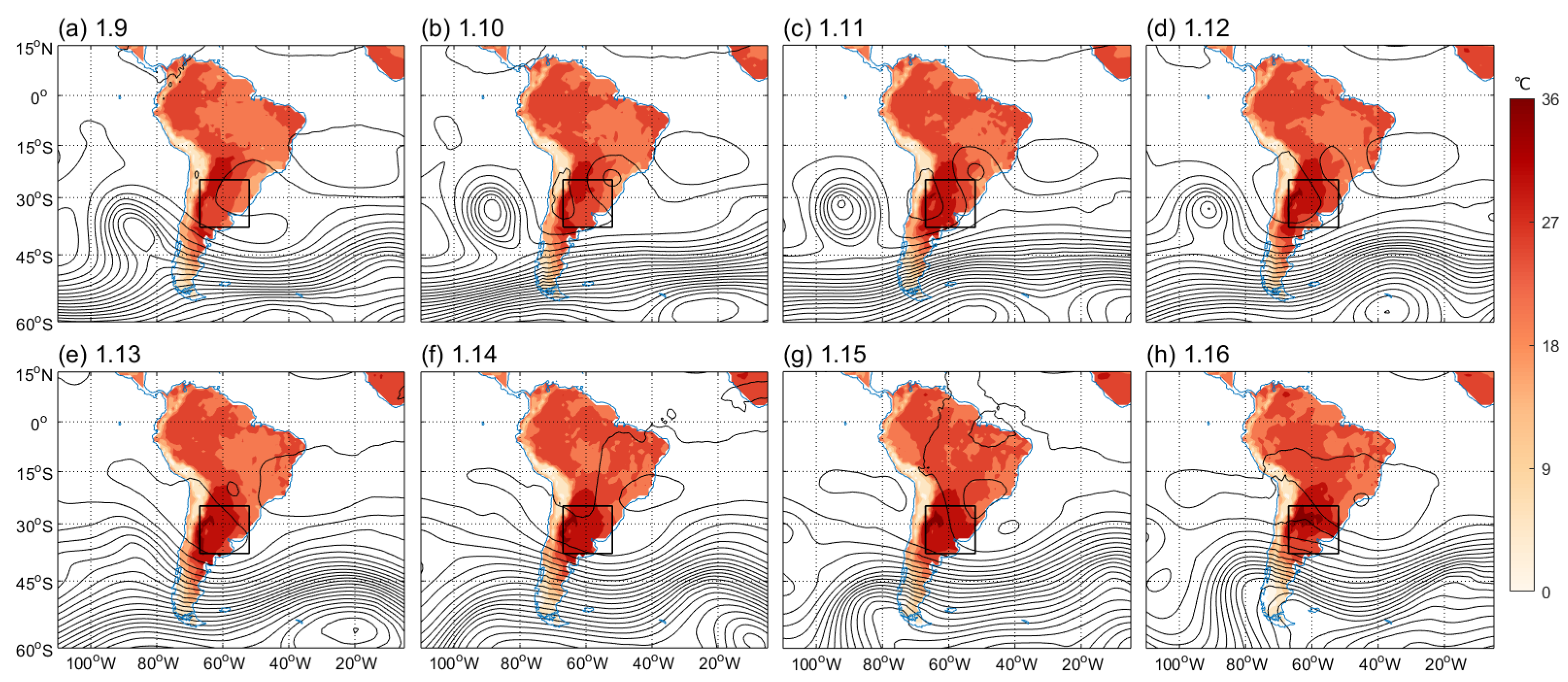
3. Dynamics Analysis of Heatwave in South America on 9 to 16 January

The dominant factors driving heatwave events can vary across different cases [31]. In this section, we commence by presenting the large-scale circulation patterns associated with the heatwave event and further explore its origin from sea surface temperature forcing. Subsequently, our focus shifts to investigating the local processes based on the thermodynamic energy equation. As the heatwave can be primarily locally attributed to three main factors, temperature advection, adiabatic warming resulting from vertical advection, and diabatic heating, we will systematically examine each of these aspects to comprehensively understand the underlying mechanisms in this specific heatwave case.

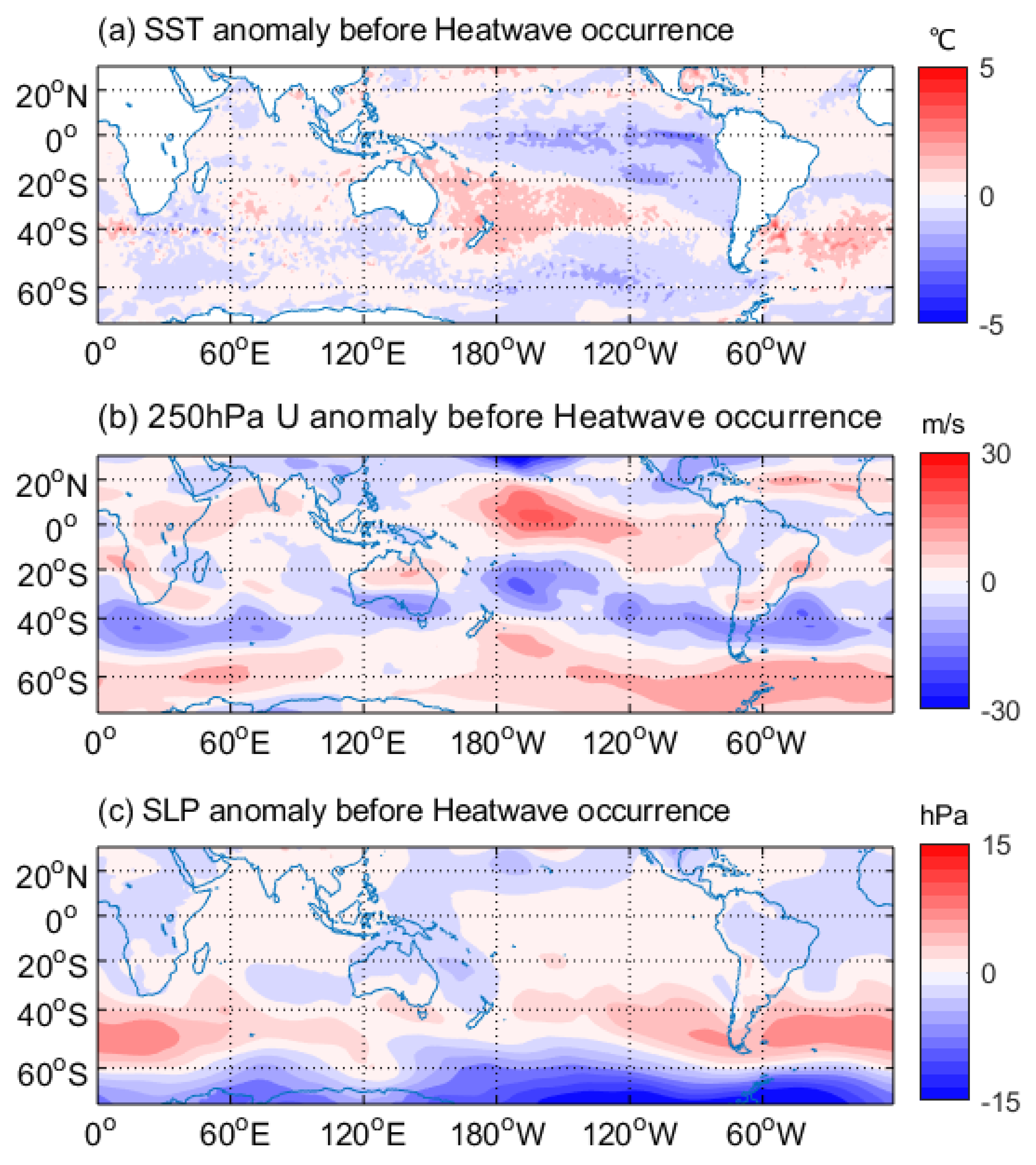
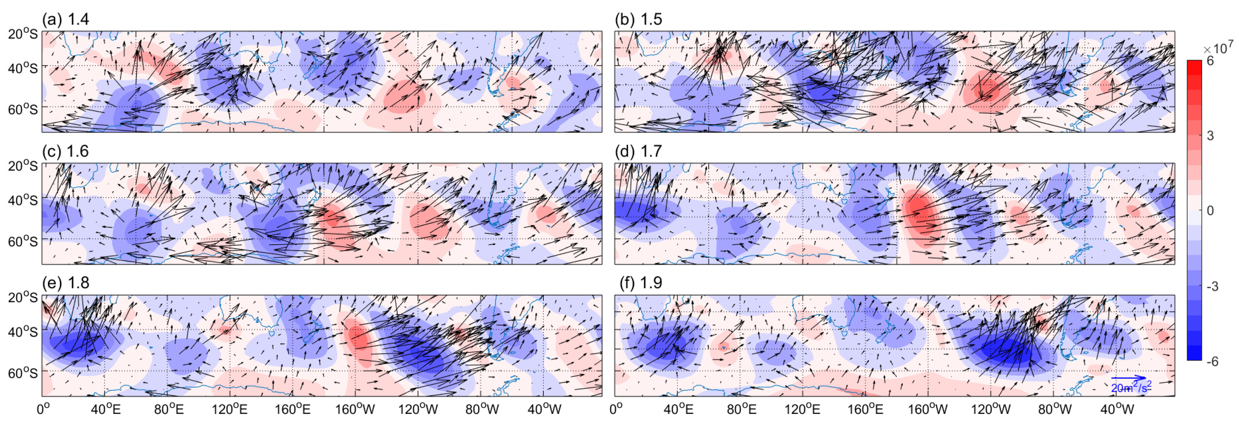
3.1. General Circulation Analysis

Figure 1 illustrates the gradual buildup of high-pressure systems in northern Argentina and Uruguay from 9 to 16 January, which serves as the main cause of the heatwave event. On January 9, the area of interest (depicted by the black box) was situated between a strong ridge to the west and a trough to the east in the westerlies (Figure 1a). From 9 to 13 January, the western ridge gradually transformed into an independent anticyclone and eventually merged with the subtropical high over the South Atlantic on January 14, forming a large anticyclone (Figure 1b–f). This development of the anticyclone coincided with a notable increase in surface temperatures, indicating the occurrence of the heatwave event. From 15 to 16 January, the anticyclone gradually retreated equatorward, marking the end of the heatwave event (Figure 1g,h). The development of the anticyclone from the ridge suggests a potential contribution from wave activities in the westerlies. According to Rodrigues et al. [29], disturbances originating from the tropics, such as the rapid warming of the Indian Ocean, can trigger Rossby waves towards the mid-latitudes in the SH, leading to weather anomalies in South America. This highlights the significant impact of wave trains originating from upstream regions on weather processes in South America.

Figure 2a provides a comprehensive visualization of sea surface temperature (SST) anomalies observed in December 2021. One salient feature is the pronounced presence of positive SST anomalies notably concentrated along the 40°S latitude line, with a distinct emphasis within the South Pacific. This phenomenon induces a significant amplification of the meridional SST gradient. The implications of this thermal gradient are manifested through the thermal wind relation, where it triggers the development of easterly anomalies within the midlatitudes of the upper troposphere and westerly anomalies within the polar region (Figure 2b). Consequently, westerly jet shifts poleward, which leads to more wave generation in the South Pacific due to increased baroclinicity.

Significantly, the sea surface pressure distribution lends further weight to this intricate narrative. Evidently, positive anomalies prevail along the 40° S latitude line, while conversely, negative anomalies dominate along the 65° S line (as illustrated in Figure 2c). This observation strikingly aligns with a distinct phase of the positive Southern Annular Mode (SAM) [44]. Notably, one of the characteristic features of the positive SAM is the poleward shift of the westerly jet.

In a broader synthesis, the anomalous sea surface temperature (SST) patterns in December 2021 emerge as catalysts for alterations in the meridional surface temperature gradient. This gradient perturbation subsequently triggers a pronounced poleward movement of the westerly jet, a hallmark manifestation of the positive SAM.

Figure 3 illustrates the evolution of TN flux over the region with an increased meridional SST gradient in the South Pacific before the occurrence of the heatwave. On January 4 and 5, the wave activities were amplified over the South Pacific (Figure 3a,b). Then, the anomalies propagate eastward to South America, leading to the establishment of a high-pressure system in the region on 6 January (Figure 3c). On 7 and 8 January, the wave train from the South Pacific to South America persisted (Figure 3d,e) and eventually dissipated on 9 January (Figure 3f). It is obvious that the wave train from the South Pacific to South America emerged before the heatwave event. This diagnosis suggests that the eddy activities over the heatwave area are strongly connected with the propagation of an anomalous wave train from South Pacific to South America.

In summary, the above results demonstrate that subtropical ocean warming in December 2021 creates a pronounced meridional temperature gradient, resulting in positive anomalies in the SAM. The positive SAM induces a southward shift in the westerly jet, leading to increased eddy activities. As a result, a wave train propagation from South Pacific to South America came into being and eventually caused the high-pressure system in South America, leading to the 2022 South America heatwave event.

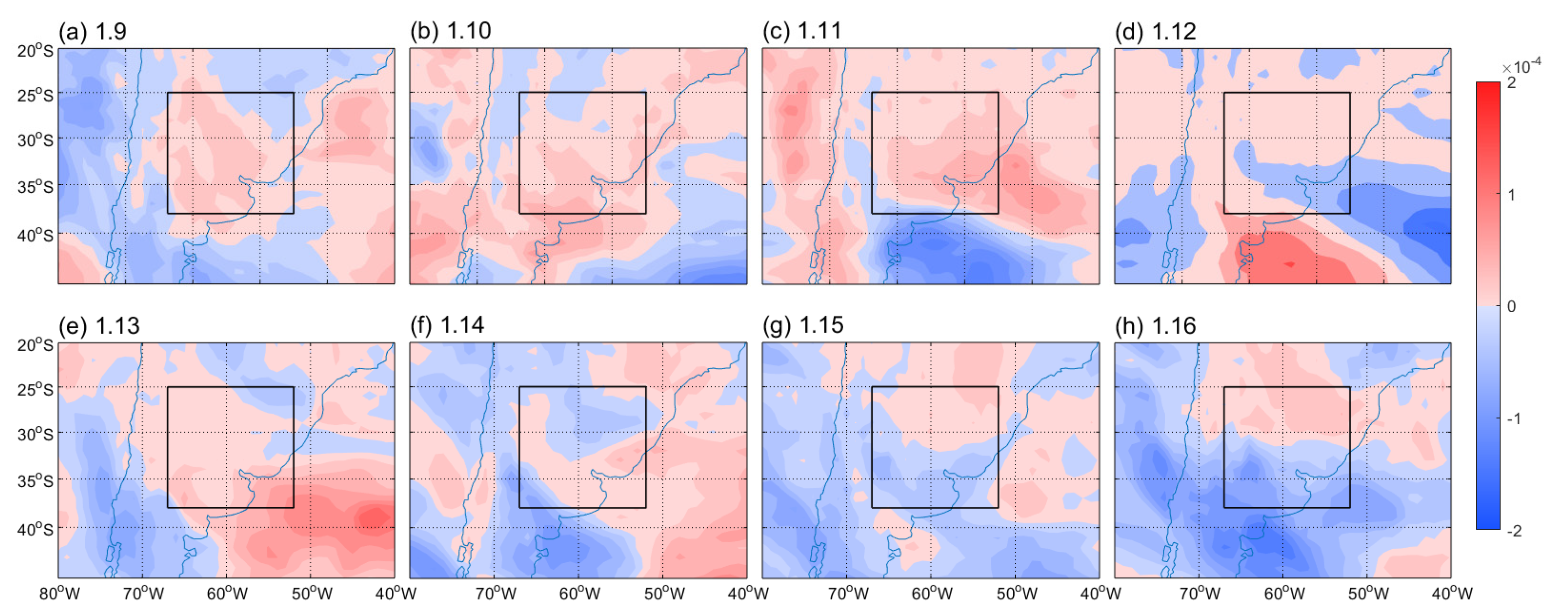
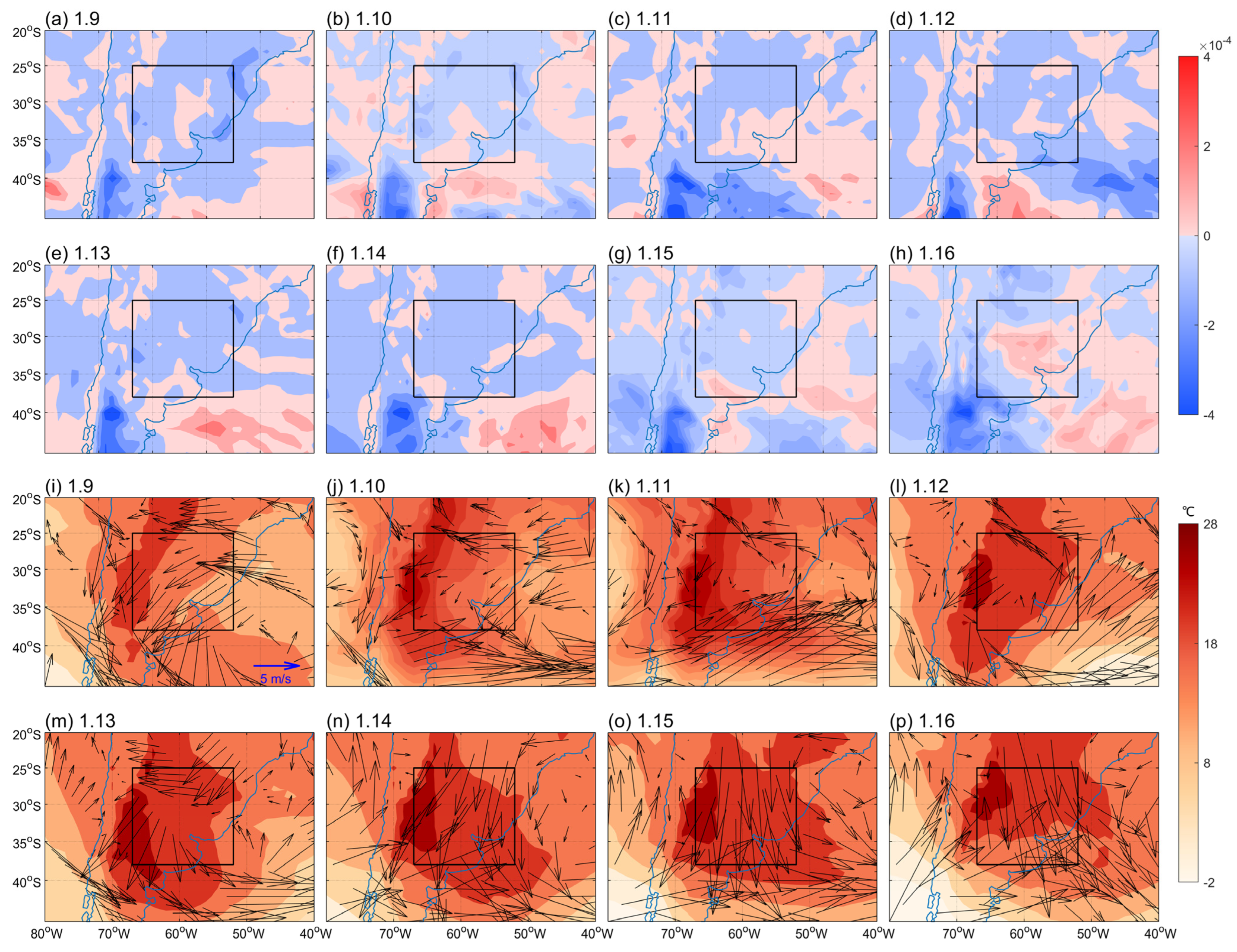
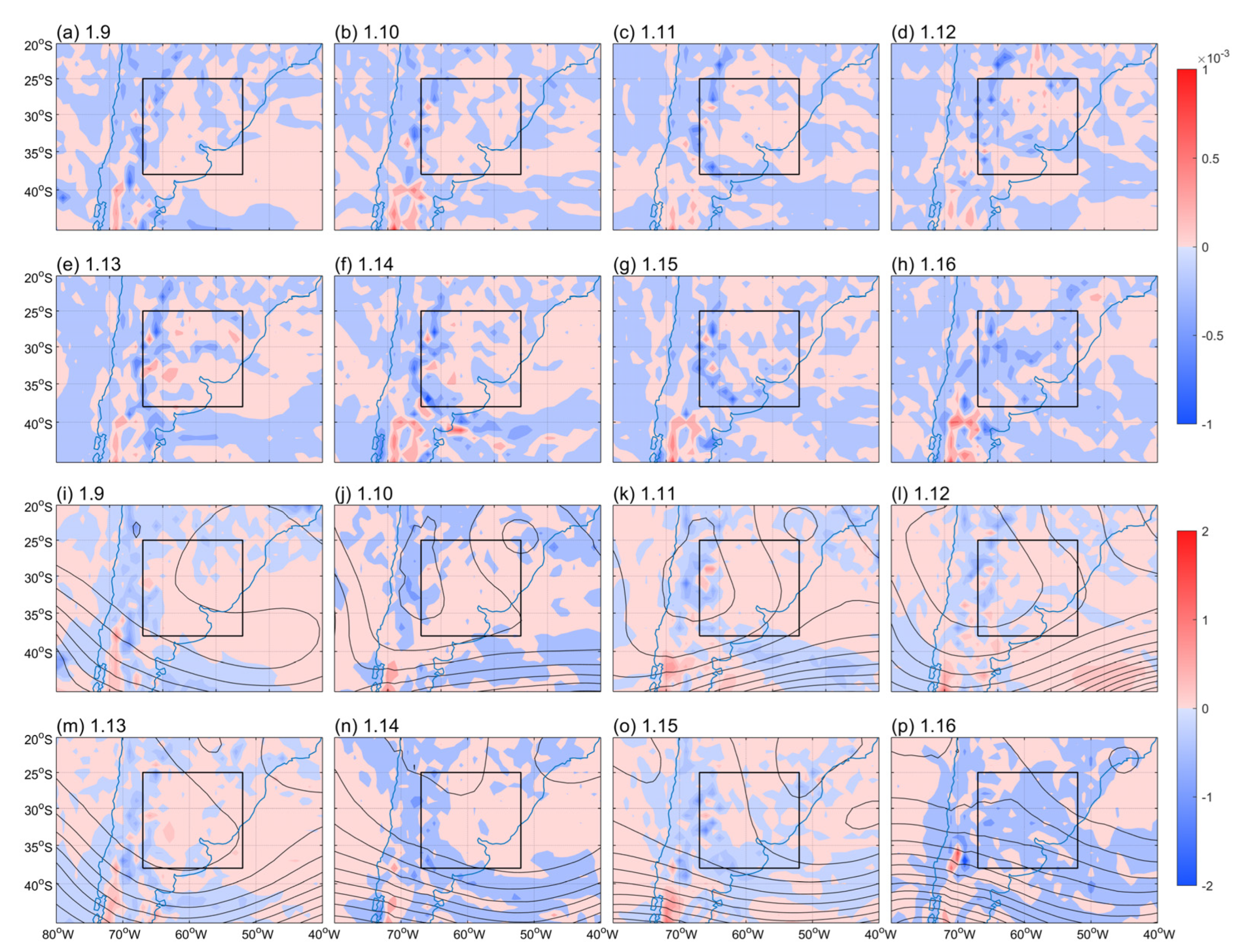
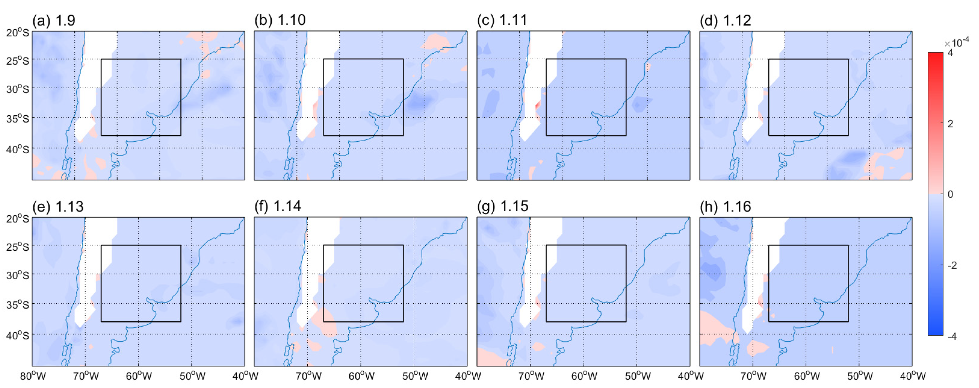
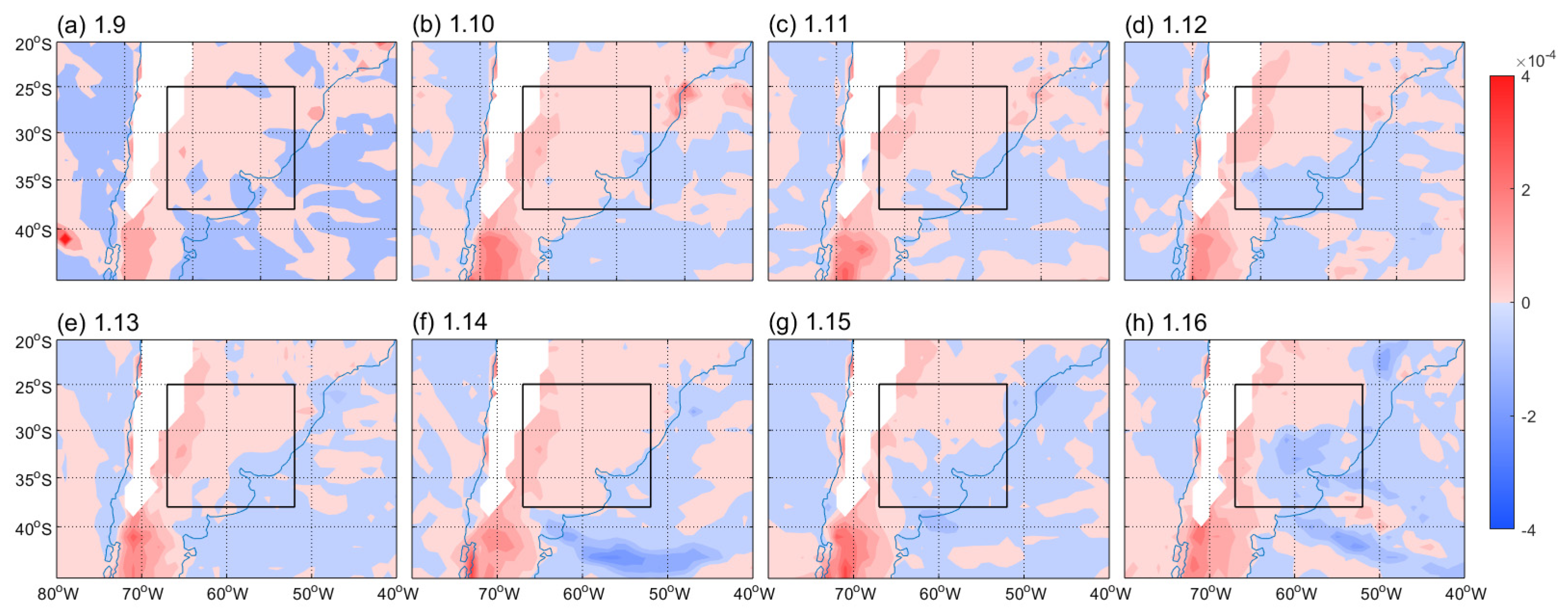
3.2. Local Thermodynamics Analysis

In order to better understand the causes of the heatwave event from a local perspective, a thermodynamic energy equation at 850 hPa is used to diagnose the heatwave event. Figure 4 depicts that the evolution of temperature tendency $\partial$T/$\partial$t throughout the heatwave event. As depicted in Figure 4a–e, in the early stage of this heatwave event, a warming tendency dominates this region, which means the onset of a heatwave and the gradual increase in temperature in this region. Conversely, as shown in the late stage of heatwave (Figure 4f–h), a negative temperature tendency starts to appear and gradually dominates this region, which indicates the end of the heatwave and the gradual decrease in temperature.

Schumacher et al., (2019) suggested that horizontal temperature advection plays an important role in heatwaves. Therefore, we explore the horizontal advection term in the thermodynamic equation at 850 hPa. As Figure 5 shows, unlike most warm advections that favor heatwave occurrences, there is no significant warm horizontal temperature advection in this particular heatwave event. Instead, the cold temperature advection dominates the region (Figure 5a–h). As shown in Figure 5i–o, the overall horizontal wind is northerly and blows out from the area with a relatively high temperature. Consequently, the result shows a cold horizontal temperature advection within the heatwave region.

Next, the contribution of the adiabatic heating from the vertical motion term is examined. From Figure 6a–g, the vertical motion term mainly contributes positively in the heatwave area, which is also consistent with the evolution of the high-pressure system in Figure 1. On 16 January, the last day of the heatwave, as the high-pressure system retreated northwards, the vertical motion weakened, resulting in negative anomalies of vertical motion term (Figure 6h). As shown in Figure 6i–p, in the area where heatwave occurs, the early stage is dominated by the downward movement controlled by high pressure. During the last days of Figure 6o,p, due to weakening of the high-pressure system, the subduction turns into an ascending motion. In general, the contribution of vertical motion to temperature has a good correspondence with the vertical velocity. Overall, the vertical motion term plays a crucial role in the local temperature increase. Taking into account the general circulation analysis in the last section, the high-pressure system in the SH, triggered by the wave train, induces a downward motion, which subsequently results in adiabatic warming. This adiabatic warming emerges as a dominant factor contributing to the local temperature increase during the heatwave event.

Last but not least, diabatic heating is also involved with the heatwave event. As Figure 7 shows, from 9 to 14 January, the diabatic heating term makes a positive contribution over the majority of the heatwave region except for the coastline. During the last two days of the heatwave, diabatic heating had a negative effect on the heatwave region. The variation pattern of the diabatic heating term is similar to that of the vertical motion term, exerting a positive influence on local temperature increases in the early and middle stages of the heatwave and local temperature decrease at the end. Overall, the contribution of the diabatic heating term is not as prominent as that of the vertical motion term, but the effects of this significant factor that cannot be disregarded. Diabatic heating could be divided into multiple terms. Therefore, we further explore the contribution of each term in the diabatic heating term.

As depicted in Figure 8, the net radiation term has a negative impact on the local air temperature increase at 850 hPa during the heatwave period, which is mainly due to the negative effect of longwave radiation caused by high air temperature (not shown). As shown in Figure 6i–p, the prevalence of high pressure during the heatwave period leads to subsidence, which inhibits local convection. Consequently, there is a reduced release of latent heating from condensation caused by convective precipitation. As a result, the mixing term in Equation (2), including surface sensible heat and latent heat, becomes the primary contributor in the non-radiative component of the diabatic heating term (Figure 9). The evolution of the mixing term is similar to that of the diabatic heating term and the vertical term. In the early stage of the heatwave, the positive contribution prevails in the heatwave region, while in the last two days, the negative contribution becomes more prominent. The mixing term is related to land surface processes, such as the surface land types and changes in soil moisture. Figure 10a illustrates that the land cover near the surface is mainly composed of cropland, grassland, and urban human activities. However, during this heatwave event, the near-surface soil moisture was low (Figure 10b), resulting in amplified sensible heating and diminished latent heating near the surface (Figure 10c,d). Meanwhile, increased wind speeds amplify the magnitude of both sensible and latent heat (Figure 5). Consequently, the low-level atmosphere is heated by the increasing sensible heat, further amplifying the effect of the heatwave. The relationship between the mixing term and land use type suggests that human activities have the potential to exacerbate heatwave events.

4. Conclusions and Discussion

This study mainly focuses on the cause and relevant mechanism of a long-duration, high-intensity heatwave event that occurred in northeastern Argentina, Uruguay, Paraguay, and southern Brazil from 9 to 16 January 2022. The analysis reveals that the heatwave event was preceded by anomalous warming of the SST in the South Pacific, leading to an intensified SST gradient and a positive phase of the SAM. As a result, the wave activities became more active and the wave train from the South Pacific propagated to South America, causing high pressure in South America as well as a corresponding heatwave event. By utilizing diagnostic analysis and thermodynamic equations, we demonstrate that the vertical motion term emerged as a dominant contributor to positive temperature changes during the heatwave while the event was characterized by persistent cold horizontal temperature advection. Furthermore, the diabatic heating term, particularly the mixing term, played a significant role in the heatwave. Notably, the surface types in the affected region, predominantly consisting of crops and grasslands, experienced depleted soil moisture, which intensified sensible heating and reduced latent heating. This contributed to the overall diabatic heating and further amplified the impact of the heatwave event. Our study indicates that both internal variability and human activities contribute to the heatwave event, which provides a new perspective to look into the heatwave studies.

In the context of global warming, extreme weather events such as heatwaves become more frequent and their impacts are increasingly significant [1]. Ferron et al. [32] and Geirinhas et al. [33] showed that heatwaves in South America occur frequently with global warming; however, little attention has been paid to heatwaves in South America at present, and its dynamic mechanism has not been fully studied. So, this article hopes to enhance the understanding of the dynamic mechanism of heatwaves in South America through a case study. By deepening our knowledge of heatwave mechanisms and characteristics, we can improve our heatwave prediction capabilities and assess potential risks for the future. This research contributes to the broader scientific understanding of heatwaves and supports efforts to mitigate their adverse effects in a changing climate.

References

1. IPCC. Climate Change 2021: The Physical Science Basis. Contribution of Working Group I to the Sixth Assessment Report of the Intergovernmental Panel on Climate Change; Masson-Delmotte, V., Zhai, P., Pirani, A., Connors, S., Péan, C., Berger, S., Caud, N., Chen, Y., Goldfarb, L., Gomis, M., et al., Eds.; Cambridge University Press: Cambridge, UK; New York, NY, USA, 2021. [Google Scholar]
2. Trenberth, K.E.; Fasullo, J.T.; Shepherd, T.G. Attribution of climate extreme events. Nat. Clim. Chang. 2015, 5, 725–730. [Google Scholar] [CrossRef]
3. Trigo, R.M.; García-Herrera, R.; Díaz, J.; Trigo, I.F.; Valente, M.A. How exceptional was the early August 2003 heatwave in France? Geophys. Res. Lett. 2005, 32, L10701. [Google Scholar] [CrossRef]
4. Shi, L.; Ding, R.; Hu, S.; Li, X.; Li, J. Extratropical impacts on the 2020–2023 Triple-Dip La Niña event. Atmos. Res. 2023, 294, 106937. [Google Scholar] [CrossRef]
5. Kiladis, G.N.; Diaz, H.F. Global climatic anomalies associated with extremes in the Southern Oscillation. J. Clim. 1989, 2, 1069–1090. [Google Scholar] [CrossRef]
6. Barros, V.R.; Grimm, A.M.; Doyle, M.E. Relationship between temperature and circulation in southeastern South America and its influence from El Niño and La Niña events. J. Meteorol. Soc. Jpn. 2002, 80, 21–32. [Google Scholar] [CrossRef]
7. Infanti, J.M.; Kirtman, B.P. North American rainfall and temperature prediction response to the diversity of ENSO. Clim. Dyn. 2015, 46, 3007–3023. [Google Scholar] [CrossRef]
8. Wikipedia. 2022 Heat Waves, Wikipedia, the Free Encyclopedia. 2022. Available online: https://en.wikipedia.org/wiki/2022_heat_waves (accessed on 1 July 2023).
9. Barriopedro, D.; Fischer, E.M.; Luterbacher, J.; Trigo, R.M.; Garcia-Herrera, R. The hot summer of 2010: Redrawing the temperature record map of Europe. Science 2011, 332, 220–224. [Google Scholar] [CrossRef]
10. Fink, A.H.; Brücher, T.; Krüger, A.; Leckebusch, G.C.; Pinto, J.G.; Ulbrich, U. The 2003 European summer heatwaves and drought-synoptic diagnosis and impacts. Weather 2004, 59, 209–216. [Google Scholar] [CrossRef]
11. Fischer, E.M.; Schär, C. Consistent geographical patterns of changes in high-impact European heatwaves. Nat. Geosci. 2010, 3, 398–403. [Google Scholar] [CrossRef]
12. García-Herrera, R.; Díaz, J.; Trigo, R.M.; Luterbacher, J.; Fischer, E.M. A Review of the European Summer Heat Wave of 2003. Crit. Rev. Environ. Sci. Technol. 2010, 40, 267–306. [Google Scholar] [CrossRef]
13. Schär, C.; Vidale, P.L.; Lüthi, D.; Frei, C.; Häberli, C.; Liniger, M.A.; Appenzeller, C. The role of increasing temperature variability in European summer heatwaves. Nature 2004, 427, 332–336. [Google Scholar] [CrossRef] [PubMed]
14. Seneviratne, S.I.; Luthi, D.; Litschi, M.; Schar, C. Land-atmosphere coupling and climate change in Europe. Nature 2006, 443, 205–209. [Google Scholar] [CrossRef] [PubMed]
15. Ciais, P.; Reichstein, M.; Viovy, N.; Granier, A.; Ogée, J.; Allard, V.; Aubinet, M.; Buchmann, N.; Bernhofer, C.; Carrara, A.; et al. Europe-wide reduction in primary productivity caused by the heat and drought in 2003. Nature 2005, 437, 529–533. [Google Scholar] [CrossRef] [PubMed]
16. Folland, C.K.; Knight, J.; Linderholm, H.W.; Fereday, D.; Ineson, S.; Hurrell, J.W. The Summer North Atlantic Oscillation: Past, Present, and Future. J. Clim. 2009, 22, 1082–1103. [Google Scholar] [CrossRef]
17. Berg, A.; Lintner, B.R.; Findell, K.L.; Malyshev, S.; Loikith, P.C.; Gentine, P. Impact of Soil Moisture–Atmosphere Interactions on Surface Temperature Distribution. J. Clim. 2014, 27, 7976–7993. [Google Scholar] [CrossRef]
18. Fischer, E.M.; Seneviratne, S.I.; Lüthi, D.; Schär, C. Contribution of land-atmosphere coupling to recent European summer heat waves. Geophys. Res. Lett. 2007, 34, L06707. [Google Scholar] [CrossRef]
19. Fischer, E.M.; Seneviratne, S.I.; Vidale, P.L.; Lüthi, D.; Schär, C. Soil Moisture–Atmosphere Interactions during the 2003 European Summer Heat Wave. J. Clim. 2007, 20, 5081–5099. [Google Scholar] [CrossRef]
20. Hirsch, A.L.; Pitman, A.J.; Kala, J. The role of land cover change in modulating the soil moisture-temperature land-atmosphere coupling strength over Australia. Geophys. Res. Lett. 2014, 41, 5883–5890. [Google Scholar] [CrossRef]
21. Liu, X.; He, B.; Guo, L.; Huang, L.; Chen, D. Similarities and Differences in the Mechanisms Causing the European Summer Heatwaves in 2003, 2010, and 2018. Earth’s Future 2020, 8, e2019EF001386. [Google Scholar] [CrossRef]
22. Miralles, D.G.; van den Berg, M.J.; Teuling, A.J.; de Jeu RA, M. Soil moisture-temperature coupling: A multiscale observational analysis. Geophys. Res. Lett. 2012, 39, L21707. [Google Scholar] [CrossRef]
23. Miralles, D.G.; Teuling, A.J.; van Heerwaarden, C.C.; Vilà-Guerau de Arellano, J. Mega-heatwave temperatures due to combined soil desiccation and atmospheric heat accumulation. Nat. Geosci. 2014, 7, 345–349. [Google Scholar] [CrossRef]
24. Schumacher, D.L.; Keune, J.; van Heerwaarden, C.C.; Vilà-Guerau de Arellano, J.; Teuling, A.J.; Miralles, D.G. Amplification of mega-heatwaves through heat torrents fuelled by upwind drought. Nat. Geosci. 2019, 12, 712–717. [Google Scholar] [CrossRef]
25. Dong, L.; Mitra, C.; Greer, S.; Burt, E. The Dynamical Linkage of Atmospheric Blocking to Drought, Heatwave and Urban Heat Island in Southeastern US: A Multi-Scale Case Study. Atmosphere 2018, 9, 33. [Google Scholar] [CrossRef]
26. Cook, K.H. A Southern Hemisphere wave response to ENSO with implications for southern Africa precipitation. J. Atmos. Sci. 2001, 58, 2146–2162. [Google Scholar] [CrossRef]
27. Li, X.; Cai, W.; Meehl, G.A.; Chen, D.; Yuan, X.; Raphael, M.; Holland, D.M.; Ding, Q.; Fogt, R.L.; Markle, B.R.; et al. Tropical teleconnection impacts on Antarctic climate changes. Nat. Rev. Earth Environ. 2021, 2, 680–698. [Google Scholar] [CrossRef]
28. Zhang, B.; Dong, L.; Ding, H.; Xie, Z. ENSO-related Southern Hemisphere blocking dynamics. J. Geophys. Res. Atmos. 2023, 128, e2022JD038087. [Google Scholar] [CrossRef]
29. Rodrigues, R.R.; Taschetto, A.S.; Sen Gupta, A.; Foltz, G.R. Common cause for severe droughts in South America and marine heatwaves in the South Atlantic. Nat. Geosci. 2019, 12, 620–626. [Google Scholar] [CrossRef]
30. Chen, R.; Wen, Z.; Lu, R.; Wang, C. Causes of the Extreme Hot Midsummer in Central and South China during 2017: Role of the Western Tropical Pacific Warming. Adv. Atmos. Sci. 2019, 36, 465–478. [Google Scholar] [CrossRef]
31. Röthlisberger, M.; Papritz, L. Quantifying the physical processes leading to atmospheric hot extremes at a global scale. Nat. Geosci. 2023, 16, 210–216. [Google Scholar] [CrossRef]
32. Feron, S.; Cordero, R.R.; Damiani, A.; Llanillo, P.J.; Jorquera, J.; Sepulveda, E.; Asencio, V.; Laroze, D.; Labbe, F.; Carrasco, J.; et al. Observations and Projections of Heat Waves in South America. Sci. Rep. 2019, 9, 8173. [Google Scholar] [CrossRef]
33. Geirinhas, J.L.; Russo, A.; Libonati, R.; Sousa, P.M.; Miralles, D.G.; Trigo, R.M. Recent increasing frequency of compound summer drought and heatwaves in Southeast Brazil. Environ. Res. Lett. 2021, 16, 034036. [Google Scholar] [CrossRef]
34. Geirinhas, J.L.; Trigo, R.M.; Libonati, R.; Coelho, C.A.S.; Palmeira, A.C. Climatic and synoptic characterization of heat waves in Brazil. Int. J. Climatol. 2018, 38, 1760–1776. [Google Scholar] [CrossRef]
35. Marengo, J.A.; Ambrizzi, T.; Barreto, N.; Cunha, A.P.; Ramos, A.M.; Skansi, M.; Carpio, J.M.; Salinas, R. The heat wave of October 2020 in central South America. Int. J. Climatol. 2021, 42, 2281–2298. [Google Scholar] [CrossRef]
36. Jacques-Coper, M.; Veloso-Aguila, D.; Segura, C.; Valencia, A. Intraseasonal teleconnections leading to heat waves in central Chile. Int. J. Climatol. 2021, 41, 4712–4731. [Google Scholar] [CrossRef]
37. Hersbach, H.; Bell, B.; Berrisford, P.; Biavati, G.; Horányi, A.; Muñoz Sabater, J.; Nicolas, J.; Peubey, C.; Radu, R.; Schepers, D.; et al. ERA5 Hourly Data on Pressure Levels from 1959 to Present. Q. J. R. Meteorol. Soc. 2020, 146, 1999–2049. [Google Scholar] [CrossRef]
38. Dole, R.; Hoerling, M.; Perlwitz, J.; Eischeid, J.; Pegion, P.; Zhang, T.; Quan, X.-W.; Xu, T.; Murray, D. Was there a basis for anticipating the 2010 Russian heat wave? Geophys. Res. Lett. 2011, 38, L06702. [Google Scholar] [CrossRef]
39. Lhotka, O.; Kyselý, J. Characterizing joint effects of spatial extent, temperature magnitude and duration of heat waves and cold spells over Central Europe. Int. J. Climatol. 2015, 35, 1232–1244. [Google Scholar] [CrossRef]
40. Russo, S.; Dosio, A.; Graversen, R.G.; Sillmann, J.; Carrao, H.; Dunbar, M.B.; Singleton, A.; Montagna, P.; Barbola, P.; Vogt, J.V. Magnitude of extreme heat waves in present climate and their projection in a warming world. J. Geophys. Res. Atmos. 2014, 119, 12500–12512. [Google Scholar] [CrossRef]
41. Takaya, K.; Nakamura, H. A Formulation of a Phase-Independent Wave-Activity Flux for Stationary and Migratory Quasigeostrophic Eddies on a Zonally Varying Basic Flow. J. Atmos. Sci. 2001, 58, 608–627. [Google Scholar] [CrossRef]
42. Wright, J.S.; Fueglistaler, S. Large differences in reanalyses of diabatic heating in the tropical upper troposphere and lower stratosphere. Atmos. Chem. Phys. 2013, 13, 9565–9576. [Google Scholar] [CrossRef]
43. Flannaghan, T.J.; Fueglistaler, S. Kelvin waves and shear-flow turbulent mixing in the TTL in (re-)analysis data. Geophys. Res. Lett. 2011, 38, L02801. [Google Scholar] [CrossRef]
44. Gong, D.; Wang, S. Definition of Antarctic Oscillation index. Geophys. Res. Lett. 1999, 26, 459–462. [Google Scholar] [CrossRef]
Figure 1. The heatwave that occurred in South America from 9 to 16 January 2022 for (a) 1.9, (b) 1.10, (c) 1.11, (d) 1.12, (e) 1.13, (f) 1.14, (g) 1.15, (h) 1.16. The shaded is the daily average near-surface temperature, in units of °C, and the contour is the geopotential heights at 500 hPa with ranges from 4800 to 6000 gpm and interval as 40 gpm. The area represented by the black box is where a heatwave occurred (The black box in the pictures below represents the same meaning).
Atmosphere 14 01326 g001
Figure 2. In December 2021, (a) the SST anomaly in the SH compared with the same period in the climatology, (b) the 250 hPa zonal wind anomaly in the SH compared with the same period in the climatology, (c) the SLP anomaly in the SH compared with the same period in the climatology.
Atmosphere 14 01326 g002
Figure 3. The horizontal component of TN flux at 250 hPa. The shaded represents perturbation of the stream function, in units of m2/s, and the arrow represents the horizontal component of TN flux, in units of m2/s2. For (a) 1.4, (b) 1.5, (c) 1.6, (d) 1.7, (e) 1.8, (f) 1.9. The blue arrow at the bottom right of (f) represents the quiverkey in units of m2/s2.
Atmosphere 14 01326 g003
Figure 4. The evolution of T/ t (units: °C/s ) in heatwave event from 9 to 16 January for (a) 1.9, (b) 1.10, (c) 1.11, (d) 1.12, (e) 1.13, (f) 1.14, (g) 1.15, (h) 1.16.
Atmosphere 14 01326 g004
Figure 5. For (ah), the shading represents horizontal advection, in units of °C/s. For (ip), the shading represents the 850 hPa temperature field (units: °C), and the arrow represents the 850 hPa horizontal wind field. The blue arrow at the bottom right of (i) represents the legend of the wind field in units of m/s.
Atmosphere 14 01326 g005
Figure 6. For (ah), the shading represents vertical term, in units of °C/s. For (ip), the shading represents the 700 hPa vertical velocity (units: Pa/s), and the black contour represents the 500 hPa geopotential height with ranges from 4800 to 6000 gpm and interval as 40 gpm.
Atmosphere 14 01326 g006
Figure 7. Same as Figure 4, except for overall diabatic heating term.
Atmosphere 14 01326 g007
Figure 8. Same as Figure 4, except for the radiative term Q r a d .
Atmosphere 14 01326 g008
Figure 9. Same as Figure 4, except for the non-radiative term ( Q n o n r a d ) .
Atmosphere 14 01326 g009
Figure 10. Surface condition during the 2022 South America heatwave: (a) the land cover of South American underlying surfaces, (b) soil moisture (0–7cm) anomaly, (c) sensible heat anomaly, and (d) latent heat anomaly (units: W/m2). (Note in (a) numbers represent different land cover types. 10—cropland, rainfed; 20—cropland, irrigated or post—flooding; 30—mosaic cropland/natural vegetation; 40—mosaic natural vegetation/cropland; 50—tree cover, broadleaved, evergreen, closed to open; 60—tree cover, broadleaved, deciduous; 70—tree cover, needleleaved, evergreen; 80—tree cover, needleleaved, deciduous; 90—tree cover, mixed leaf type; 100—mosaic tree and shrub/herbaceous cover; 110—mosaic herbaceous cover/tree and shrub; 120—shrubland; 130—grassland; 140—lichens and mosses; 150—sparse vegetation; 160—tree cover, flooded, fresh, or brackish water; 170—tree cover, flooded, saline water; 180—shrub or herbaceous cover, flooded, fresh/saline/brackish water; 190—urban areas; 200—bare areas; 210—water bodies; 220—permanent snow and ice).
Atmosphere 14 01326 g010
Disclaimer/Publisher’s Note: The statements, opinions and data contained in all publications are solely those of the individual author(s) and contributor(s) and not of MDPI and/or the editor(s). MDPI and/or the editor(s) disclaim responsibility for any injury to people or property resulting from any ideas, methods, instructions or products referred to in the content.