Effect of the Method Detection Limit on the Health Risk Assessment of Ambient Hazardous Air Pollutants in an Urban Industrial Complex Area

Abstract

Hazardous air pollutants (HAPs) significantly impacted environmental air quality and were widely studied to determine human health risks. Kaohsiung is Taiwan’s second-largest city, known for its heavily industrialized and densely populated development. The Linhai industrial park, located in this region, contains roughly 500 industrial facilities that contributed to the emission of HAPs. The purpose of this study was to identify the volatile organic compound (VOCs) and particulate matter (PM)-bounded heavy metals and to examine the effects of the method detection limit (MDL) for analyzed species and the sampling program on health risk assessments. This study identified formaldehyde, 1,2-dichloroethane, acetaldehyde, benzene, and vinyl chloride. As, ethylbenzene, Ni, Cr(VI), Cd, Pb, and 1,3-butadiene were defined as high-risk species and VOCs accounted for more than 95% of respiratory-related health risks, this study proposes that the MDL for analysis methods and the sampling frequency for different species (and the species of interest) would eventually affect the results of health risk assessments. In other words, the current control strategies for reducing health risks may be ineffective. This research output can be used to comprehend the effects of MDL on the health risk assessments of HAPs better while also providing a reliable method to determine the major sources of air pollutants in urban industrial areas.

1. Introduction

Air pollution significantly impacts health and is a primary environmental concern in urban areas. It also has a significant economic impact due to its potential to shorten human lifespan while increasing their demand for medical care. Past studies suggested that air pollution affects productivity due to lost workdays [1] and is responsible for an estimated seven million premature deaths worldwide yearly. The cumulative and combined effects of air pollution exposure have, on the other hand, caused an eighth of all annual global deaths [2].

Hazardous air pollutants (HAPs) are a group of 187 ambient air pollutants linked to cancer and other significant health consequences [3]. Airborne dangerous substances released into the atmosphere mainly by industrial facilities and mobile sources pose health risks, ranging from short-term acute to long-term cumulative chronic health issues [4]. Depending on each HAP’s toxicity, concentration, and exposure time [3,5], the HAP-induced health effect could be non-cancerous but detrimental, causing nausea, headaches, respiratory failure, death, or cancer [6] (Refer to Table S1) [7,8,9,10,11,12,13,14,15].

Even at low concentrations, volatile organic compounds (VOCs) are among the most dangerous air pollutants. According to the USEPA [16], exposure to ambient VOCs has been linked to a high portion of all cancer cases in the USA since the 1990s. Traffic is the leading cause of VOC pollution in cities, followed by the production of fossil fuels, even though VOCs are released from various sources in urban areas, such as industry, solvents, and garbage burning.

The transportation industry primarily produces toluene and benzene, whereas formaldehyde and acetaldehyde are primarily produced by industrial emissions and secondary formation [17]. Acetonitrile is more prevalent in suburban sites than in urban metropolitan areas due to increased emissions from heavy diesel-fueled trucks and biomass burning in suburban areas [18]. The main species for ozone formation included isoprene, methyl ethyl ketone, xylene, acetaldehyde, and acrolein [19].

Many VOCs are aromatics, halocarbons, and oxygenated VOCs and the predominant species in all processes are toluene, dichloromethane, ethanol, methanol, and acetone [20]. Alkenes are the main contributors to ozone formation and producers of secondary organic aerosols [21]. They can be identified in petrochemical and vehicle exhaust emissions. The emissions from burning coal also include aromatics and the use of liquid petroleum gas (LPG). Few studies have examined the risks brought on by exposure to VOC pollutants, despite previous studies showing their prevalence in industrial or urban areas.

According to compound-specific health risk studies at a petrochemical industrial park, acrolein and 1,3-butadiene account for the greatest non-carcinogenic and carcinogenic health risks [22]. However, formaldehyde is the main carcinogenic volatile organic compound (VOC) in the air in most of China [17]. Studies on the cancer-causing or non-cancer-causing health risks posed by exposure to VOCs are therefore inconclusive because it is still unknown how chemicals cause adverse effects after short-term or long-term exposure.

The main sources of particulate matter (PM)-bounded heavy metals are the combustion of fossil fuels like coal, industrial emissions, construction activities, and traffic emissions [23,24,25,26,27]. Other significant PM sources in urban metropolitan areas include crustal dust, abrasive emissions from brakes and tyres, and paint wear [28].

There is a higher risk of hypertension and oxidative stress in areas with higher exposure to arsenic, lead, chromium, cobalt, manganese, and other metals, whereas there is a lower risk of hypertension in areas with higher concentrations of selenium [29,30]. For instance, As, Cd, and Cr are noteworthy significant and high-priority contributors to non-carcinogenic risks, while As and Cr(VI) are noteworthy significant contributors to carcinogenic risks [18,31,32,33,34].

In Taiwan, air quality regulations are enacted to manage air quality near special industrial parks where there is metal smelting, oil refining, basic petrochemicals, semiconductor manufacturing, optoelectronic materials, and component manufacturing. The monitoring of these special industrial parks was promulgated by the Taiwan environmental protection agency (EPA) to limit the environmental impact of industrial facilities, especially regarding air quality. The national air quality monitoring scheme allows stakeholders and policymakers to determine the effect of the special industrial parks on ambient air quality and identify the most effective air pollution control strategies.

In this study, we examined the effects of the method detection limit (MDL) for analyzed species and the sampling program, especially the sample number, on health risk assessments. Additionally, we identified the VOCs and PM-bounded heavy metals in the Xiaogang district of Kaohsiung. The following thirteen species of hazardous air pollutants in PM were the target pollutants for the study: ethylbenzene, benzene, 1,2-dichloroethane, vinyl chloride, 1,3-butadiene, formaldehyde, acetaldehyde, and toxic metals (As, Ni, Pb, Cd, Cr(VI), Mn). A cancer risk assessment is also performed to determine the effect of air toxins on humans in this industrial metropolitan region.

2. Materials and Methods

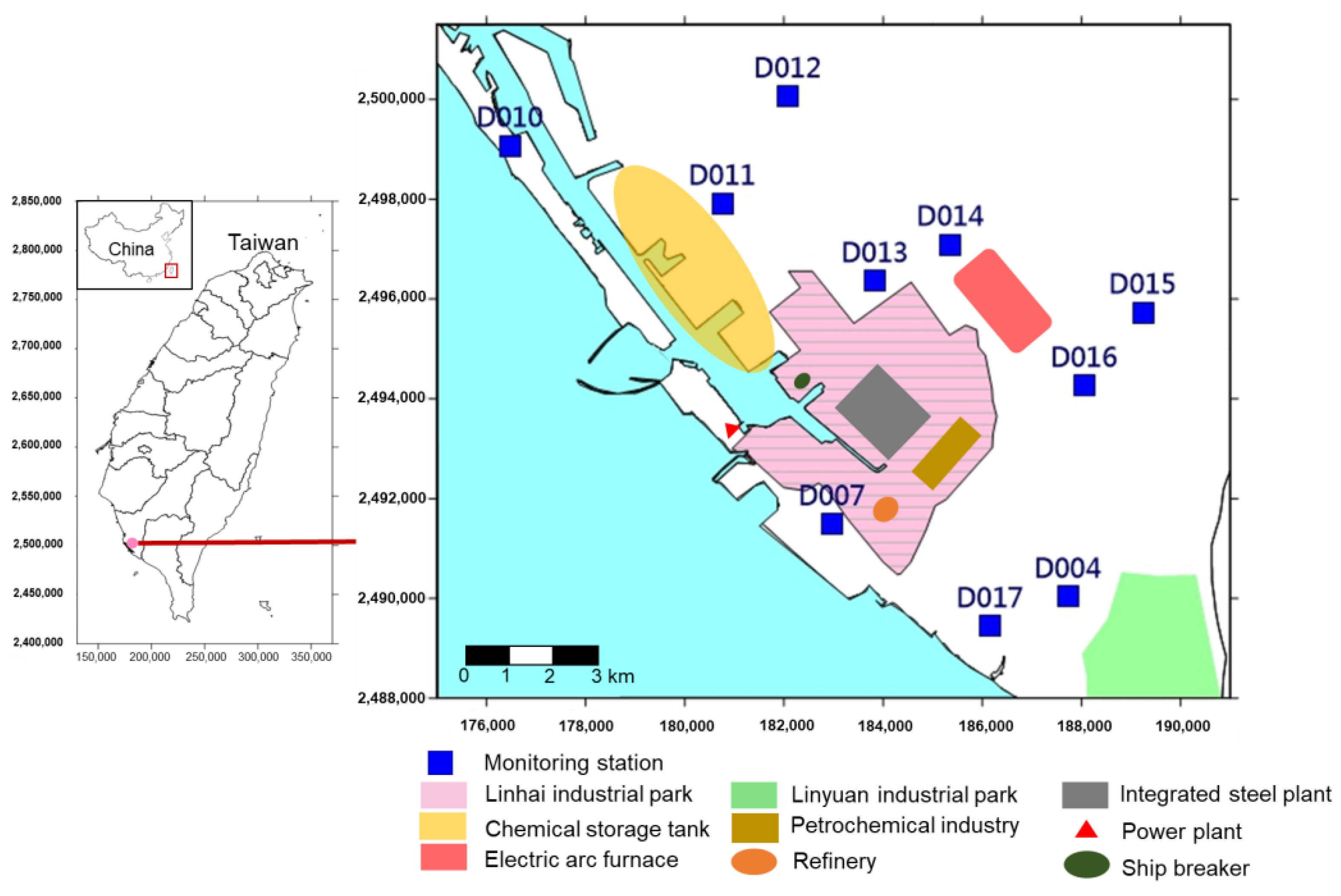
2.1. Study Area

In this study, we determined the airborne toxic emissions in the vicinity of Linhai industrial park in the Xiaogang district of Kaohsiung in Taiwan. Kaohsiung is the second-largest city in Taiwan and approximately 156,000 people live in the Xiaogang district. The area has a population density of more than 3400 people/km². The Xiaogang district is heavily industrialized; the Linhai industrial park has approximately 500 industrial facilities, approximately 40,000 people work in the park, and the output of the park contributes USD 33 billion to the economy.

The major processes in the Linhai industrial park include the manufacture of petroleum and coal products, the iron and steel industry, the aluminum refinery industry, ship-boat-diesel power generators, petrochemicals, chemical materials, and electronic parts and components. Kaohsiung port is also an area in which the traffic is dense (motor vehicles and airports). Figure 1 portrays the major sources of air pollution in the Xiaogang district.

2.2. Ambient Air-Monitoring Station

Figure 1 depicts ten ambient air monitoring stations that were used to determine the ambient air quality for the study area. The air toxin species mentioned in the US National Monitoring Programs’ annual report [1,9] and Taiwan’s list of hazardous air pollutants were considered in this study. A total of 54 ozone-precursor VOCs were determined by gas chromatography with flame ionization detection (GC-FID; auto GC-866, Chromatotec Group, Huston, TX, USA) [35], utilizing a two-column system: one system for the low carbon number (C2–C5) species and the other system for high carbon number (C6–C12) species.

VOCs and PM-bounded heavy metals were measured to evaluate the health risks accordingly.

(1)

In total, 71 VOCs (22 paraffins, 13 olefins, 13 carbonyls, 12 aromatics, 5 esters and ethers, and 6 other compounds) and 12 PM-bounded heavy metals were evaluated. The TO-15 and TO-17 (based on GC-FID analysis) [35,36,37] methods were used to monitor the VOC concentration every hour; thus, 24 data points per day and 8760 data points per year were collected;

(2)

In total, 52 HAP species were sampled every six days using the TO-15 method. The PM-bounded trace elements (nickel, arsenic, cadmium, magnesium, barium, and lead) were also measured every six days using the PM₁₀ sampler (Tisch TE-6070 PM₁₀ High Volume Air Sampler, OH, USA). The content of Cr(VI) in the total suspended particulate (TSP) was determined using the American society for testing and material (ASTM) [38] method. Benzo[a]pyrene (BaP) was sampled every 6 days and determined using the TO-13A [39] method.

The data for this study were acquired from 10 monitoring stations that collected 24-h integrated ambient air samples every 6days for 24 months. The samples were shipped to the TEPA-accredited laboratory for pollutant concentration analysis as follows:

(1)

Selected hydrocarbons, halogenated hydrocarbons, and polar compounds from canister samples for speciated non-methane organic compounds (SNMOCs) and/or VOCs were analyzed using the EPA Compendium TO-15 and TO-17 methods [35,36,37];

(2)

Carbonyl compounds from impinger samples were analyzed using the EPA compendium method TO-5 [40];

(3)

Trace metals (As. Pb, Mn, Cd, and Ni in PM₁₀) from filters were analyzed using the EPA compendium method IO-3.5/federal equivalency methods (FEM) EQL-0512-201 or EQL-0512-202;

(4)

Hexavalent chromium from sodium bicarbonate-coated filters (Cr(VI) in TSP) were analyzed using ASTM D7614 [38].

Based on the US EPA-approved quality assurance project plan (QAPP), the air monitoring station’s effective data were at least 85% complete. The data were used to calculate the monthly and annual mean concentrations and analyze the trends (ERG, 2015, 2016) [41,42]. This study utilized data from the air monitoring station that were more than 75% accurate to calculate the seasonal mean concentration. One sample every 6 days equates to 12 samples in one season; this indicated a quarterly mean concentration which was used to calculate the annual mean concentration.

2.3. Data Screening

In this study, 45 of the analyzed airborne pollutants had screening values. The species and their screening values are shown in Table S2. In order to determine the air pollutants in Linhai district, we followed the methods proposed by the NMP [1] for the screening procedures. On the other hand, the screening values were assigned using a risk-based screening method to evaluate the performance of the ambient air toxin monitoring datasets [43]. The cancer unit risk estimates (UREs) and non-cancer reference concentrations (RfCs) were used to estimate the cancer and non-cancer risks and to identify the HAP species and concentrations that posed a threat to human health. Furthermore, 28 species (will be presented below) that pose a cancer risk were analyzed using the NMP screening procedures. The screening procedures are shown in Figure S1.

Note that:

(1)

For the screening procedures, the cancer UREs and non-cancer RfCs were converted into screening values and the values were cited from the NMP [1,43];

(2)

Every preprocessed measurement was compared to the risk screening value with which it is associated. When the concentration was greater than the risk screening threshold, the incident was referred to as “failed the screen.”;

(3)

For each applicable pollutant, the number of failed screening procedures was tallied;

(4)

For each applicable pollutant, the percentage contribution of the failed screens to the overall number of the failed screens (program-wide) was calculated;

(5)

Pollutants of interest were defined as those that contributed to the top 95%of the overall number of failed screenings.

To include all the pollutants that contributed to the minimum 95% requirement for Step 5, the actual cumulative contribution may exceed 95% (shows a typical screening for the pollutant selection). If the cumulative threshold of 95% was met, but the pollutant contributed equally to the number of failed screens, it was also considered a pollutant of interest.

Using the NMP’s data screening techniques and the pollutant screening values of the NMP [43], the target pollutant screening values were determined by minimizing UREs and RfCs.

2.4. Emission Calculation

The emission sources were determined using the Taiwan emission data system (TEDS 10.0) [44] and updated every 2–3 years. According to TEDS 10.0, Kaohsiung’s PM₂.₅, SOx, NOx, hydrocarbon (HC), and CO, emissions in 2016 were 5708, 29,558, 45,630, 61,896, and 83,996 tonnes/year, respectively. The Xiaogang district accounted for 42% of the PM₂.₅, 76% of the SOx, 41% of the NOx, 10% of the HC, and 14% of the CO of the city of Kaohsiung’s air pollution emissions. The PM₂.₅ emissions are anticipated to amount to 53 tonnes/yr/km², 494 tonnes/yr/km² for SOx, 411 tonnes/yr/km² for NOx, 139 tonnes/yr/km² for HC, and 260 tonnes/yr/km² for CO. These emission loads indicate a heavy emission load in the Xiaogang district due to the presence of the Linhai industrial park, a heavily industrialized and densely populated urban neighborhood.

3. Results and Discussion

3.1. Method of Detection Limit (MDL) for Risk Assessment (Analytical Method)

In general, VOCs are determined using different analytical methods and detection limits. In this study, we tested the formaldehyde and acetaldehyde levels using the US EPA TO-5 method; the MDL level measured using the TO-5 method was higher than that measured using the TO-11 method [45]. The MDL calculated using the TO-5 method was approximately 40 times higher than that calculated using the TO-11 method. These results indicated that the differences in the sampling volume and quantitative volume for analysis could result in different MDL values for the two methods. A few previous studies indicate that the two methods are similar [46], while others suggest that using a cartridge is a better method for field monitoring and laboratory analysis [47]. We used the mean MDL for formaldehyde and acetaldehyde at the decade ppb level, which equated to thousands of NMP programs (shown in Table S3).

Notably, VOCs, such as benzene and ethylbenzene, were determined using gas chromatography–mass spectrometry (GC–MS) in the NMP program and GC-FID. The results indicated that the mean MDL for benzene and ethylbenzene calculated in this study was 4.4 and 6.1 times that calculated by the NMP, respectively. The MDL for other VOCs for different species ranged from 8 to 25 times the NMP program. The MDL was also high for the elements in PM, except for Ni, Pb, and Cr (VI).

The toxic concentrations for the majority of HAPs were less than the detection limit in ambient air; thus, a high MDL affected the health risk assessment [48]. A measurement of half of the MDL for the health risk assessment would eventually increase the health risk in the study location; therefore, the results for the health risk may not be accurate, which may be attributed to the analytical method, instrument, and technique applied for the assessments. The selection of an appropriate analysis methodology and monitoring program is crucial to determine the potential health risks due to environmental airborne pollution more accurately.

Table 1. Cancer risk determination for different species by 1/2 method of detection limit (MDL).

Compounds	Unit	Unit Risk Estimate (URE)	USEPA NMP *		Linhai Industrial Park
			1/2MDL-2015	1/2MDL-2016	1/2MDL-2017	1/2MDL-2018	1/2MDL-2019
Benzene	1/ppb	2.49 × 10−5	4.86 × 10−7	2.61 × 10−7	2.24 × 10−6	9.96 × 10−7	1.74 × 10−6
Ethylbenzene	1/ppb	1.85 × 10−5	1.76 × 10−7	1.76 × 10−7	1.57 × 10−6	8.33 × 10−7	8.33 × 10−7
Acetaldehyde	1/ppb	3.96 × 10−6	1.19 × 10−8	1.19 × 10−8	3.96 × 10−5	3.96 × 10−5	1.98 × 10−5
Formaldehyde	1/ppb	1.59 × 10−5	9.54 × 10−8	7.95 × 10−8	1.59 × 10−4	1.59 × 10−4	1.59 × 10−4
1,1,2,2-Tetrachloroethane	1/ppb	3.97 × 10−4	3.57 × 10−6	5.96 × 10−6	7.15 × 10−5	5.96 × 10−5	5.16 × 10−5
1,1,2-Trichloroethane	1/ppb	8.71 × 10−5	7.40 × 10−7	8.71 × 10−7	1.48 × 10−5	1.26 × 10−5	1.26 × 10−5
1,1-Dichloroethane	1/ppb	6.46 × 10−6	4.85 × 10−8	4.20 × 10−8	1.36 × 10−6	1.00 × 10−6	9.04 × 10−7
1,2-Dichloroethane	1/ppb	1.05 × 10−4	6.83 × 10−7	6.83 × 10−7	2.05 × 10−5	1.68 × 10−5	1.42 × 10−5
1,2-Dibromoethane	1/ppb	4.60 × 10−3	3.91 × 10−5	4.83 × 10−5	7.36 × 10−4	5.98 × 10−4	5.98 × 10−4
trans-1,3-Dichloropropene	1/ppb	1.81 × 10−5	1.90 × 10−7	2.44 × 10−7	2.81 × 10−6	1.99 × 10−6	1.99 × 10−6
cis-1,3-Dichloropropene	1/ppb	1.81 × 10−5	1.54 × 10−7	1.81 × 10−7	2.81 × 10−6	2.17 × 10−6	2.08 × 10−6
Carbon Tetrachloride	1/ppb	3.77 × 10−5	1.89 × 10−7	3.20 × 10−7	7.35 × 10−6	6.22 × 10−6	5.66 × 10−6
Chloroform	1/ppb	2.30 × 10−5	1.84 × 10−7	1.38 × 10−7	4.60 × 10−6	3.80 × 10−6	3.57 × 10−6
Dichloromethane	1/ppb	5.55 × 10−8	5.27 × 10−10	5.83 × 10−10	1.17 × 10−8	9.16 × 10−9	8.05 × 10−9
p-Dichlorobenzene	1/ppb	6.60 × 10−5	8.58 × 10−7	7.59 × 10−7	1.12 × 10−5	8.25 × 10−6	8.25 × 10−6
Trichloroethylene	1/ppb	2.57 × 10−5	2.18 × 10−7	2.18 × 10−7	4.37 × 10−6	3.86 × 10−6	3.98 × 10−6
Tetrachloroethylene	1/ppb	1.76 × 10−6	1.23 × 10−8	1.41 × 10−8	2.90 × 10−7	2.73 × 10−7	3.17 × 10−7
Vinyl chloride	1/ppb	2.24 × 10−5	8.96 × 10−8	3.58 × 10−7	4.59 × 10−6	3.14 × 10−6	2.80 × 10−6
1,3-Butadiene	1/ppb	6.62 × 10−5	4.63 × 10−7	8.61 × 10−7	1.39 × 10−5	9.27 × 10−6	8.61 × 10−6
Acrylonitrile	1/ppb	1.47 × 10−4	1.25 × 10−6	2.21 × 10−6	3.38 × 10−5	2.13 × 10−5	1.91 × 10−5
Hexachloro-1,3-Butadiene	1/ppb	2.34 × 10−4	3.98 × 10−6	4.91 × 10−6	4.45 × 10−5	3.16 × 10−5	3.16 × 10−5
Benzo[a]pyrene	1/ng/m3	1.76 × 10−6	1.16 × 10−7	5.54 × 10−8	6.69 × 10−7	6.86 × 10−7	7.92 × 10−8
As in PM10	1/ng/m3	4.30 × 10−6	1.23 × 10−7	2.80 × 10−8	1.29 × 10−7	1.08 × 10−7	1.29 × 10−7
Be in PM10	1/ng/m3	2.40 × 10−6	2.04 × 10−8	1.20 × 10−9	2.40 × 10−8	2.40 × 10−8	2.40 × 10−8
Cd in PM10	1/ng/m3	1.80 × 10−6	5.40 × 10−9	5.40 × 10−9	2.70 × 10−8	2.70 × 10−8	4.50 × 10−8
Ni in PM10	1/ng/m3	4.80 × 10−7	1.37 × 10−7	1.15 × 10−7	1.34 × 10−8	1.44 × 10−8	1.68 × 10−8
Pb in PM10	1/ng/m3	1.20 × 10−8	6.78 × 10−10	9.00 × 10−10	4.20 × 10−10	4.20 × 10−10	4.20 × 10−10
Cr(VI) in TSP	1/ng/m3	1.20 × 10−5	2.28 × 10−8	2.22 × 10−8	7.50 × 10−9	1.32 × 10−8	1.38 × 10−8
SUM	---	---	1.25 × 10−4	9.19 × 10−5	1.18× 10−3	9.81 × 10−4	9.47 × 10−4

* Note: United States environmental protection agency (USEPA) national monitoring program (NMP); total suspended particulate (TSP).

presents 28 HAPs that pose a risk of cancer. The results indicate that the concentration was equal to 1/2 MDL for 4 species (with a cancer risk higher than 10⁻⁶, in the NMP program) and 20 species (with a cancer risk higher than 10⁻⁶ in this study). We were able to determine the cancer risk for 20 species due to their high MDL (when compared to the NMP results).

3.2. Effect of the Number of Samples on Screening Species and the Effect of Data Integration and Data Weighting on Risk Assessment

This study collected 54 ozone precursor VOC species (each up to 8760 #/year-station) every hour (once every six days) to manually monitor the HAPs and BaP in PM and metal concentrations (approximately 60#/year-station) in PM. The sample size affected the screening species with less than 95% of failed data points. Our findings find that the screen may fail when the benzene and ethylbenzene levels are high; hence, the VOCs could be attributed to the failed fraction of the monitoring data (case A, Table S4)

For case B (Table S5), we used 24-h data to calculate the daily mean concentration (365#/year-station) and we assumed that the concentration of the metal (approximately 60#/year-station) in PM was the same for each group of six days. For case C (Table S6), we observed similar results for the 30-day mean for the concentrations of VOCs and PM-bounded metal (approximately 60#/year-station). For case D (Table S7), the 30-daily mean for the month provided a mean value for the ozone precursors VOCs and HAPs, for which the data were collected at six-day intervals, BaP in PM and metal concentration in PM (for the monthly data). For case D, all the species had 12 data points per year.

For case E (Table S8), the ozone precursors and VOC data were considered for a six-day mean, which is similar to the HAPs, benzo[a]pyrene in PM, and metal concentration in PM. Using the NMP screening procedures, the cumulative 95% failed species were considered the species of interest for the risk assessment. The results indicated that five cases had 2–12 health-risk species of interest.

In

Table 2. Cancer risk calculated for each case (cases A–E).

Group	A	B	C	D	E
Data type	Hourly data	Daily data	Monthly data	Monthly data for all	Every six-day one data for all
Benzene	78.10	2.26	1.60	2.38	2.06
Ethylbenzene	21.90	0.62	0.42	0.62	0.58
As		0.84	0.79	0.93	0.79
Ni		0.42	0.39	0.47	0.39
Formaldehyde		81.57	77.06	73.87	76.56
Pb		0.04	0.04	0.05	0.04
Cr(VI)		0.24	0.22	0.26	0.22
Cd		0.13	0.12	0.18	0.12
1,2-Dichloroethane		13.88	13.11	13.42	13.02
Vinyl chloride			1.40	1.80	1.39
Acetaldehyde			4.84	3.89	4.80
1,3-Butadiene				2.11
Screened Risk (1)	4.87 × 10−5	1.39 × 10−3	1.47 × 10−3	9.89 × 10−4	1.48 × 10−3
Total Risk (2)	1.58 × 10−3	1.57 × 10−3	1.56 × 10−3	1.03 × 10−3	1.57 × 10−3
Percentage (1/2) (%)	3.08	88.5	94.2	96.0	94.3

Note: Case A: Benzene and Ethylbenzene, hourly data (n = 251,740); others: every six-day accrue one data point (n = 1799), Case B: Benzene and Ethylbenzene, daily data (n = 10,487); others: every six-day accrue one data point (n = 1799), Case C: Benzene and Ethylbenzene, monthly data (n = 360); others: every six-day accrue one data point (n = 1799), Case D: Benzene and Ethylbenzene, monthly data (n = 360); others: monthly data (n = 360), Case E: Benzene, and Ethylbenzene, every 6 days to one data (n = 1820); others: every six-day accrue one data point (n = 1799).

, the cancer risk was determined by the different analyzed data integration (from hourly data to monthly data). The screening species were from two species for case A to 12 species for case D and the corresponding cancer risk was from 4.87 × 10⁻⁵ (case A) to1.48 × 10⁻³ (case E). The results reflected the total inhalation cancer risk from 3.5% in case A to 96% in case D. These results indicated that there was a large variation in the number of samples for different species and the screening procedures of the NMP; thus, the species of interest and health risk assessment provided misleading results. Therefore, we conclude that the design of the sampling program has a significant effect on the health risk assessment (Table 2).

Non-cancer risk (Table S9). For case A, benzene, ethylbenzene, and xylene were screened as the species of interest and the non-cancer risk was 0.27, which accounted for 1.8% of the total inhalation non-cancer risk. For case B-E, there were 11–14 selected species and the corresponding non-cancer risk was 9.18–15.20. In total, 66.5–97.7% of the total inhalation non-cancer risk was reflected. Results indicated the monthly average data (in case D) could miss high abundant variation to cause the underestimation of non-cancer risk.

3.3. Hazardous Air Pollutants (HAPs) in Ambient Concentrations

For the Linhai Industry Park, we selected the VOCs of interest and five metals (As, Be, Cd, Ni, and Pb) in PM₁₀ and Cr(VI) in TSP, using the reference concentration limits of WHO, and the data of Cr(VI) were collected using the NMP screening value.

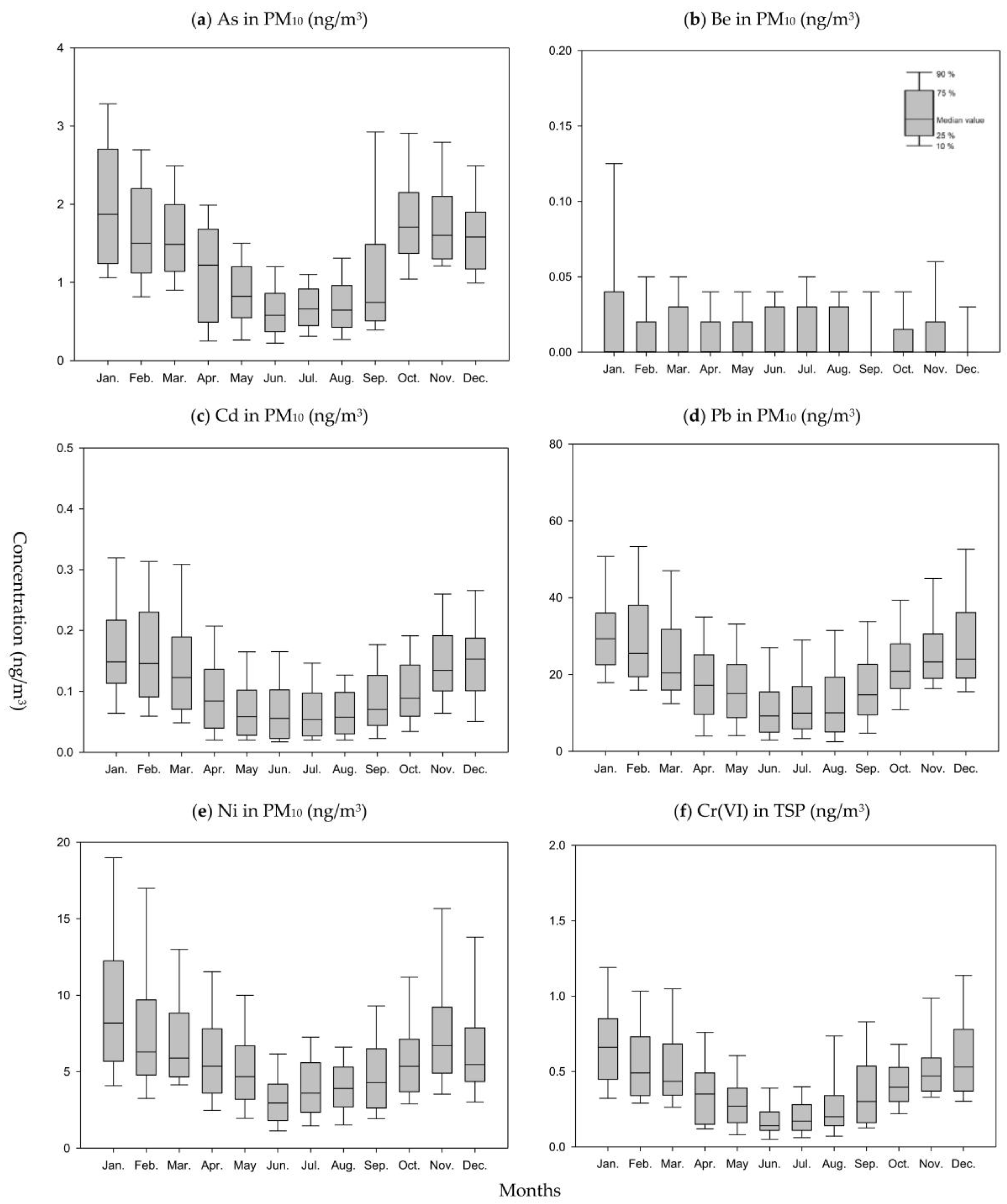
3.3.1. Elements in Particulate Matter (PM)

The elemental concentrations in PM are shown in

Table 3. Elemental hazardous air pollutant (HAP) concentrations during 2017–2019.

Compounds	2017	2018	2019	Average (2017–2019)	Summer	Winter
As in PM10	1.46 ± 0.90	1.20 ± 0.72	1.35 ± 1.16	1.34 ± 0.79	0.70 ± 0.41	1.77 ± 0.75
Be in PM10	0.02 ± 0.03	0.01 ± 0.02	0.02 ± 0.04	0.01 ± 0.02	0.01 ± 0.02	0.02 ± 0.04
Cd in PM10	0.51 ± 0.56	0.44 ± 0.49	0.43 ± 0.36	0.46 ± 0.27	0.27 ± 0.51	0.66 ± 0.44
Ni in PM10	7.87 ± 5.50	6.96 ± 5.54	4.35 ± 2.51	6.39 ± 3.16	4.11 ± 3.40	8.55 ± 5.92
Pb in PM10	24.08 ± 19.13	23.62 ± 32.20	22.26 ± 24.56	23.32 ± 1.94	15.40 ± 15.76	32.58 ± 23.54
Cr(VI) in TSP	0.13 ± 0.11	0.10 ± 0.14	0.13 ± 0.11	0.12 ± 0.07	0.08 ± 0.11	0.17 ± 0.15

Note: Unit: ng/m³; total suspended particulate (TSP).

. The concentration of As, Be, Cd, Ni, and Pb in PM₁₀ and of Cr(VI) was determined in the TSP. The mean respective As concentrations were 1.46 ± 0.90, 1.20 ± 0.72, and 1.35 ± 1.16 ng/m³ in 2017, 2018, and 2019, respectively (the high-mean to low-mean concentration ratio was 1.22 for the three years).

The Be concentrations were 0.02 ± 0.03, 0.01 ± 0.02, and 0.02 ± 0.04 ng/m³ in 2017, 2018, and 2019, respectively (the high-mean to low-mean concentration ratio was 1.74 for the three years). Most of the Be concentrations were below MDL.

The Cd concentrations were 0.51 ± 0.56, 0.44 ± 0.49, and 0.43 ± 0.36 ng/m³ in 2017, 2018, and 2019, respectively (the high-average to low-average concentration ratio was 1.19 for the three years).

The Pb concentrations were 24.08 ± 19.13 ng/m³ in 2017, 23.62 ± 32.20 ng/m³ in2018, and 22.26 ± 24.56 ng/m³ in2019 (the high-average to low-average concentration ratio was 1.08 for the three years).

The average Ni concentrations were 7.87 ± 5.50 ng/m³ in 2017, 6.96 ± 5.54 ng/m³ in 2018, and 4.35 ± 2.51 ng/m³ in 2019 (the high-average to low-average concentration ratio was 1.81 for the three years).

For Cr(VI) in TSP, the average concentrations were 0.13 ± 0.11 ng/m³ in 2017, 0.10 ± 0.14 ng/m³ in 2018, and 0.13 ± 0.11 ng/m³ in 2019 (the high-average to low-average concentration ratio was 1.30 for the three years). In terms of the heavy metal content in PM, the results indicated that the concentration of Ni decreased significantly from 2017 to 2019 but the concentrations of other elements did not portray this trend.

The combustion and production processing sites, including sinter plants, iron and steel industrial sites, non-ferrous metal industrial sites, organic chemical industrial sites, and road transport, were the sources of the metals in PM [49]. This aligns with past studies suggesting that industrial processes, fossil fuel combustion, and waste incineration release airborne Cu, Ni, Pb, and Cd. As, Ni, and Cr are the biggest cancer risks [50].

Findings of this study demonstrate variation in the pollutant concentrations in winter and summer. For instance, winter As concentrations were 1.77 ± 0.75 ng/m³, 2.53 times higher than the summer concentration. In winder, the mean concentration of Be was 0.02 ± 0.04 ng/m³ and 0.01 ± 0.02 ng/m³ in summer, which portrayed a two-fold difference. The mean concentration of Cd was 0.66 ± 0.44 ng/m³ in winter and 0.27 ± 0.51 ng/m³ in summer, which indicated a 2.44-fold difference. The mean concentration of Pb was 32.58 ± 23.54 ng/m³ in winter and 14.40 ± 15.76 ng/m³ in summer, which indicated a 2.26-fold difference. The mean concentration of Ni was 8.55 ± 5.92 ng/m³ in winter and 4.11 ± 3.40 ng/m3 in summer, which indicated a 2.08-fold difference. Finally, the mean concentration of Cr(VI) was 0.17 ± 0.15 ng/m³ in winter and 0.08 ± 0.11 ng/m³ in summer, which indicated a 2.12-fold difference. These results indicated that the metal content was highest in winter.

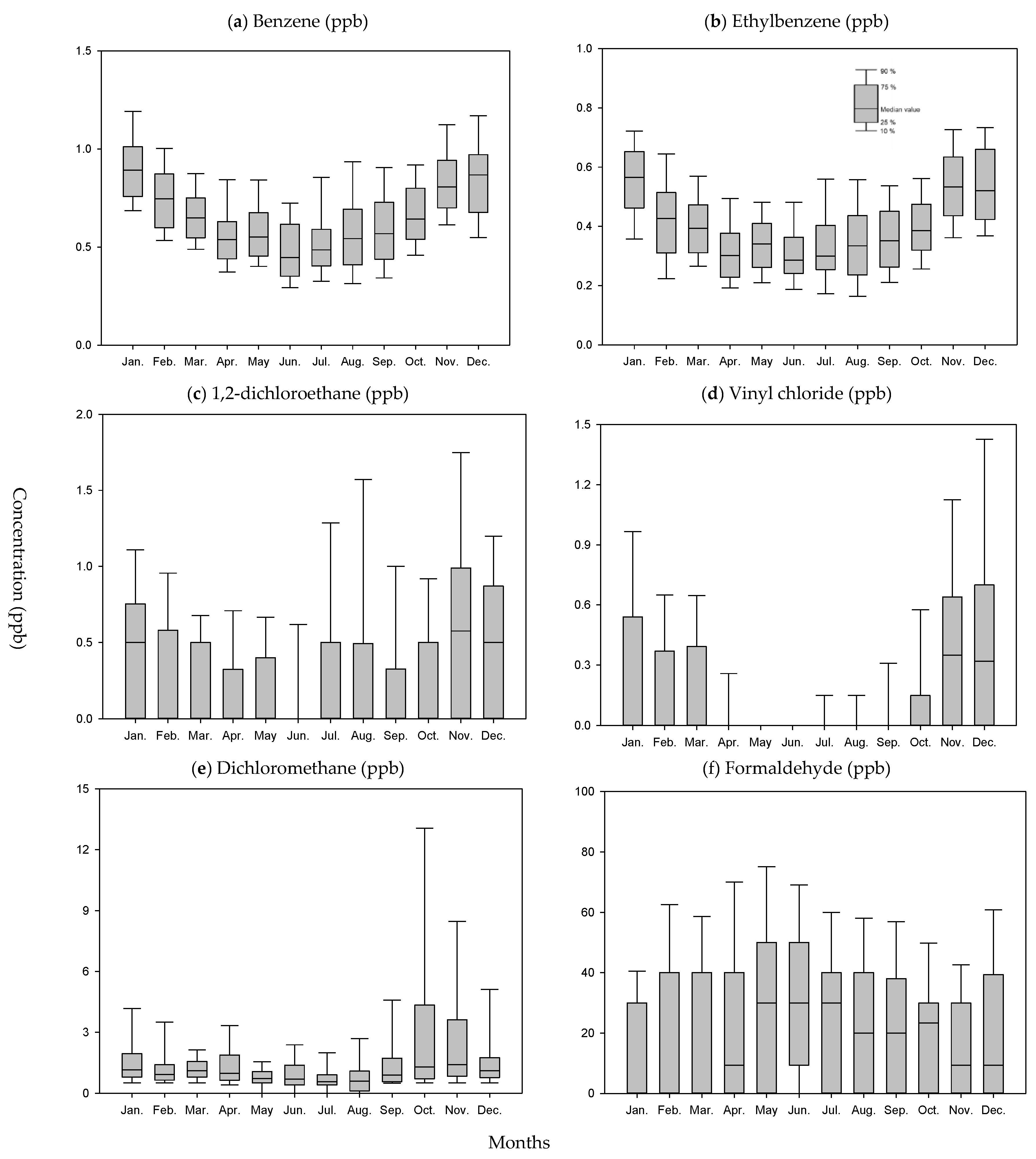
3.3.2. Organic Species in Ambient Conditions

The levels of organic hazardous air pollutants are shown in

Table 4. Organic hazardous air pollutants concentrations during 2017–2019 in the Linhai industrial park region.

Compounds	Unit	2017	2018	2019	2017–2019	Summer	Winter
Benzene	ppb	0.69 ± 0.47	0.73 ± 0.25	0.64 ± 0.24	0.69 ± 0.34	0.58 ± 0.51	0.85 ± 0.23
Ethylbenzene	ppb	0.39± 0.16	0.43 ± 0.17	0.41 ± 0.15	0.41 ± 0.16	0.33± 0.14	0.51 ± 0.16
Acetaldehyde	ppb	4.38 ± 9.33	0.75 ± 2.81	5.59± 11.60	3.56 ± 5.83	4.97± 10.83	2.48 ± 7.58
Formaldehyde	ppb	26.98 ± 29.30	20.62 ± 26.27	25.01 ± 30.33	24.12 ± 13.11	27.37 ± 25.43	20.54 ± 29.28
1,1-Dichloroethane	ppb	N.D.	0.001 ± 0.020	0.001 ± 0.013	0.000 ± 0.014	N.D.	N.D.
1,2-Dibromoethane	ppb	N.D.	N.D.	0.000 ± 0.006	0.000 ± 0.004	N.D.	N.D.
1,2-Dichloroethane	ppb	0.27 ± 0.65	0.31 ± 0.69	0.70 ± 1.86	0.43 ± 0.50	0.61± 2.17	0.45 ± 0.52
1,1,2-Thichloroethane	ppb	0.001 ± 0.017	0.000 ± 0.000	0.000 ± 0.006	0.000 ± 0.011	0.000 ± 0.000	0.001 ± 0.021
1,1,2,2-Tetrachloroethane	ppb	0.001 ± 0.020	N.D.	N.D.	0.000 ± 0.012	0.001 ± 0.024	0.000 ± 0.000
Carbon Tetrachloride	ppb	0.018 ± 0.142	0.008 ± 0.077	0.001 ± 0.021	0.009 ± 0.030	0.008 ± 0.089	0.012 ± 0.113
Chloroform	ppb	0.018 ± 0.165	0.033 ± 0.131	0.045 ± 0.134	0.032 ± 0.059	0.018 ± 0.110	0.063 ± 0.209
Dichloromethane	ppb	2.89 ± 5.04	1.41 ± 2.52	1.47 ± 2.43	1.93 ± 2.52	1.15 ± 2.47	2.01 ± 3.35
p-Dichlorobenzene	ppb	N.D.	0.001 ± 0.020	N.D.	0.000 ± 0.012	0.001 ± 0.019	N.D.
Tetrachloroethylene	ppb	0.001 ± 0.017	0.049 ± 0.482	N.D.	0.017 ± 0.162	N.D.	0.065 ± 0.566
Trichloroethylene	ppb	0.001 ± 0.017	N.D.	N.D.	0.000 ± 0.010	N.D.	0.001 ± 0.020
Vinyl chloride	ppb	0.26 ± 2.10	0.18 ± 0.53	0.25 ± 0.47	0.23 ± 0.47	0.19 ± 2.39	0.35 ± 0.59
1,3-Butadiene	ppb	0.05± 0.20	0.11± 0.36	0.11 ± 0.25	0.09± 0.16	0.03 ± 0.16	0.17 ± 0.35
Acrylonitrile	ppb	0.06 ± 0.33	0.06 ± 0.26	0.05 ± 0.17	0.05± 0.14	0.02 ± 0.22	0.12 ± 0.41
Hexachloro-1,3-butadiene	ppb	0.002 ± 0.031	N.D.	0.000 ± 0.012	0.001 ± 0.019	0.002 ± 0.029	0.000 ± 0.000
Benzo[a]pyrene	ng/m3	0.04 ± 0.16	0.04± 0.18	0.09± 0.19	0.06 ± 0.07	0.03 ± 0.07	0.09 ± 0.17

Note: cis-1,3-Dichloropropene and trans-1,3-Dichloropropene are not detectable(ND)during 2017–2019.

. The average formaldehyde concentration was 26.98 ± 29.30 ppb in 2017, 20.62 ± 26.27 ppb in 2018, and 25.01 ± 30.32 ppb in 2019 (the high-average to low-average concentration ratio was 1.31 for the three years).

Acetaldehyde’s mean concentration was 4.38 ± 9.33 ppb in 2017, 0.75 ± 2.81 ppb in 2018, and 5.59 ± 11.60 ppb in 2019 (the high-mean to low-mean concentration ratio was 7.45 for the three years). The winter formaldehyde concentration was 20.54 ± 29.28 ppb and the summer concentration was 27.37 ± 25.43 ppb, which indicated a 1.27-fold difference. The winter acetaldehyde concentration was 2.48 ± 7.58 ppb and the summer concentration was 4.97 ± 10.83 ppb, which stated a 1.55-fold difference. Since primary emissions from combustion sources are a significant contributor to ambient formaldehyde in urban environments, with motor vehicles being the most important source, the formaldehyde and acetaldehyde concentrations were significantly higher in the summer due to photochemical reactions [51,52,53,54].

Acrylonitrile’s mean concentration was 0.06 ± 0.33 ppb in 2017, 0.06 ± 0.26 ppb in 2018, and 0.05 ± 0.17 ppb in 2019 (the high-mean and low-mean concentration ratio was 1.08 for the three years). The mean 1.3-butadiene concentration was 0.05 ± 0.20 ppb in 2017, 0.11 ± 0.36 ppb in 2018, and 0.11 ± 0.25 ppb in 2019 (the high-mean and low-mean concentration ratio was 1.33 for the three years).

The mean concentration of acetonitrile was 2.50 ± 0.24 ppb in winter and 2.59 ± 0.06 ppb in summer, which indicated a 1.04-fold difference. The mean concentration of acrylonitrile was 0.12 ± 0.24 ppb in winter and 0.02 ± 0.06 ppb in summer, which stated a 6.0-fold difference. The mean concentration of 1.3-Butadiene was 0.17 ± 0.35 ppb in winter and 0.03 ± 0.16 ppb in summer, which indicated a 5.67-fold difference.

The acrylonitrile and 1.3-butadiene were higher in winter; this was not true for acetonitrile. These results indicate a significant difference in the concentration of acrylonitrile and 1.3-butadiene but none for acetonitrile.

The mean concentration of 1,2-dichloroethane was 0.27 ± 0.65 ppb in 2017, 0.31 ± 0.69 ppb in 2018, and 0.70 ± 1.86 ppb in 2019 (the high-mean and low-mean concentration ratio was 2.59 for the three years). The mean concentration of vinyl chloride was 0.26 ± 2.10 ppb in 2017, 0.18 ± 0.53 ppb in 2018, and 0.25 ± 0.47 ppb in 2019 (the high-mean and low-mean concentration ratio was 1.46 for the three years).

Furthermore, the mean concentration of dichloromethane was 2.89 ± 5.04 ppb in 2017, 1.41 ± 2.52 ppb in 2018, and 1.47 ± 2.43 ppb in 2019 (the high-mean and low-mean concentration ratio was 2.05 for the three years). The mean concentration of chloromethane was 0.94 ± 0.42 ppb in 2017, 1.02 ± 0.31 ppb in 2018, and 1.02 ± 0.39 ppb in 2019 (the high-mean and low-mean concentration ratio was 1.08 for the three years).

The mean concentration of dichloroethane was 0.44 ± 0.52 ppb in winter and 0.61 ± 2.17 ppb in summer; thus, the mean concentration was slightly higher in summer. The mean concentration of vinyl chloride was 0.35 ± 0.59 ppb in winter and 0.19 ± 2.35 ppb in summer (thus, the concentration was higher in winter). The mean concentration of dichloromethane was 2.00 ± 3.35 ppb in winter and 1.15 ± 2.47 ppb in summer. Notably, the concentrations of 1,2-dichloroethane, vinyl chloride, and chloromethane were higher in summer.

Regarding aromatic species, the mean benzene concentration was 0.69 ± 0.47 ppb in 2017, 0.73 ± 0.25 ppb in 2018, and 0.64 ± 0.24 ppb in 2019 (the high-mean and low-mean concentration ratio was 1.14 for the three years). The mean concentration of ethylbenzene was 0.39 ± 0.16 ppb in 2017, 0.43 ± 0.17 ppb in 2018, and 0.41 ± 0.15 ppb in 2019 (the high-mean and low-mean concentration ratio was 1.10 for the three years). Thus, the difference in the mean concentration from 2017 to 2019 was insignificant.

The mean concentration of benzene was 0.85 ± 0.23 ppb in winter and 0.58 ± 0.51 ppb in summer, which indicated a 1.46-fold difference. The mean ethylbenzene concentration was 0.51 ± 0.16 ppb in winter and 0.33 ± 0.14 ppb in summer, indicating a 1.54-fold difference.

The mean concentrations of the aromatic species were approximately 50% higher in winter than in summer. In general, there is a high mean concentration of total volatile organic compounds (TVOC) in winter (32.54 ppb) and a low TVOC concentration in summer (25.84 ppb) [50]. Toluene and m,p-xylenes are the precursors with the greatest potential to form ozone by photochemical reactions [55].

The sequence of the estimated carcinogenic risks is 1,2-dichloroethane, benzene, chloroform, and carbon tetrachloride, and in a heavily industrialized region, the risk is substantially higher than the acceptable level [56]. The VOC species are present at significantly higher levels in winter than in summer, except for isoprene [57]. The carcinogenic risks for carbon tetrachloride, benzene, 1,3-butadiene, and naphthalene are considered as 10^-5-10^-4 [57].

3.3.3. Temporal Distribution

Figure 2 portrays the variations in the concentration of organic species in ambient air based on our analysis.

In terms of aromatic species, the monthly average concentration of ethylbenzene ranged from 0.31 ppb (June) to 0.55 ppb (January). The average concentration of benzene ranged from 0.51 ppb (June) to 0.92 ppb (January).

In terms of the chlorinated species, the average monthly concentration of 1,2-dichloroethane ranged from 0.20 ppb (May) to 0.89 ppb (July), indicating a high-average to low-average concentration ratio of 4.45. The average concentration of vinyl chloride varied from 0.05 ppb (April and May) to 0.53 ppb (December) (the high-average to low-average concentration ratio was 10.6). The average concentration of chloromethane varied from 0.67 ppb (July) to 1.37 ppb (January) (high-average to low-average concentration ratio was 2.04). The average concentration of chloroform varied from 0.01 ppb (June and August) to 0.08 ppb (January) (high-average to low-average concentration ratio was 8.0). The concentration of tetrachloroethene was low and most samples indicated no presence.

In terms of formaldehyde and acetaldehyde, the mean monthly concentration of formaldehyde varied from 17.88 ppb (January) to 32.27 ppb (June), indicating a high-mean to low-mean concentration ratio of 1.80. The mean concentration of acetaldehyde varied from 1.13 ppb (February) to 5.24 ppb (July) (indicating a high-mean to low-mean concentration ratio of 4.64).

In terms of acetonitrile, acrylonitrile, and 1.3-butadiene, the mean concentration of acetonitrile varied from 1.73 ppb (December) to 4.27 ppb (April) (indicating a high-mean to low-mean concentration ratio of 2.47). The mean monthly concentration of acrylonitrile varied from 0.01 ppb (March and September) to 0.18 ppb (January), indicating a high-mean to low-mean concentration ratio of 18.0.

In terms of the elements in PM, Figure 3 portrays the variety of elements in the atmosphere in different months. The average concentration of arsenic varied from 0.66 ng/m³ (June) to 2.02 ng/m³ (January) (indicating a high-average to low-average concentration ratio of 3.06). The average monthly concentration of Be was 0.01 ng/m³ (from April to October) to 0.03 ng/m³ (January); therefore, there was little variation in the concentration of Be in PM₁₀.

The average concentration of lead varied from 13.31 ng/m³ (July) to 32.74 ng/m³ (January) (indicating a high-average to low-average concentration ratio of 2.46). The average concentration of Mn varied from 15.91 ng/m³ (May) to 44.01 ng/m³ (November) (indicating a high-average to low-average concentration ratio of 2.77). The average concentration of Cd varied from 0.21 ng/m³ (June) to 0.71 ng/m³ (January) (indicating a high-average to low-average concentration ratio of 3.38). The average concentration of Ni varied from 3.39 ng/m³ (June) to 9.83 ng/m³ (January) (indicating a high-average to low-average concentration ratio of 2.90). The average concentration of Cr(VI) varied from 0.07 ng/m³ (June and August) to 0.18 ng/m³ (December) (indicating a high-average to low-average concentration ratio of 2.57).

3.3.4. Spatial Distribution

Figures S2 and S3 portrays the elemental spatial distribution on an annual and seasonal basis. The spatial distribution of the mean concentration of ethylbenzene was 0.31–0.52 ppb and benzene was 0.50–0.94 ppb.

In terms of the chlorinated species, the concentration of dichloroethane was 0.22–1.20 ppb and dichomomethane was 0.94–2.33 ppb. The concentration of tetrachoroethylene was high in location D014 (0–0.07 ppb) and that of chloroethene was 0.12–0.33 ppb; the concentration of chloromethane was 0.82–1.20 ppb and chloroform was 0.00–0.14 ppb.

The concentration of 1,3-butadiene was 0.04–0.14 ppb, acetonitrile was 1.18–4.05 ppb, acrylonitrile was 0.003–0.108 ppb, formaldehyde was 14.92–47.91 ppb, and acetaldehyde was 2.28–4.72 ppb.

In PM₁₀, the arsenic concentration was 1.15–1.66 ng/m³ and the concentration of beryllium was 0.007–0.030 ng/m³ and that of lead was 15.90–31.96 ng/m³.Manganese was 17.87–47.82 ng/m³ and nickel was 4.57–11.73 ng/m³. In TSP, the concentration of Cr(VI) was 0.07–0.16 ng/m³ and the concentration of BaP was 0.01–0.22 ng/m³.

The results indicated that there was a benzene hotspot in the vicinity of D007 and that the emission source could be a coke-oven process in the iron and steel plant that is upwind or from the petrochemical industry emissions inland (toward the downtown area). Ethylbenzene was emitted from the paint process for naval architecture in the industrial park and from the petrochemical plants that surrounded the industrial park in the northeast (D0015). Dichloroethane was emitted from the vinyl chloride manufacturing plant and the petrochemical plants in the southwestern area; the concentrations were higher in the summer, due to the vaporization of liquids in storage tanks near the harbor and the fugitive sources from an industrial facility, which was similar to the results of a previous study [41].

Highlyabundant metals were determined in winter to compare their presence to thatin summer. In addition, high As, Cd, Pb, and Ni concentrations were located in the vicinity of D007 and D017. The metal smelting industries could be the sources of toxic metals in particulate matter. The Cr(VI) concentration was high inland and low in the vicinity coast, therefore, Cr(VI) may not come from the facility of Linhai industrial park.

4. Conclusions

Hazardous air pollutants (HAPs) affect environmental air quality significantly and are thus analyzed to determine the health risks to humans; in this study, we determined that species, sampling frequency, and data-screening procedures are crucial for obtaining comprehensive and representative information.

We propose that the MDL for analysis methods and the sampling frequency for different species (and the species of interest) affect the results of health risk assessments; thus, the current control strategies for the reduction in health risks may not be effective. Our results indicated that in the Linhai industrial park, formaldehyde, 1,2-dichloroethane, acetaldehyde, benzene, vinyl chloride, As, ethylbenzene, Ni, Cr(VI), Cd, Pb, and 1,3-butadiene are the high-risk species. Notably, VOCs accounted for more than 95% of the health risks associated with the respiratory system.

Additionally, we observed that formaldehyde production processes emitted high-risk fractions of VOC formaldehyde and the urea-formaldehyde resin process was a key source of formaldehyde. 1,2-dichloroethane was also emitted by the vinyl chloride production facility near the industrial park (to the south). The iron and steel facility in the industrial park and the electrical arc furnaces in ferrous and non-ferrous industries were the major sources of metals in ambient PM.

References

1. USEPA. United States Environmental Protection Agency 2015–2016. National Monitoring Programs Annual Report (UATMP, NATTS, and CSATAM); EPA Contract No. EP-D-14-030; USEPA: Washington, DC, USA, 2018. [Google Scholar]
2. WHO—Word Health Organization Regional Office for Europe; OECD. Economic Cost of the Health Impact of Air Pollution in Europe: Clean Air, Health and Wealth; WHO Regional Office for Europe: Copenhagen, Denmark, 2015. [Google Scholar]
3. Environmental Protection Agency. What are Hazardous Air Pollutants? 2020. Available online: https://www.epa.gov/haps/what-are-hazardous-air-pollutants (accessed on 6 January 2020).
4. United States Environmental Protection Agency. Volatile Organic Compounds Impact on Indoor Air Quality. 2017. Available online: https://www.epa.gov/indoor-air-quality-iaq/volatile-organic-compounds-impact-indoor-air-quality#Health_Effects (accessed on 15 May 2021).
5. Robichaud, A. An overview of selected emerging outdoor airborne pollutants and air quality issues: The need to reduce uncertainty about environmental and human impacts. J. Air Waste Manag. Assoc. 2020, 70, 341–378. [Google Scholar] [CrossRef] [PubMed]
6. IARC. International Agency for Research on Cancer. Monographs on the Identification of Carcinogenic Hazards to Humans. 2019. Available online: https://monographs.iarc.fr/list-of-classifications-volumes/ (accessed on 20 May 2019).
7. The Government of the Hong Kong. Environmental Protection Department. Hong Kong Air Pollutant Emission Inventory—Volatile Organic Compounds. Available online: https://www.epd.gov.hk/epd/english/environmentinhk/air/data/emission_inve.html (accessed on 16 May 2021).
8. CE Delft. Health Impacts and Costs of Diesel Emissions in the EU; CE Delft: Delft, The Netherlands, 2018. [Google Scholar]
9. Southern Coast Air Quality Management District (SCAQMD). Multiple Air Toxics Exposure Study IV (MATES IV); Final Report; SCAQMD: Diamond Bar, CA, USA, 2015. [Google Scholar]
10. Wang, M.; Qin, W.; Chen, W.; Zhang, L.; Zhang, Y.; Zhang, X.; Xie, X. Seasonal variability of VOCs in Nanjing, Yangtze River delta: Implications for emission sources and photochemistry. Atmos. Environ. 2020, 223, 117254. [Google Scholar] [CrossRef]
11. Zhou, X.; Peng, X.; Montazeri, A.; McHale, L.E.; Gaßner, S.; Lyon, D.R.; Yalin, A.P.; Albertson, J.D. Mobile Measurement System for the Rapid and Cost-Effective Surveillance of Methane and Volatile Organic Compound Emissions from Oil and Gas Production Sites. Environ. Sci. Technol. 2020, 55, 581–592. [Google Scholar] [CrossRef] [PubMed]
12. Chen, C.H.; Chuang, Y.C.; Hsieh, C.C.; Lee, C.S. VOC characteristics and source apportionment at a PAMS site near an industrial complex in central Taiwan. Atmos. Pollut. Res. 2019, 10, 1060–1074. [Google Scholar] [CrossRef]
13. Xuan, L.; Ma, Y.; Xing, Y.; Meng, Q.; Song, J.; Chen, T.; Wang, H.; Wang, P.; Zhang, Y.; Gao, P. Source, temporal variation and health risk of volatile organic compounds (VOCs) from urban traffic in Harbin, China. Environ. Pollut. 2021, 270, 116074. [Google Scholar] [CrossRef]
14. Song, M.; Li, X.; Yang, S.; Yu, X.; Zhou, S.; Yang, Y.; Chen, S.; Dong, H.; Liao, K.; Chen, Q.; et al. Spatiotemporal variation, sources, and secondary transformation potential of volatile organic compounds in Xi’an, China. Atmos. Meas. Tech. 2021, 21, 4939–4958. [Google Scholar] [CrossRef]
15. Xiong, Y.; Du, K. Source-resolved attribution of ground-level ozone formation potential from VOC emissions in Metropolitan Vancouver, BC. Sci. Total Environ. 2020, 721, 137698. [Google Scholar] [CrossRef]
16. USEPA—United States Environmental Protection Agency. Cancer Risk from Outdoor Exposure to Air Toxics; EPA-450/1-90-004a; USEPA: Washington, DC, USA, 1990. [Google Scholar]
17. Lyu, X.; Guo, H.; Wang, Y.; Zhang, F.; Nie, K.; Dang, J.; Liang, Z.; Dong, S.; Zeren, Y.; Zhou, B.; et al. Hazardous volatile organic compounds in ambient air of China. Chemosphere 2020, 246, 125731. [Google Scholar] [CrossRef]
18. Li, B.; Ho, S.S.H.; Qu, L.; Gong, S.; Ho, K.F.; Zhao, D.; Qi, Y.; Chan, C.S. Temporal and spatial discrepancies of VOCs in an industrial-dominant city in China during summertime. Chemosphere 2021, 264, 128536. [Google Scholar] [CrossRef]
19. Tan, Y.; Han, S.; Chen, Y.; Zhang, Z.; Li, H.; Li, W.; Yuan, Q.; Li, X.; Wang, T.; Lee, S.-C. Characteristics and source apportionment of volatile organic compounds (VOCs) at a coastal site in Hong Kong. Sci. Total. Environ. 2021, 777, 146241. [Google Scholar] [CrossRef]
20. Cheng, N.; Jing, D.; Zhang, C.; Chen, Z.; Li, W.; Li, S.; Wang, Q. Process-based VOCs source profiles and contributions to ozone formation and carcinogenic risk in a typical chemical synthesis pharmaceutical industry in China. Sci. Total. Environ. 2021, 752, 141899. [Google Scholar] [CrossRef] [PubMed]
21. Gao, Y.; Li, M.; Wan, X.; Zhao, X.; Wu, Y.; Liu, X.; Li, X. Important contributions of alkenes and aromatics to VOCs emissions, chemistry and secondary pollutants formation at an industrial site of central eastern China. Atmos. Environ. 2021, 244, 117927. [Google Scholar] [CrossRef]
22. Zheng, H.; Kong, S.; Yan, Y.; Chen, N.; Yao, L.; Liu, X.; Wu, F.; Cheng, Y.; Niu, Z.; Zheng, S.; et al. Compositions, sources and health risks of ambient volatile organic compounds (VOCs) at a petrochemical industrial park along the Yangtze River. Sci. Total. Environ. 2020, 703, 135505. [Google Scholar] [CrossRef] [PubMed]
23. Alias, N.F.; Khan, M.F.; Sairi, N.A.; Zain, S.M.; Suradi, H.; Rahim, H.A.; Banerjee, T.; Bari, M.A.; Othman, M.; Latif, M.T. Characteristics, emission sources, and risk factors of heavy metals in PM2.5 from Southern Malaysia. ACS Earth Space Chem 2020, 4, 1309–1323. [Google Scholar] [CrossRef]
24. Li, F.; Yan, J.; Wei, Y.; Zeng, J.; Wang, X.; Chen, X.; Zhang, C.; Li, W.; Chen, M.; Lü, G. PM2.5-bound heavy metals from the major cities in China: Spatiotemporal distribution, fuzzy exposure assessment and health risk management. J. Clean. Prod. 2021, 286, 124967. [Google Scholar] [CrossRef]
25. Zhou, X.; Strezov, V.; Jiang, Y.; Yang, X.; Kan, T.; Evans, T. Contamination identification, source apportionment and health risk assessment of trace elements at different fractions of atmospheric particles at iron and steelmaking areas in China. PLoS ONE 2020, 15, e0230983. [Google Scholar] [CrossRef]
26. Men, C.; Wang, Y.; Liu, R.; Wang, Q.; Miao, Y.; Jiao, L.; Shoaib, M.; Shen, Z. Temporal variations of levels and sources of health risk associated with heavy metals in road dust in Beijing from May 2016 to April 2018. Chemosphere 2021, 270, 129434. [Google Scholar] [CrossRef]
27. Ramírez, O.; de la Campa AM, S.; Sánchez-Rodas, D.; de la Rosa, J.D. Hazardous trace elements in thoracic fraction of airborne particulate matter: Assessment of temporal variations, sources, and health risks in a megacity. Sci. Total Environ. 2020, 710, 136344. [Google Scholar] [CrossRef]
28. Kolakkandi, V.; Sharma, B.; Rana, A.; Dey, S.; Rawat, P.; Sarkar, S. Spatially resolved distribution, sources and health risks of heavy metals in size-fractionated road dust from 57 sites across megacity Kolkata, India. Sci. Total. Environ. 2020, 705, 135805. [Google Scholar] [CrossRef]
29. Xu, J.; White, A.J.; Niehoff, N.M.; O’Brien, K.M.; Sandler, D.P. Airborne metals exposure and risk of hypertension in the Sister Study. Environ. Res. 2020, 191, 110144. [Google Scholar] [CrossRef]
30. Schiavo, B.; Meza-Figueroa, D.; Vizuete-Jaramillo, E.; Robles-Morua, A.; Angulo-Molina, A.; Reyes-Castro, P.A.; Inguaggiato, C.; Gonzalez-Grijalva, B.; Pedroza-Montero, M. Oxidative potential of metal-polluted urban dust as a potential environmental stressor for chronic diseases. Environ. Geochem. Health 2023, 45, 3229–3250. [Google Scholar] [CrossRef]
31. Das, A.; Habib, G.; Perumal, V.; Kumar, A. Estimating seasonal variations of realistic exposure doses and risks to organs due to ambient particulate matter-bound metals of Delhi. Chemosphere 2020, 260, 127451. [Google Scholar] [CrossRef]
32. Hao, Y.; Luo, B.; Simayi, M.; Zhang, W.; Jiang, Y.; He, J.; Xie, S. Spatiotemporal patterns of PM2.5 elemental composition over China and associated health risks. Environ. Pollut. 2020, 265, 114910. [Google Scholar] [CrossRef] [PubMed]
33. Parvizimehr, A.; Baghani, A.N.; Hoseini, M.; Sorooshian, A.; Cuevas-Robles, A.; Fararouei, M.; Dehghani, M.; Delikhoon, M.; Barkhordari, A.; Shahsavani, S.; et al. On the nature of heavy metals in PM10 for an urban desert city in the Middle East: Shiraz, Iran. Microchem. J. 2020, 154, 104596. [Google Scholar] [CrossRef]
34. Xie, J.-J.; Yuan, C.-G.; Xie, J.; Niu, X.-D.; Zhang, X.-R.; Zhang, K.-G.; Xu, P.-Y.; Ma, X.-Y.; Lv, X.-B. Comparison of arsenic fractions and health risks in PM2.5 before and after coal-gas replacement. Environ. Pollut. 2020, 259, 113881. [Google Scholar] [CrossRef] [PubMed]
35. USEPA—United States Environmental Protection Agency. Compendium Method TO-15 for the Determination of Volatile Organic Compounds (VOCs) in Air Collected in Specially Prepared Canisters and Analyzed by Gas Chromatography/Mass Spectrometry (GC/MS); United States Environmental Protection Agency: Washington, DC, USA, 1999. [Google Scholar]
36. USEPA—United States Environmental Protection Agency. Determination of Volatile Organic Compounds (VOCs) in Air Collected in Specially Prepared Canisters and Analyzed by Gas Chromatography-Mass Spectrometry (GC-MS); Method TO-15A; United States Environmental Protection Agency: Washington, DC, USA, 2019. [Google Scholar]
37. USEPA—United States Environmental Protection Agency. Compendium Method TO-17 for the Determination of Volatile Organic Compounds (VOCs) in Air Using Active Sampling onto Sorbent Tubes; United States Environmental Protection Agency: Washington, DC, USA, 1999. [Google Scholar]
38. ASTM D7614; Standard Test Method for Determination of Total Suspended Particulate (TSP) Hexavalent Chromium in Ambient Air Analyzed by Ion Chromatography (IC) and Spectrophotometric Measurements. ASTM: West Conshohocken, PA, USA. Available online: https://www.astm.org/d7614-20.html (accessed on 5 October 2020).
39. USEPA—United States Environmental Protection Agency. Compendium of Methods for the Determination of Toxic Organic Compounds in Ambient Air, The Determination of Benzo(a)pyrene (B(a)P) and other Polynuclear Aromatic Hydrocarbons (PAHs) in the Ambient Air Using Gas Chromatographic (GC) and High Performance Liquid Chromatographic (HPLC) Analysis; Method 13; United States Environmental Protection Agency: Washington, DC, USA, 1989. [Google Scholar]
40. USEPA—United States Environmental Protection Agency. Compendium Method TO-5, Determination of Aldehydes and Ketones in Ambient Air Using High Performance Liquid Chromatography (HPLC); United States Environmental Protection Agency: Washington, DC, USA, 1984. [Google Scholar]
41. ERG—Eastern Research Group, Inc. Support for the EPA National Monitoring Programs (UATMP, NATTS, CSATAM, PAMS, and NMOC Support), Quality Assurance Project Plan, Category 1; Contract No. EP-D-14-030; ERG: Morrisville, NC, USA, 2015. [Google Scholar]
42. ERG—Eastern Research Group, Inc. Support for the EPA National Monitoring Programs (UATMP, NATTS, CSATAM, PAMS, and NMOC Support), Quality Assurance Project Plan, Category 1; Contract No. EP-D-14-030; ERG: Morrisville, NC, USA, 2016. [Google Scholar]
43. USEPA—United States Environmental Protection Agency. A Preliminary Risk-based Screening Approach for Air Toxics Monitoring Data Sets; version 2; EPA-904-B-06-001; USEPA: Atlanta, GA, USA, 2010. Available online: nepis.epa.gov/Exe/ZyPURL.cgi?Dockey=P1009A7C (accessed on 7 May 2022).
44. Taiwan Environmental Protection Agency (TEPA). Taiwan Air Pollutants Emission Data System. 2021. Available online: https://teds.epa.gov.tw/Introduction.aspx (accessed on 26 August 2021).
45. USEPA—United States Environmental Protection Agency. Compendium Method TO-11A, Determination of Formaldehyde in Ambient Air Using Adsorbent Cartridge Followed by High Performance Liquid Chromatography (HPLC); USEPA: Washington, DC, USA, 1999. [Google Scholar]
46. Tejada, S.B. Evaluation of silica gel cartridges coated in situ with acidified 2, 4-Dinitrophenylhydrazine for sampling aldehydes and ketones in air. Int. J. Environ. Anal. Chem. 1986, 26, 167–185. [Google Scholar] [CrossRef]
47. Ferrari, C.P.; Durand-Jolibois, R.; Carlier, P.; Jacob, V.; Roche, A.; Foster, P.; Fresnet, P. Comparison between two carbonyl measurement methods in the atmosphere. Analysis 1999, 27, 45–53. [Google Scholar] [CrossRef]
48. Liu, N.; Jin, X.; Feng, C.; Wang, Z.; Wu, F.; Johnson, A.C.; Xiao, H.; Hollert, H.; Giesy, J.P. Ecological risk assessment of fifty pharmaceuticals and personal care products (PPCPs) in Chinese surface waters: A proposed multiple-level system. Environ. Int. 2020, 136, 105454. [Google Scholar] [CrossRef]
49. European Communities; Office for Official Publications of the European Communities. Ambient air pollution by As, Cd and Ni Compounds; Working Group on Arsenic, Cadmium and Nickel Compounds: Luxembourg, 2001. [Google Scholar]
50. Liu, X.; Ouyang, W.; Shu, Y.; Tian, Y.; Feng, Y.; Zhang, T.; Chen, W. Incorporating bioaccessibility into health risk assessment of heavy metals in particulate matter originated from different sources of atmospheric pollution. Environ. Pollut. 2019, 254, 113113. [Google Scholar] [CrossRef]
51. Tago, H.; Kimura, H.; Kozawa, K.; Fujie, K. Formaldehyde Concentrations in Ambient Air in Urban and Rural Areas in Gunma Prefecture, Japan. Water Air Soil Pollut. 2005, 163, 269–280. [Google Scholar] [CrossRef]
52. Lin, Y.C.; Schwab, J.J.; Demerjian, K.L.; Bae, M.-S.; Chen, W.-N.; Sun, Y.; Zhang, Q.; Hung, H.-M.; Perry, J. Summertime formaldehyde observations in New York City: Ambient levels, sources and its contribution to HOx radicals. J. Geophys. Res. Atmos. 2012, 117, D08305. [Google Scholar] [CrossRef]
53. Leuchner, M.; Ghasemifard, H.; Lu¨pke, M.; Ries, L.; Schunk, C.; Menzel, A. Seasonal and Diurnal Variation of Formaldehyde and its Meteorological Drivers at the GAW Site Zugspitze. Aerosol Air Qual. Res. 2016, 16, 801–815. [Google Scholar] [CrossRef]
54. Su, W.; Liu, C.; Hu, Q.; Zhao, S.; Sun, Y.; Wang, W.; Zhu, Y.; Liu, J.; Kim, J. Primary and secondary sources of ambient formaldehyde in the Yangtze River Delta based on Ozone Mapping and Profiler Suite (OMPS) observations. Atmos. Meas. Tech. 2019, 19, 6717–6736. [Google Scholar] [CrossRef]
55. Yuan, C.-S.; Cheng, W.-H.; Huang, H.-Y. Spatiotemporal distribution characteristics and potential sources of VOCs at an industrial harbor city in southern Taiwan: Three-year VOCs monitoring data analysis. J. Environ. Manag. 2022, 303, 114259. [Google Scholar] [CrossRef]
56. Dumanoglu, Y.; Kara, M.; Altiok, H.; Odabasi, M.; Elbir, T.; Bayram, A. Spatial and seasonal variation and source apportionment of volatile organic compounds (VOCs) in a heavily industrialized region. Atmos. Environ. 2014, 98, 168–178. [Google Scholar] [CrossRef]
57. Xiong, Y.; Bari, A.; Xing, Z.; Du, K. Ambient volatile organic compounds (VOCs) in two coastal cities in western Canada: Spatiotemporal variation, source apportionment, and health risk assessment. Sci. Total. Environ. 2020, 706, 135970. [Google Scholar] [CrossRef]
Figure 1. Sampling sites and emission sources in Linhai industrial park.
Atmosphere 14 01426 g001
Figure 2. Volatile organic compound (VOC) concentration variation for different months.
Atmosphere 14 01426 g002
Figure 3. Metal content in airborne particulate matter in different months; total suspended particulate (TSP).
Atmosphere 14 01426 g003