Abstract
Vegetation, especially forest ecosystems, plays an important role in the global energy flow and material cycle. The vegetation index (VI) is an important index reflecting the dynamic change in vegetation and directly reflects the response of ecosystem to global climate change. The Greater Khingan Mountains Forest region is located in the northeast of China. It is the largest primeval forest region in China, which is well preserved and less affected by human activities. It is of great significance to study the driving mechanism of forest vegetation change for future ecological prediction and management. In this study, GIMMS NDVI data were used to explore the characteristics of nonlinear temporal and spatial variation of NDVI in the Greater Khingan Mountains and its relationship with climatic factors. Firstly, the EEMD method was used to analyze the characteristics of vegetation change in the study area from 1982 to 2015. Secondly, the relationship between vegetation change and climate was discussed by using precipitation and temperature data. The results showed that the following: (1) from 1982 to 2015, the interannual change in vegetation in the Greater Khingan Mountains presented a trend of slow fluctuation and gradual decrease (SLOPE = −0.1645/10,000, p < 0.01). (2) The spatial distribution of vegetation change had obvious geographical differences, and in the central region, the overall distribution characteristics had an obvious browning trend, and in the northwest and southeast, the distribution characteristics had a green trend. (3) The correlation analysis results of vegetation change and climate factors showed that NDVI change was significantly positively correlated with temperature and precipitation; additionally, NDVI change was more correlated with temperature with a range of 0.8–1 than precipitation. (4) The results of vegetation attribution analysis in four typical areas of the study area showed that the following: the coniferous forest area has good cold tolerance and drought tolerance, the correlation between vegetation change and climate factors (temperature, precipitation) was not the strongest, which was 0.537 and 0.828, respectively. The ecological transition area and the broad-leaved forest area, which was located at the edge of the study area, have relatively fragile ecosystems, showed a strong correlation with precipitation, and the correlation coefficients reached 0.670 and 0.632, respectively. The surface water resources provide favorable conditions for the growth of vegetation, it showed a weak correlation with precipitation, and the correlation coefficient was 0.5349.
1. Introduction
As an important part of terrestrial ecosystem, green biomass plays an important role in the global material recycle and energy flow [1,2]. Exploring the time series changes of vegetation status is of great significance for improving the understanding of vegetation responses to climate [3,4], vegetation phenology detection [5], carbon cycle assessment [6], and vegetation ecosystem monitoring [7]. The vegetation growth interacted with hydrothermal elements, once the climate changes, the vegetation responds correspondingly. Researchers found that climate change is responsible for 28 percent of global vegetation change, especially at high latitudes and high elevations [8]. Piao et al. analyzed the changes in biomass carbon storage of shrubs, grassland, and farmland by combining the measured data and remote sensing data, exploring the carbon balance and its mechanism in China during the 1980s and 1990s [9]. The results showed that although the increase in vegetation greenness led to an increase in net carbon sequestration, China still needs to reasonably control carbon emissions. The study is of great significance for China to formulate land management policies and control the use of fossil fuels. However, quantitative detection of vegetation change is still difficult due to the heterogeneity of vegetation change and the complexity of time series data acquisition in time and space.
Satellite remote sensing is an effective mean to detect vegetation characteristics from space, which is free from social interference and geographical constraints, and can obtain a large range of real-time observation data [10,11]. The common indicators, which were widely used to measure the characteristics of vegetation change, include vegetation index (VI) [1,2,3,5], leaf area index (LAI) [8,12,13], fractional vegetation coverage (FVC) [2,14], vegetation carbon storage [6,9], gross primary production (GPP), and net primary productivity (NPP) [15,16,17]. For example, Myneni et al. reported the increasing trend of vegetation growth in the Northern Hemisphere by using the remote sensing normalized difference vegetation index (NDVI) data from 1981 to 1991 [18]. Zhu et al. obtained the same trend of vegetation change globally by using three different LAI products [8]. Chen used GPP and NPP data to analyze the temporal changes and the driving mechanisms of vegetation in China [15]. With the continuous progress of remote sensing technology, NDVI has been proven by a large number of scholars as a parameter that represents vegetation vitality and land surface vegetation coverage, and it has been widely used in global change, ecology, agriculture, forestry, and other fields [19,20]. Several NDVI products have been produced, such as Advanced Very High Resolution Radiometer (AVHRR) and Global Inventory Modeling and Mapping Studies 3rd generation (GIMMS3g) [21,22]. Among them, the GIMMS3g 15-day NDVI dataset has a time range from 1981 to 2015, which is the longest NDVI data product at present [23]; therefore, most researchers take the temporal variation trend of NDVI as a sign to explore the enhancement or weakening of vegetation greening.
Due to the seasonal characteristics and growth mechanism of vegetation itself, as well as the frequent occurrence of extreme climate and events, when using NDVI to explore the long-term growth process of vegetation, the time series NDVI contains components with different frequencies, such as noise, season, and annual variation pattern [24,25]. It is crucial to extract the interannual trend of vegetation change for a better understand the vegetation variation characteristic.
Traditionally, the most commonly used method to determine the vegetation change trend is the linear method, which takes time as an independent variable and vegetation index as a dependent variable [26,27]. The results obtained by this method have three trends of increase, decrease, and constant, and the change rate is a unique value in the whole time series [28]. Ling et al. used the unary linear regression method to investigate the dynamic changes of vegetation GPP in the northern Greater Khingan Mountains during 1982–2015. The results show that the vegetation GPP showed an increasing trend during summer, autumn, and growing season [29]. Tang et al. used this method to explore the phenological changes of the Greater Khingan Mountains in Hulunber region during 1982–2012, and the results show that the growing season length in this region increased significantly [30]. However, changes in vegetation over time are not monochromatic, so the linear approaches tend to ignore the hidden trends in long-term changes. In this case, it is necessary to find a suitable way to solve these problems.
In order to accurately describe the long-term trend of vegetation change, more and more researchers have begun to pay attention to the nonlinear and gradual trend of vegetation change. In order to explore the more complex change characteristics hidden in the long-term time series, researchers further use piecewise linear regression, which can better extract the turning point of the long-term series data change [31,32]. This method avoids the disadvantage of the linear method that the long-term trend may mask the short-term trend change. However, the piecewise linear regression is sensitive to short-term fluctuations and abrupt changes but cannot determine whether the abrupt changes it captured are the temporal changes pattern or false short-term trends due to noise. At the same time, the method assumes that temporal change characteristics are abrupt at each turning point, which is similar with the linear method ignoring the long-term trend.
In essence, the above two methods use the least square method to deduce the model parameters to obtain the vegetation change trend, but they are sensitive to abnormal data values, which lead to a deviation of the results. As a non-parametric test method, the Theil–Sen and Mann–Kendall trend test is not sensitive to abnormal values and does not need to follow a certain sample distribution compared with other methods [33], so it has been widely used in the analysis of the long-term change trend of vegetation. Li et al. used the Theil–Sen and Mann–Kendall trend test to analyze the temporal and spatial characteristics of NDVI in the Inner Mongolia grassland [34]. The results showed that the average NDVI of the growing season showed a fluctuating upward trend from 2000 to 2018. Compared with the linear method, which used a unique rate value to represent the trend of vegetation change, this method used different statistical values to represent the trend, but it still ignored the mutation of vegetation caused by external or internal factors.
In order to identify the nonlinear changes in the long-term trend of NDVI, the researchers focused on decomposing the NDVI data into different components using Fourier transform, wavelet transform, principal component analysis, etc. [3,28,31]. The For Additive Seasonal and Trend (BFAST) and Detecting Breakpoints and Estimating Segments in Trend (DBEST) methods were also adopted to detect abrupt trends in vegetation changes [35,36]. The BFAST algorithm automatically breaks the time series into trend, seasonal, and residual terms. It detects the time and number of mutations, describes the characteristics of changes according to the magnitude and trend of mutations, and monitors the seasonal and trend mutations in NDVI time series well, especially the spatio-temporal mutations distribution [3,37]. In this method, the effects of season and noise are removed when the mutation points are extracted, so the mutation results extracted are more accurate than that of the piecewise linear regression method, and the drawback of ignoring the mutation in Theil–Sen and Mann–Kendall method is also avoided. However, the trend term extracted with this method still ignores the gradual change in vegetation during long-term growth due to slow climate change and land degradation. Several other methods, including Fourier transform, wavelet transform [38], principal component analysis (PCA) [39,40], and change vector analysis(CVA) [41], also divide the signal into different components to separate the trend of long-term change from multi-temporal images, but how to label the change feature is difficult.
As an adaptive time–frequency analysis method for complex time series data analysis, ensemble empirical mode decomposition (EEMD) has been widely used by scientists recently [42]. It decomposes time series into several intrinsic mode functions (IMFs) and one residue. The IMFs can represent the temporal change pattern of the time series with oscillation of different frequencies. The EEMD method is obviously different from other methods, and its functional form is not predetermined [43]; its decomposition result depends on the length of the data themselves, instead of the number of decomposition times. It has a wide application perspective, especially in the process of processing non-stationary and nonlinear data, such as in mechanical fault diagnosis [44], seismic signal noise reduction [45], remote sensing image processing, biomedical sciences [46], and other engineering fields. Fan et al. obtained the meteorological data through the EEMD method and indicated these data can better characterize the long-term climate characteristics [47]. Wang et al. used the EEMD method to decompose hyperspectral data into multiple components. The results show that there is a large spectral difference between IMFs compared to the original hyperspectral data, which facilitates better classification [48]. Pan et al. used EEMD and piecewise linear regression to study global vegetation trends from 1982 to 2013. The results show that although the overall trend was greening, the number of areas with the browning trend was increasing, and the browning trend slowed down the greening trend since 1990 [49].
BFAST is sensitive to short-term fluctuations, but weak in identifying trend changes in long NDVI time series. On the contrary, EEMD is suitable for complex time series, but it cannot express the sudden change in change rate. Therefore, we considered the combination of EEMD method and BFAST method to achieve the purpose of representing the long-term trend of vegetation change and capturing the mutation point of trend reversal.
In this context, this study aims to study the spatio-temporal variation of vegetation and climate elements in the Greater Khingan Mountains region by the remote sensing vegetation data. The variation trend was extracted from two aspects of vegetation seasonal growth (time) and geographic spatial distribution (space), and the response relationship between NDVI time series and climate factors was also studied.
2. Data and Methods
2.1. Study Area
The Greater Khingan Mountains is the largest intact virgin forest in China, with more than 60% of its forest cover. With less than 3% of its land area, this forest is responsible for one-third of China’s carbon sequestration, and it is to achieve carbon peak, carbon neutral ballast stone. The Greater Khingan Range is an important ecological barrier and national forest conservation area in northeast China. Since 1998, three of the six key forestry projects initiated by the Chinese government have involved this research area, namely, the Natural Forest Protection Project, the project of returning farmland to forest, and the Three-North Shelterbelt Project. At the same time, compared with other forest regions in China, this region has many unique features in topography, climate, soil, and vegetation. Therefore, it is of great value to clarify the ecological environment dynamics of the Greater Khingan Mountains and determine its driving factors for the development of ecological protection in China.
The Greater Khingan Mountains cover a region bounded by 45°53′–53°35′ N and 119°30′–126°53′ E (Figure 1). The main part of the Greater Khingan Mountains straddles the eastern part of China’s Inner Mongolia Autonomous Region and the northern part of Heilongjiang Province, marking the watershed between the Inner Mongolia Plateau and the Songliao Plain [50]. The average altitude of the Greater Khingan Mountains is 1200~1300 m, topographically, the regional altitude increases from northeast to southwest [51]. The Greater Khingan Mountains is located in an important climate subregion, which is a transition zone between warm temperate zone and cold temperate zones. The climate type of the study area belongs to the cold temperate continental monsoon climate, with long, cold winter and short, warm summer, and the annual average temperature is −2.8 °C. The annual solar radiation of the Greater Khingan Mountains is 4500 MJm−2, and the annual sunshine reaches 2600 h. The average annual precipitation is 746 mm, and it mainly occurs from June to September [52]. Due to the influence of hydrothermal and topographic conditions, the vegetation types in the study area are rich, showing a latitudinal zonal differentiation law from high latitude to low latitude. The cold temperate coniferous forest is widely distributed in the northern region and gradually transitions to the grassland landscape in the middle temperate zone to the south.
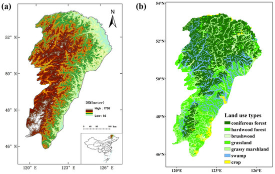
Figure 1.
DEM data in 2013 (a) and land use type in 2020 (b).
2.2. Data Source
2.2.1. Vegetation Data
The GIMMS dataset [53] compiled NDVI images acquired by AVHRR sensors on NOAA satellites. The database consists of quasi-15-day composite data from July 1981. The equatorial data have a spatial resolution of 8 km. More than 22 years of data are covered by the following five different satellites: NOAA-7, -9, -11, -14, and -16. NDVI images were obtained from AVHRR channel 1 and 2 images, which correspond, respectively, to red (0.58–0.68 μm) and near infra-red wavelengths (0.73–1.1 μm). The validity of the GIMMS dataset has been discussed in previous studies [54,55], so we used the product directly here.
The GIMMS3g NDVI data were obtained from NASA Earth Exchange. In order to only analyze the years with complete data coverage, the GIMMS NDVI products used in this paper are from January 1982 to December 2015. Due to part of the pre-processing work of this product has been completed by NASA, the data pre-processing process in this paper included the conversion of data format from nc to tiff and the consistency of projection. Then, the data corresponding to the spatial scope of the research area were extracted. The projection coordinate of this dataset adopted WGS_1984_UTM_Zone_51N. To further reduce the impact of cloud pollution, the bi-monthly data were summarized as monthly composite data by maximum value composite method (MVC) [56].
In this study, all pixel values with NDVI > 0.1 (those with NDVI less than 0.1 were regarded as no vegetation) were first averaged. And we obtained a time series D(t) with 408 values (1982–2015, with an interval of one month). D(t) was used as the original value to explore the overall vegetation change in the study area. On this basis, pixel-by-pixel processing in space was carried out to explore the time series change in each pixel.
2.2.2. Climate Data and Other Geospatial Auxiliary Data
The precipitation (pre) and temperature (tem) dataset in this paper adopted the Chinese Ground Precipitation and temperature 0.5° × 0.5° Gridded Dataset (V2.0) from China Meteorological Data Network (http://data.cma.cn/ (accessed on 22 April 2021)). The dataset is based on monthly precipitation and temperature data of 2472 national stations from 1981 to 2015. The data comes from the information data of Monthly Surface Meteorological Records reported by the climatic data processing departments of all provinces, municipalities, and autonomous regions. The basic data are specially collected and collated by the National Meteorological Information Center and have gone through strict inspection and verification. In order to eliminate the influence of elevation on the spatial interpolation accuracy of precipitation and temperature under the unique terrain conditions in China, GTOP030 data were used to resample the 0.50 × 0.50 DEM in China. Thin plate smoothing spines (TPS) from the ANUSPLIN software for spatial interpolation were used in order to eliminate the elevation factor from the results as much as possible. Monthly data files from January 1982 to December 2015 are used in this paper; additionally, the units of precipitation and temperature are °C and mm, respectively. Climate data were preprocessed, including mosaic, clipping, projection transformation, and resample, which had the same spatial resolution as the GIMMS data. Then, the temporal variation characteristics of precipitation and temperature and their effects on vegetation change were analyzed.
DEM, as digital elevation model, is important original data for studying and analyzing terrain, watershed, and ground object recognition. Digital elevation model data were constructed by linear and bilinear interpolation on the basis of TIN algorithm is provided by geographic monitoring cloud platform (http://www.dsac.cn/ (accessed on 15 November 2020)); additionally, its resolution is 30 m. In this paper, we used the ARCGIS software (https://www.arcgis.com/index.html (accessed on 15 July 2023))to simply transform projection and cut the downloaded elevation data to obtain the elevation data of the whole research area.
Land use data products are Landsat TM/ETM/OLI remote sensing images as the main data source. After image fusion, geometric correction, image enhancement, and mosaic processing, the land use types are divided into 6 first-level classes, 25 second-level classes, and some third-level classification land use data products through human–computer interaction and visual interpretation. In this study, the data were reclassified into five categories, namely, woodland, cultivated land, grassland, water area, and others, so as to better understand the land use types in the study area.
3. Methods
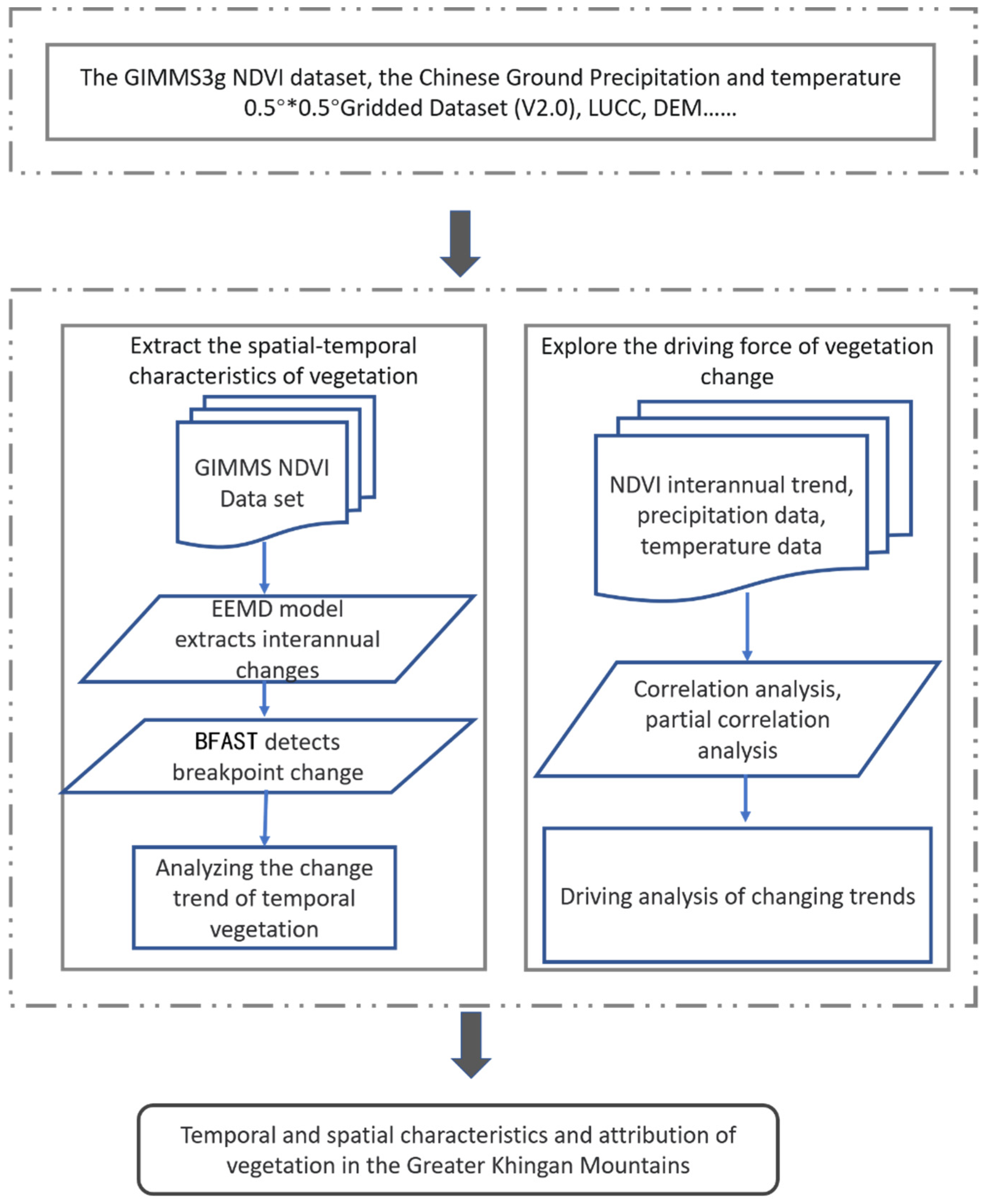
The vegetation change trend detection was based on the time series data analysis. The EEMD was applied first to detect the evolution and change in vegetation spatial and temporal patterns, then BFAST method was used to deal with the interannual variation trend to obtain the variation trend and mutation point, the law of vegetation variation was further explored. As for the key driving factors of spatio-temporal evolution of vegetation trend, correlation analysis was applied to explore the impact of precipitation and temperature on vegetation change, the mechanism of vegetation change was also explored. The flowchart of the study is shown in Figure 2.
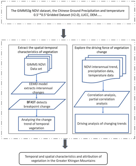
Figure 2.
Flowchart of the study.
3.1. Ensemble Empirical Mode Decomposition (EEMD)
Ensemble empirical mode decomposition (EEMD) is a signal analysis method that is suitable for analyzing nonlinear and non-stationary time series created by Huang et al. [43]. It decomposes complex data into a finite number of oscillating components at different time scales. This decomposition is based on the data themselves without introducing basis functions in advance. Its essence is that the time spectrum is obtained by Hilbert transform after local stabilization of data and is developed on the basis of empirical mode decomposition (EMD).
The method makes use of the principle of taking the average of multiple measurements, and adds appropriate white noise into the original data to simulate the scene of multiple observations, and then makes the ensemble average after multiple calculations. That is, on the basis of empirical mode decomposition, one or more groups of white noise signals are added to suppress the phenomenon of mode mixing in the process of EMD so that the decomposed components maintain the uniqueness of physical properties.
The calculation formula of EMD is as follows:
where represents original data, represents several decomposed components, which has a corresponding average period , and represents residual. The EEMD method iteratively adds Gaussian white noise to the input data to decompose . Specific details of the EEMD algorithm implementation and parameters are provided by Huang et al. [43].
In this paper, the method is used to decompose the long time series of vegetation and climate on multiple time scales, and extract the interannual and long-term change trends of vegetation and climate.
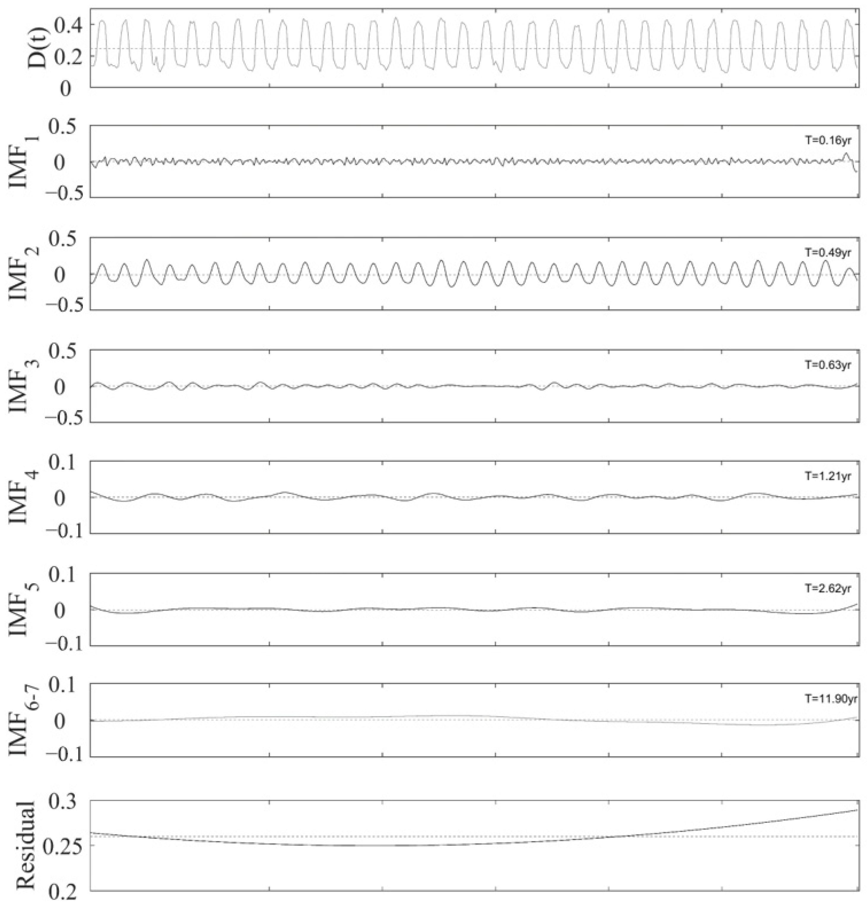
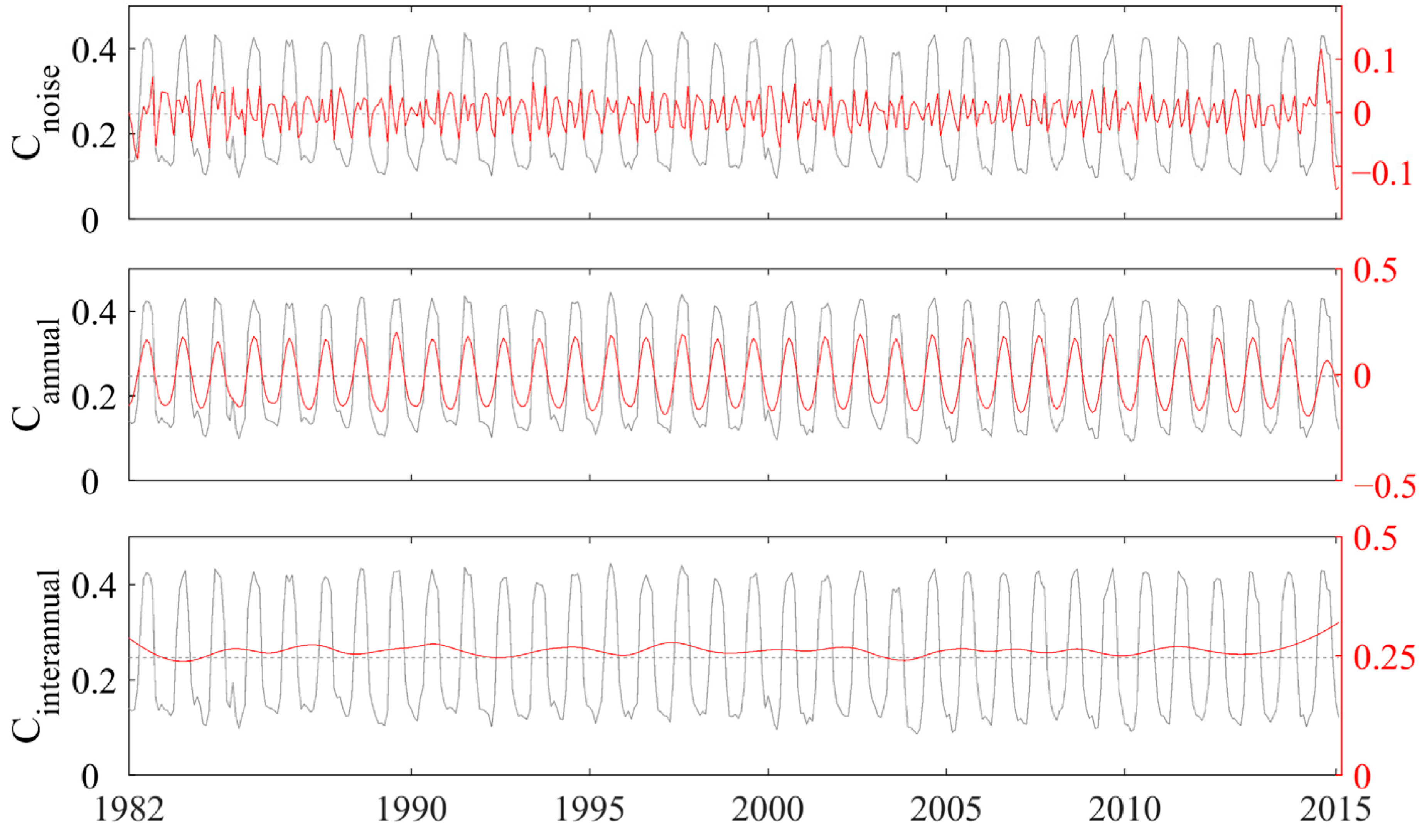
According to the Formula (1), time series NDVI data were decomposed into n components and a residual, as shown in Figure 3. Each had its average period calculated by dividing the number of maxima by the number of years (34). In this study, with was classified as noise component, with was classified as seasonal component, and with and residual was classified as interannual component. The based on the cycle are grouped into noise trends (), seasonal trends (), and interannual trends (), respectively (as shown in Figure 4). Finally, the interannual variation trend of regional scale NDVI time series was extracted.
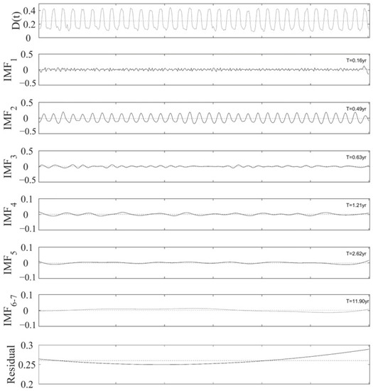
Figure 3.
IMF components and residuals extracted from EEMD.
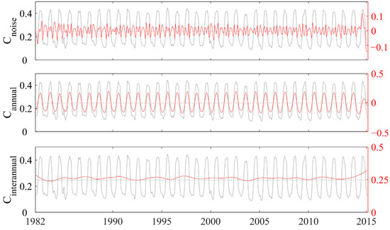
Figure 4.
Noise (), annual () and interannual trend () at the regional scale.
3.2. Breaks for Additional Seasonal and Trend (BFAST)
Time series breakpoint recognition algorithm BFAST is a time series change detection model proposed by Verbesselt et al. [52]. It is a repeated iterative change diagnosis method. It judges whether there are breakpoints and determine the number and location of breakpoints [10]. It has the advantages of it not being necessary to set threshold, no need to define change trajectory, and can eliminate noise interference. The algorithm form of the model is as follows:
where, is the value observed at time ; is trend component; is seasonal component; is the residual; that is, the variation beyond seasonality and trend. In this paper, the seasonal component is zero.
3.3. Relationship Analysis Methods
The correlation coefficient can be used to express the correlation degree of two groups of variables, and the correlation between NDVI data and climate parameters in the Greater Khingan Mountains is analyzed by this coefficient. Partial correlation analysis can ignore the influence of other factors when studying the relationship between factors, so this method is used to explore the independent correlation between NDVI data and a single climate parameter.
3.4. Correlation Analysis
Correlation analysis can measure the relationship between elements. In this study, correlation analysis was used to analyze the response degree of NDVI to meteorological elements. The mathematical expression of correlation analysis is the following:
where, is the research duration; represents precipitation or temperature at the th time point; and represents the average value of precipitation or temperature during the study period. represents the vegetation status at the th time point and represents the mean value of vegetation status during the study period.
3.5. Partial Correlation Analysis
Natural system is a complex system with many elements, especially in the natural system composed of many elements, the change in one element will inevitably affect the change in other elements. When studying the influence or correlation degree of one element on another element, partial correlation regards the influence of other elements as a constant (unchanged). The statistics used to measure the degree of partial correlation become the partial correlation coefficient. The specific formula is as follows:
where, represent the partial correlation coefficient between factor and factor after factor is fixed; , , and represent the correlation coefficients of factor and factor , factor and factor , and factor and factor , respectively.
4. Result
4.1. Temporal Variation Characteristics of NDVI
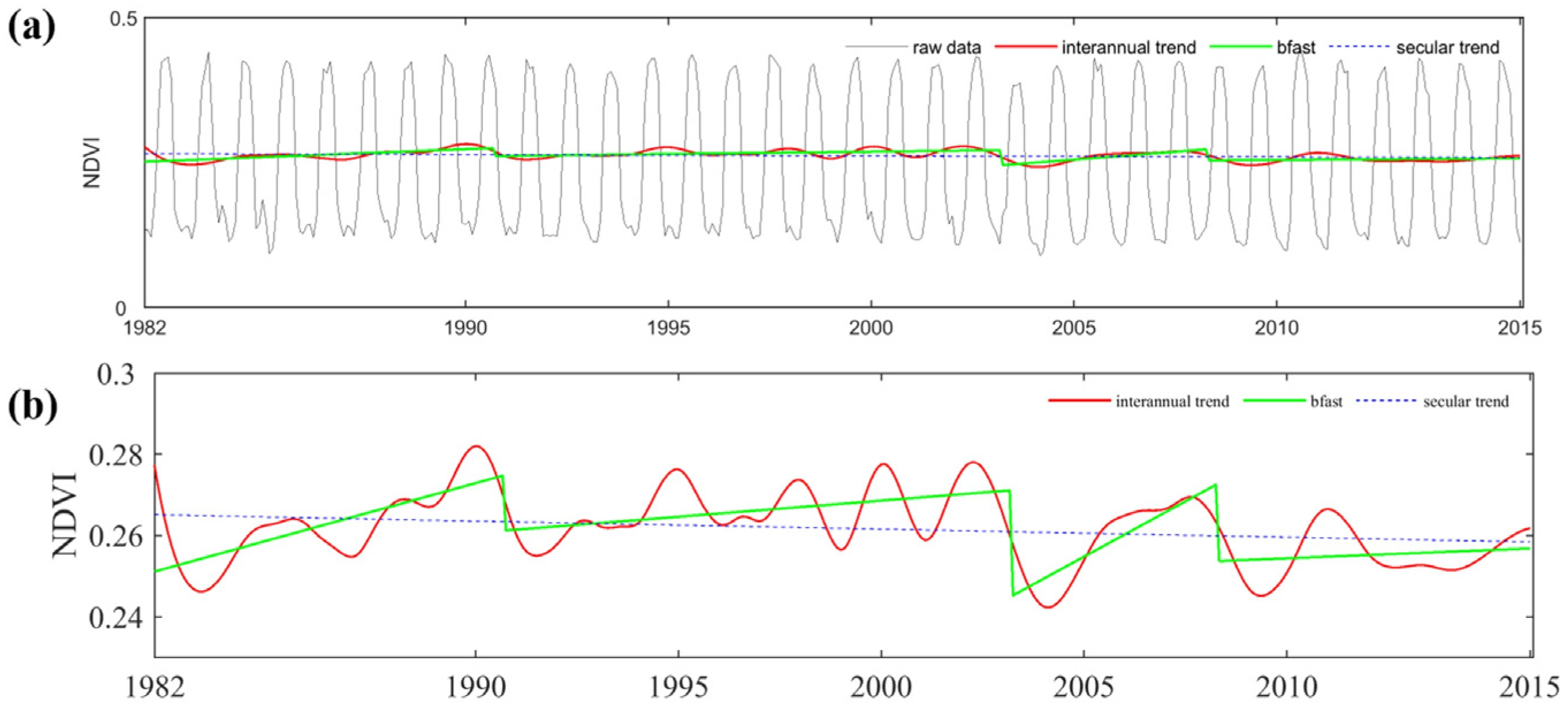
The interannual variation of NDVI in the whole study area is shown in Figure 5. As can be seen from the figure, the original data had obvious seasonal characteristics and noise (Figure 5a). After extracting vegetation trends using the EEMD method, the NDVI changes had significant fluctuations (as shown by the solid red line in Figure 5b) and showed a decreasing trend (as shown by the dotted blue line in Figure 5b, slope = −0.1645/10,000, p < 0.01) in the whole time series. At the same time, according to the formula of BFAST in Section 3.2, we also detected three breakpoint changes, which were in 1990, 2003, and 2008, respectively. During 1982–1990 and 2003–2008, NDVI showed a trend of sharp increase (the slope was 0.0023/10,000 and 0.0045/10,000, p < 0.01), while in the other two periods, NDVI showed a relatively weak positive trend (Figure 5b, slopes were 0.0007/10,000 and 0.0003/10,000, p < 0.01). The interannual trend obtained by the EEMD method can obtain the changes of vegetation in the whole time series in more detail. In addition, BFAST can detect breakpoints, and short-term changes can be better captured by taking breakpoints as short-term detection time points.
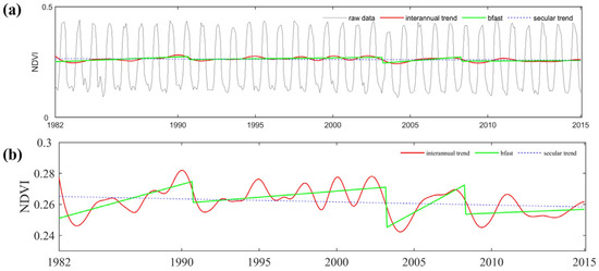
Figure 5.
Secular trend, interannual trends, and mutation at regional scales (a,b).
4.2. Spatial Variation of NDVI
4.2.1. The Interannual Variation Trend of NDVI
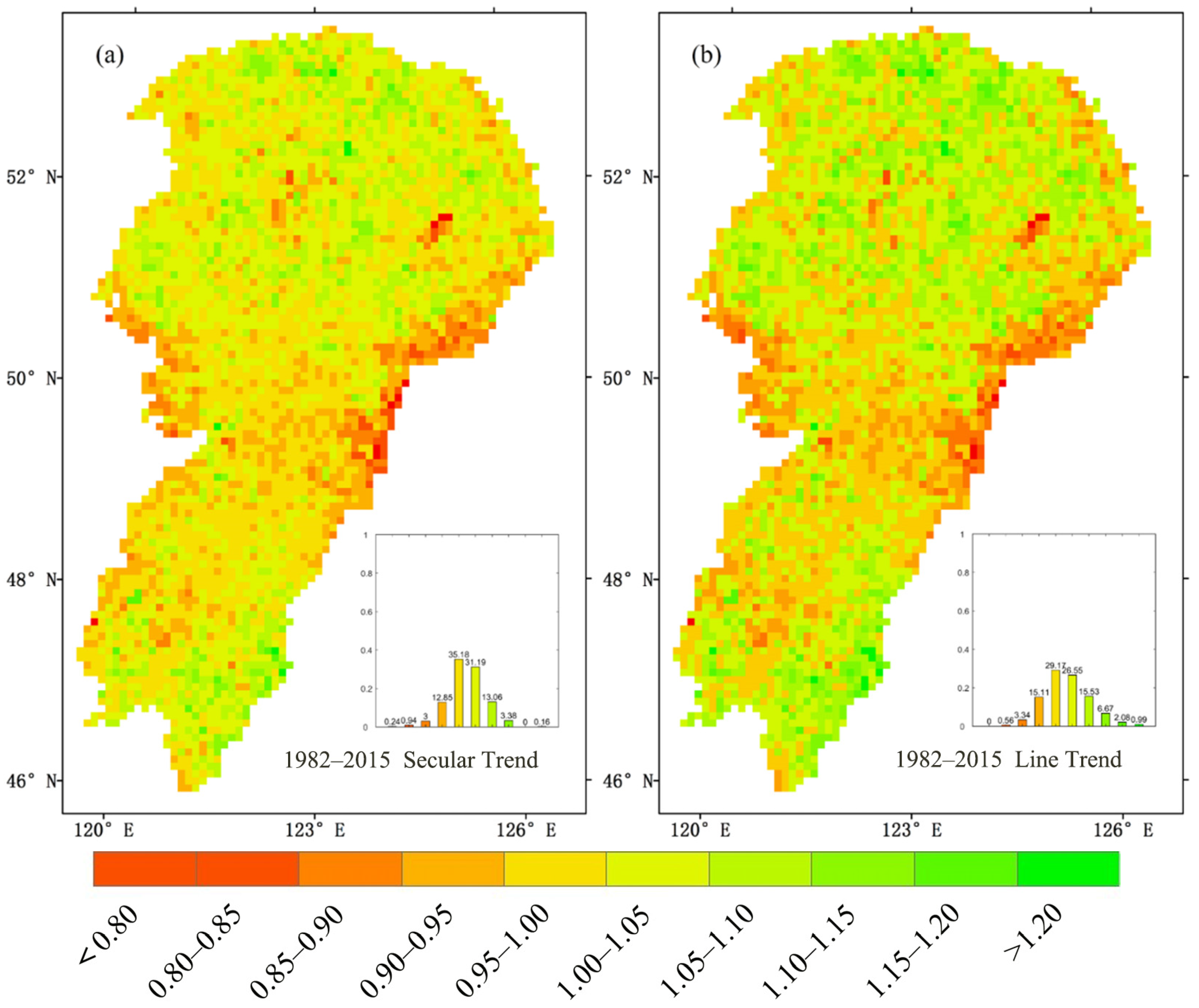
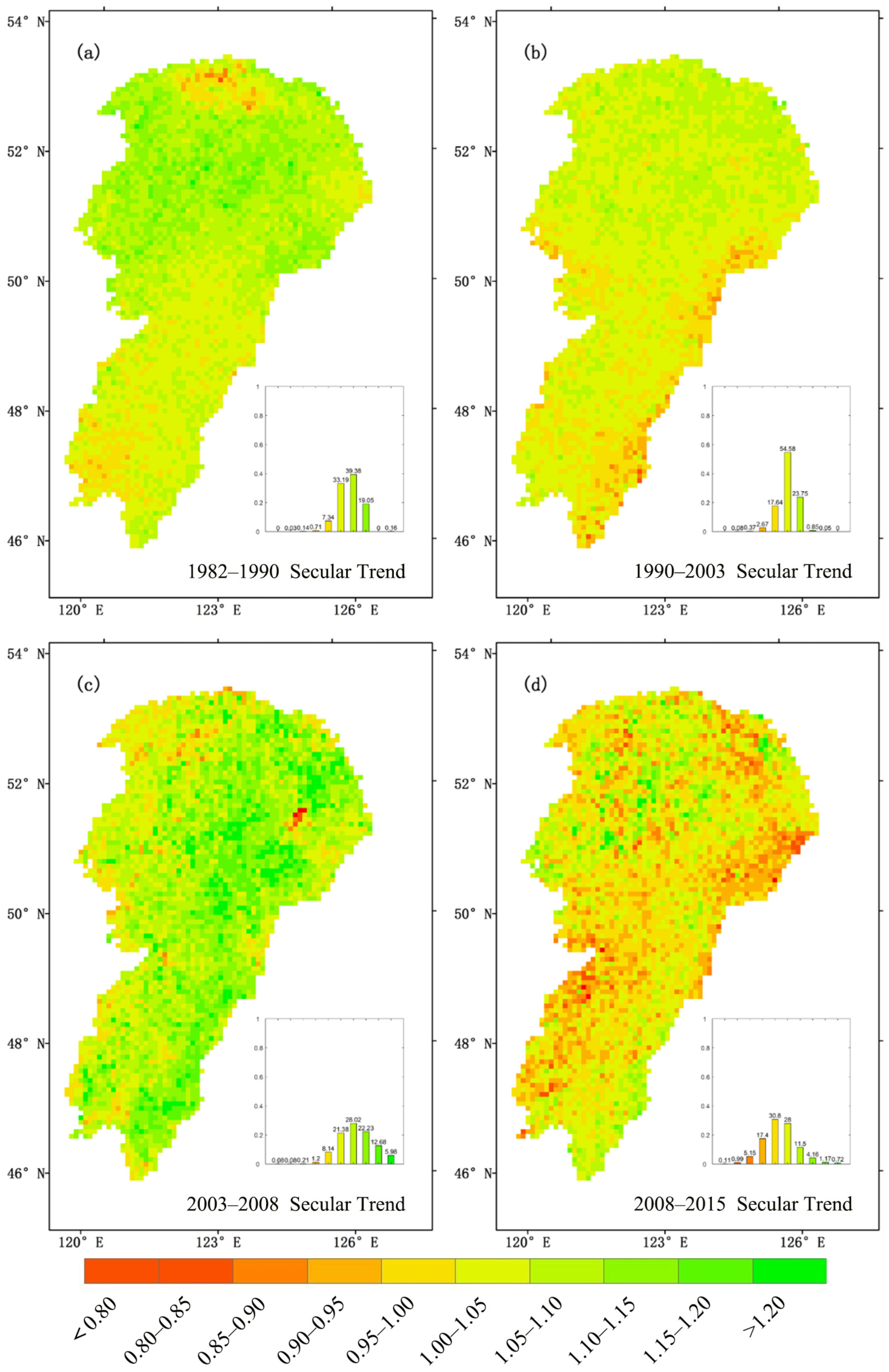
Secular trends, which represent the cumulative trend from the start time to a given time, are the natural trends extracted by EEMD and can detect more subtle changes than linear trends. In this study, we started the long-term trend in 1982 and ended it with the breakpoints (1990, 2003, 2008) and the last year (2015). To avoid the problem of too small and concentrated data, we represented the change as the difference degree (NDVI ratio of the end time and the start time) instead of the difference. When the value was greater than one, it indicated the greening trend of vegetation; therefore, when the value was less than one, it indicated the browning trend of vegetation. The spatio-temporal variation of NDVI in the whole time period is shown in Figure 6. From the 1980s to the 1990s, more than 90% of the vegetation in the study area showed a greening trend. The greening degree in most areas (70.96%) increased about 10% compared with 1982, and the greening degree in the upper middle area increased by 10%–20% compared with 1982. Only about 8% of the area showed browning, and most of them are in the north and southwest of the study area (Figure 6a). By 2003, the degree of vegetation greening and browning was mainly concentrated in the range of 10%, accounting for 84.97% and 12.94%, respectively. And the browning area was concentrated in the eastern and western area (Figure 6b). By 2008, about 30% of the area showed a browning trend, in which about 7% of the area showed a browning trend with a browning degree more than 5%. By 2015, the greening and browning areas accounted for almost half, respectively, while the browning area was slightly larger than that of greening. The browning area gradually expanded from the marginal part to the central region. As shown in Figure 7, the vegetation change characteristics extracted by the EEMD and linear methods in the Greater Khingan Mountains from 1982 to 2015 was similar, but the change degree extracted by the linear method was stronger than that of EEMD, indicating that the linear method makes the change more significant.
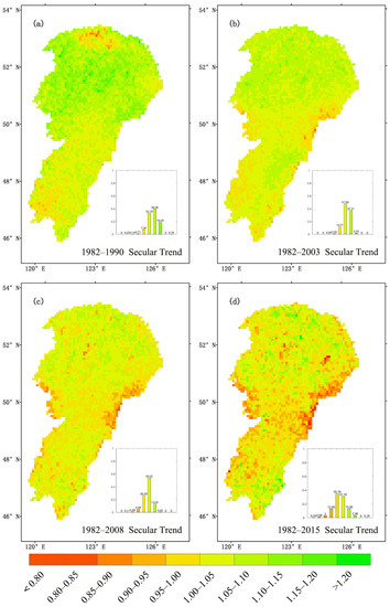
Figure 6.
Temporal and spatial nonlinear variation of NDVI. Spatial distribution of the four times evolutions during (a) 1982–1990, (b) 1982–2003, (c) 1982–2008, and (d) 1982–2015. The histogram represents the pixel ratio of different NDVI change levels in the whole study area.

Figure 7.
Secular trend change trend of NDVI from 1982 to 2015. (a) Change in NDVI extracted by EEMD, (b) change in NDVI extracted by linear method. The histogram represents the pixel ratio of different NDVI change levels in the whole study area.
4.2.2. Variation Trend of NDVI in Different Time Periods
In order to explore the hidden change characteristics of NDVI in the whole time series, we studied the nonlinear and linear changes of vegetation in 1982–1990, 1990–2003, 2008–2008, and 2008–2015 by taking the breakpoint as the boundary. The results indicate that in the period of 1982–1990, 1990–2003, and 2003–2008, most of the area indicated a greening trend with an area percent of 92%, 80%, and 90%, respectively, and a browning trend was detected in 2008–2015, with 54.45% of the area showing a NDVI decreasing (Figure 8). This result is consistent with the vegetation change in the whole study area in Figure 5. Similar to the spatial distribution of secular trends (Figure 6), a browning trend often occurred in marginal areas first, and when the browning occurred in a certain area in the current period, the vegetation in the latter period usually showed a certain degree of restoration. For example, in the northern area, a browning trend was detected in 1982–1990 (Figure 8a), a corresponding greening trend was found in this area in 1990–2003 (Figure 8b).

Figure 8.
Spatial distribution of short-term changes in NDVI. NDVI short-term nonlinear change spatial distribution maps for (a) 1982–1990, (b) 1990–2003, (c) 2003–2008, and (d) 2008–2015. The histogram represents the pixel ratio of different NDVI change levels in the whole study area.
4.3. Response of NDVI to Climatic Drivers
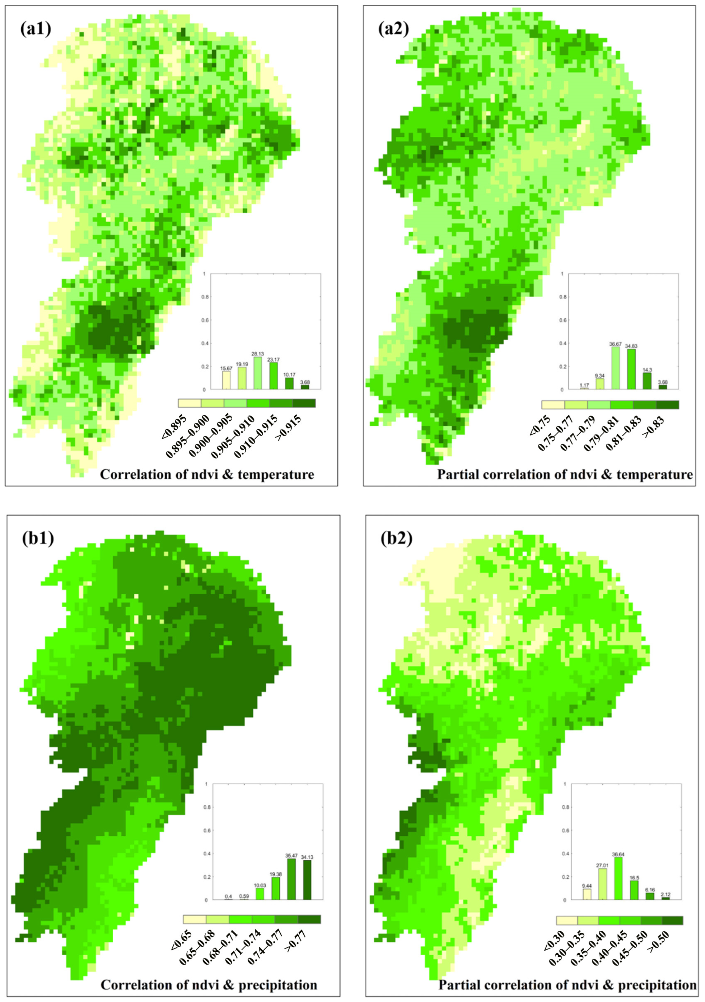
In order to explore the driving mechanism of vegetation change, Figure 9 shows the correlation and partial correlation between vegetation and climatic conditions (temperature, precipitation) according to the formula (3) and formula (4) in Section 3.3. In general, there is a significant positive correlation between NDVI and precipitation and temperature in the Greater Khingan Mountains (p < 0.05), and the correlation between NDVI and temperature is always greater than that of precipitation, indicating that temperature has a greater impact on vegetation than precipitation. Compared with the results of the correlation analysis, the value of the partial correlation analysis is relatively small, which indicates that other factors do affect the results in the correlation analysis between single factor and vegetation.

Figure 9.
Correlation between vegetation change and climate factors. (a1) Correlation between NDVI change and temperature. (a2) Partial correlation between NDVI change and temperature. (b1) Correlation between NDVI change and precipitation. (b2) Partial correlation between NDVI change and precipitation. The histogram represents the pixel ratio of different correlation coefficients levels in the whole study area.
The results showed that the influence degree of climatic conditions on vegetation varies spatially. The correlation between vegetation and temperature is weak in the east and west edges, especially in the low-lying area, while the correlation between vegetation and precipitation is strong. In the southeast area, the correlation between vegetation and temperature is stronger than that of other regions, and the correlation between vegetation and precipitation is weaker than that of other regions.
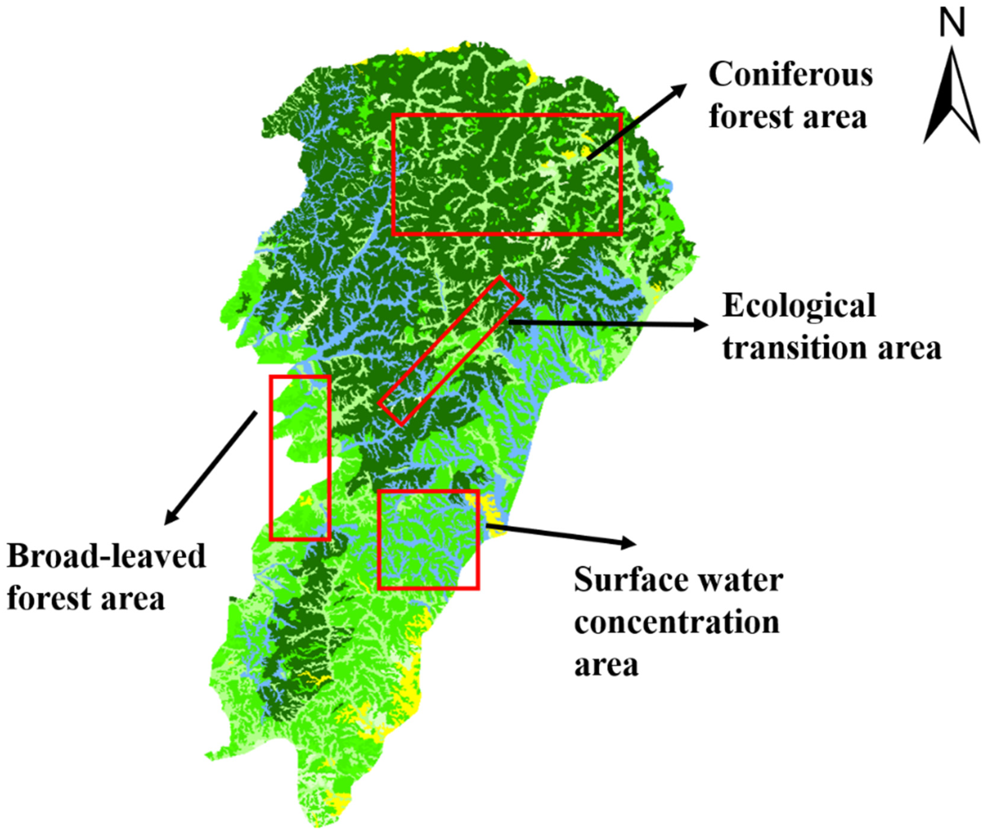
In order to analyze the relationship between vegetation change and climate factors in the Greater Khingan Mountains in detail, we selected four typical ecological regions in the study area. From north to south, the typical ecological areas are the coniferous forest area, the ecological transition area, the broad-leaved forest area, and the surface water concentration area (Figure 10).

Figure 10.
Spatial distribution map of typical study area.
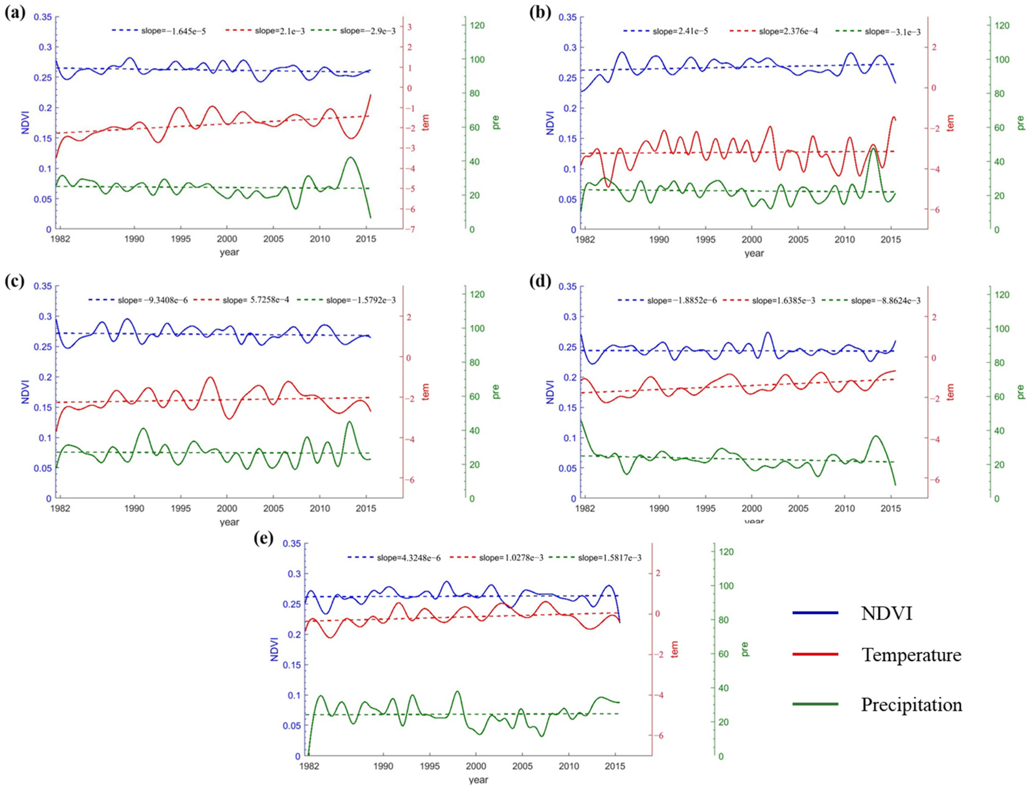
Figure 11 showed the nonlinear changes of temporal NDVI and climatic factors (temperature and precipitation) in the whole study area and the four typical ecological regions. The results showed that the temporal NDVI of the study area, the ecological transition area, and the broad-leaved forest area showed a downward trend, while the temporal NDVI of the coniferous forest area and the surface water concentration area showed an upward trend. In the ecological transition area, the NDVI browning trend was the largest, with a slope of , while in the coniferous forest area, The NDVI greening trend was the largest, with a slope of . Temperature in the four regions showed an increasing trend, among which the broad-leaved forest area showed the largest increasing trend, with a slope of . Except for the surface water concentration area, the precipitation showed a decreasing trend in the typical ecological area. And the precipitation in the broad-leaved forest area showed the largest decreasing trend, with a slope of .
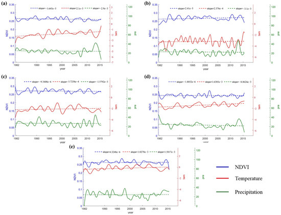
Figure 11.
Nonlinear changes of temporal NDVI and climate factors during 1982–2015: (a) the Greater Khingan Mountains Research Area, (b) the coniferous forest area, (c) the ecological transition area, (d) the broad-leaved forest area, and (e) the surface water concentration area.
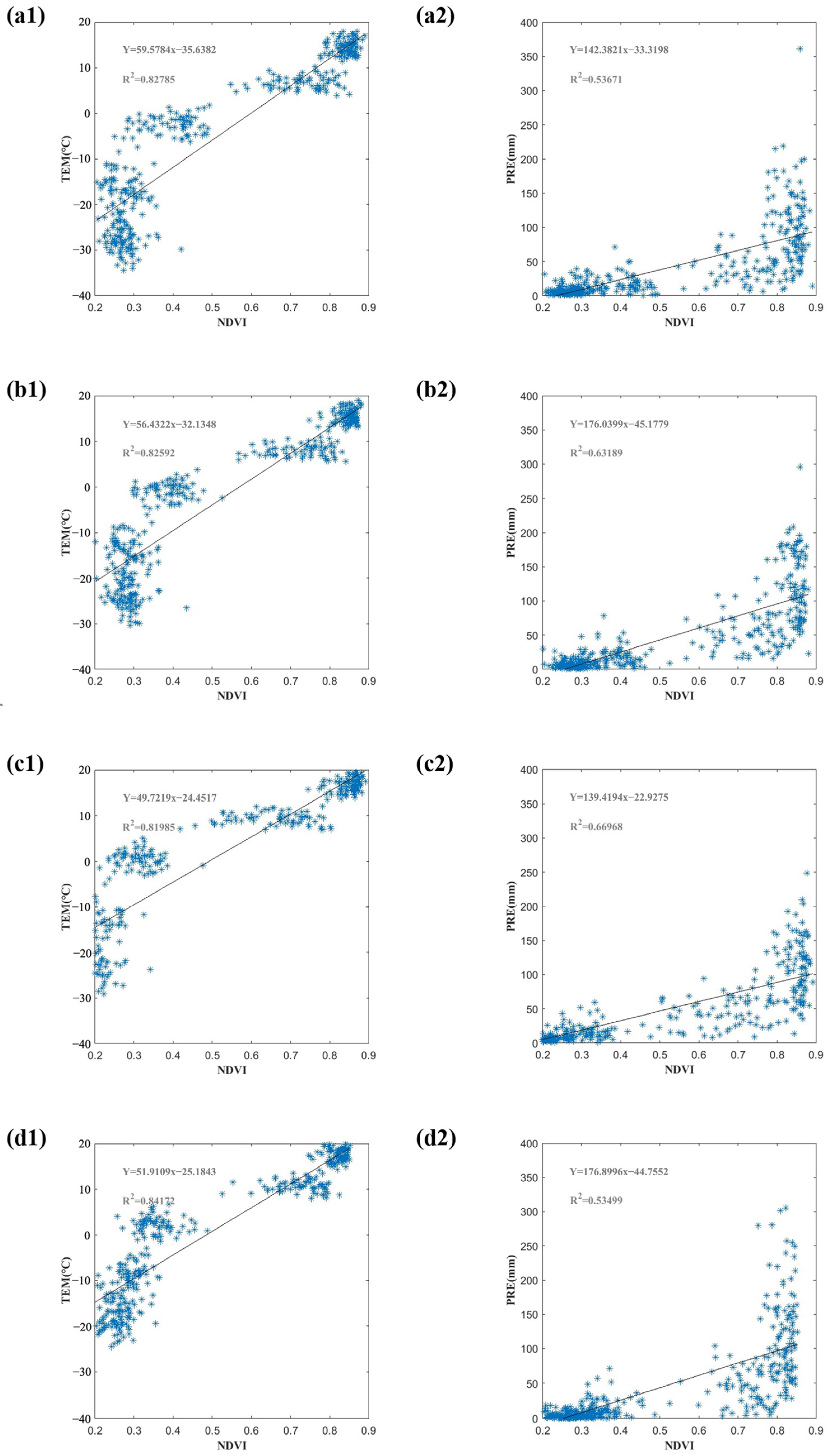
Figure 12 showed the relationship between temporal NDVI and climatic factors (temperature and precipitation) in the four typical ecological regions. In the four typical ecological regions, the correlation coefficient between NDVI and temperature is greater than 0.8, and the correlation coefficient between NDVI and precipitation is greater than 0.5.
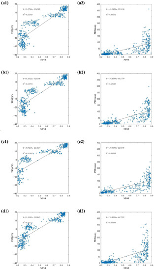
Figure 12.
Scatter plots of NDVI and climatic factors in four typical ecological regions during 1982–2015. (a1,a2) Coniferous forest area, (b1,b2) ecological transition area, (c1,c2) broad-leaved forest area, and (d1,d2) surface water concentration area.
In the surface water concentration area, the correlation coefficient between NDVI and temperature was the largest, reaching 0.842. While the correlation coefficient between NDVI and precipitation was the smallest, reaching 0.535. The above-ground water resources in this region provide sufficient water for vegetation growth, so vegetation growth is less affected by precipitation and more affected by temperature.
In the broad-leaved forest area, the correlation coefficient between NDVI and air temperature was the smallest, reaching 0.820. While the correlation coefficient between NDVI and precipitation was the largest, reaching 0.670. This region is located at the edge of the study area, where strong solar radiation and wind speed make vegetation growth less affected by temperature, but more dependent on precipitation.
5. Discussion
5.1. Compare with Previous Studies
In this research, the NDVI change in vegetation in the Greater Khingan Mountains from 1982 to 2015 was declining, which is consistent with the study of Mao et al. [57], but different from the results of Hu et al. [29]. The reason for the difference may be that the scope of the study area is slightly different. For example, the study area of Hu et al. only included the Greater Khingan Mountains in Heilongjiang Province. While from a spatial perspective, the results of Hu et al.’s research were consistent with the conclusions of this paper, indicating that vegetation in the northern part of the Greater Khingan Mountains has a certain degree of greening.
The BFAST method was used to detect three obvious breakpoints in 1990, 2003, and 2008 in the Greater Khingan Mountains. Peng et al. showed that the increase in NDVI in the growing season in northern China during 1982–1990s was attributed to the warming trend and more precipitation, while the drought caused by warming and decreased precipitation resulted in the decrease in NDVI in the growing season after 1990s or early 2000s [58]. The apparent browning of vegetation in 1990 may be related to the dual effects of precipitation and major fires in 1987 [59]. He et al. showed that in recent years, the drought in the Greater Khingan Mountains study area was serious, which would lead to vegetation browning, vegetation mortality changes, and even ecosystem degradation [60]. The abrupt changes in vegetation in 2003 and 2008 were due to high temperatures and droughts caused by reduced precipitation. Although the correlation between temperature and NDVI dynamics is more significant, the change in NDVI may be greatly regulated by precipitation [61].
The vegetation change was positively correlated with temperature and precipitation, and the correlation with temperature was higher. This conclusion is consistent with the results of Yang et al. [62]. The east and west edges of the study area are forest boundaries. Due to the complexity of land types and the enhancement of human activities (especially farmland), this area has a strong degree of fragmentation. The forest margins may be more vulnerable to drought; therefore, the region is more dependent on precipitation. According to the Chinese ecological geographic zoning map [63], the middle part is just the dividing line between the broad-leaved forest area and the coniferous forest area. In this area, vegetation goes not grow very well, which results the more exposure of land and further causes an increase in wind speed and radiation intensity; therefore, the influence of precipitation is greater than that of other regions. In the southeast area, which is located in the hilly areas of the Greater Khingan Mountains, the above-ground water resources provide sufficient water for vegetation growth [59]; thus, vegetation change was relatively less affected by precipitation.
5.2. Data Selection and Parameter Setting
As for the selection of data, AVHRR NDVI and MODIS NDVI are the NDVI data commonly used by researchers to explore the temporal and spatial variation characteristics of vegetation. In this study, we compared the differences between the two products. In the Greater Khingan Mountains research area, although the value of GIMMS NDVI is larger than that of MODIS NDVI, and the variation trend of the two is slightly different, the variation trend of GIMMS NDVI and MODIS NDVI are basically the same within the overlapping time range, so we chose GIMMS NDVI with a wider temporal coverage in this study. Meanwhile, in order to further eliminate the influence of noise, we processed the monthly maximum value of GIMMS NDVI data. Although remote sensing data can obtain large range and long time series vegetation data, noise data will inevitably be mixed into NDVI data due to various reasons, such as sensor offset, cloud and fog influence, data splicing, algorithm inversion, and so on, which further lead to deviation in vegetation trend analysis. At the same time, fire and flood also cause sudden changes in a short time, so linear changes cannot be simply considered.
In this study, we discussed the evolution characteristics of vegetation by combining long-term trend and mutation. Among them, the EEMD method has all the advantages of EMD. Different from EMD, two parameters need to be set when EEMD is used, namely, the amplitude coefficient k of the white noise sequence added to the signal and the total number M of EMD performed by the algorithm. The smaller the k is, the better it can improve the decomposition accuracy; however, when k is small to a certain degree, it may not be sensitive enough to detect the local extreme point. The other parameter is M; the larger the M is, the smaller the impact of noise on decomposition is and the heavier computational burden is. Therefore, in this study, we analyze the values of these two parameters, and find that when the k value is 0.2–0.4 and the M value is larger than 100, the white noise has little influence on the decomposition results; therefore, in this study, k is set to be 0.2 and M is 100. The error induced by the parameter setting is considered acceptable.
5.3. Other Factors in Correlation Analysis
The vegetation index is affected by many factors, such as natural and human activities. As a well-preserved original forest region in China, the greater Khingan Mountains forest is less affected by human activities [64]. Therefore, we did not consider the impact of human activities on vegetation change in this study, but this does not mean that human activities have no effect on this region. The policy of returning farmland to forest increases the area of forest in China, but in this study, the area of forest was fixed. At the same time, other factors in the natural environment will also affect vegetation change. For example, different terrain will not only affect remote sensing data acquisition, but also affect vegetation change [65]; furthermore, the distribution structure of vegetation itself also has a certain impact on vegetation change [66]. Li et al. used the geodetector method to analyze the influence of 15 natural factors and human factors on vegetation change, and the results show that the q statistics of all influencing factors passed the significance test [34]. Natural factors include soil type, precipitation, air temperature, wind speed, radiation, and so on; therefore, the influence of natural environment on vegetation is relatively complex. In the analysis, not only the effect of single factor on vegetation change should be studied, but also the joint effect of each factor on vegetation change should be considered.
6. Conclusions
In this paper, nonlinear and non-stationary EEMD and BFAST breakpoint (abrupt change) methods were used to investigate the temporal and spatial evolution characteristics of the vegetation in the Greater Khingan Mountains from 1982 to 2015. The relationship between the vegetation and climatic factors is further quantified. The results show that from 1982 to 2015, there was no obvious trend of vegetation browning in the whole study area. An obvious browning trend was found on the east and west sides of the forest where severe marginalization exists. When using the breakpoint method to capture the mutation point, we found that the browning degree of vegetation was obvious in 1990, 2003, and 2008, and there was a certain greening trend after the mutation point. Vegetation change had obvious spatial characteristics. From 1982 to 2015, about 50% of the area showed browning characteristics, and the browning area expanded from the edge to the center area.
In addition, we used the correlation analysis and partial correlation analysis methods to explore the relationship between climate factors and vegetation. The result shows that the vegetation and climate factors (precipitation, temperature) in the Greater Khingan Mountains study area showed an obvious positive correlation. The change in NDVI has a strong correlation with temperature, with a correlation coefficient range of [0.8–1]. At the same time, the difference between the partial correlation analysis and the correlation analysis results indicates that the relationship between various climatic factors and vegetation is not independent, but mutual influence.
Author Contributions
Conceptualization, methodology, software, project administration, funding acquisition, validation, writing—review and editing, H.Z.; formal analysis, software, validation, visualization, writing—original draft preparation, W.F.; software, validation, W.M., Q.W. and W.F., C.W. and G.Z. All authors have read and agreed to the published version of the manuscript.
Funding
This research was funded by the National Natural Science Foundation of China grant number 42171313, 42090012.
Institutional Review Board Statement
Not applicable.
Informed Consent Statement
Not applicable.
Data Availability Statement
The GIMMS3g NDVI data were obtained on the NASA Earth Exchange (https://ecocast.arc.nasa.gov/data/pub/gimms/, accessed on 13 November 2020). The precipitation (pre) and temperature (tem) dataset adopted the Chinese Ground Precipitation and temperature 0.5° × 0.5°Gridded Dataset (V2.0) from China Meteorological Data Network (http://data.cma.cn/, accessed on 22 April 2021). Land use data products and digital elevation model were available on the geographic monitoring cloud platform (http://www.dsac.cn/, accessed on 13 November 2020).
Conflicts of Interest
The authors declare no conflict of interest.
References
- Chen, J.; Yan, F.; Lu, Q. Spatiotemporal variation of vegetation on the Qinghai–Tibet Plateau and the influence of climatic factors and human activities on vegetation trend (2000–2019). Remote Sens. 2020, 12, 3150. [Google Scholar] [CrossRef]
- Tang, L.; He, M.Z.; Li, X.R. Verification of Fractional Vegetation Coverage and NDVI of Desert Vegetation via UAVRS Technology. Remote Sens. 2020, 12, 1742. [Google Scholar] [CrossRef]
- Xu, R.; Li, Y.; Teuling, A.J.; Zhao, L.; Spracklen, D.V.; Garcia-Carreras, L.; Meier, R.; Chen, L.; Zheng, Y.T.; Lin, H.Q.; et al. Contrasting impacts of forests on cloud cover based on satellite observations. Nat. Commun. 2022, 13, 670. [Google Scholar] [CrossRef] [PubMed]
- De Jong, R.; Verbesselt, J.; Schaepman, M.E.; De Bruin, S. Trend changes in global greening and browning: Contribution of short-term trends to longer-term change. Glob. Chang. Biol. 2012, 18, 642–655. [Google Scholar] [CrossRef]
- Abbas, S.; Nichol, J.E.; Wong, M.S. Trends in vegetation productivity related to climate change in China’s Pearl River Delta. PLoS ONE 2021, 16, e0245467. [Google Scholar] [CrossRef]
- Feng, Y.; Zeng, Z.Z.; Searchinger, T.D.; Ziegler, A.D.; Wu, J.; Wang, D.S.; He, X.Y.; Elsen, P.R.; Ciais, P.; Xu, R.R.; et al. Doubling of annual forest carbon loss over the tropics during the early twenty-first century. Nat. Sustain. 2022, 5, 444–451. [Google Scholar] [CrossRef]
- Osland, M.J.; Hughes, A.R.; Armitage, A.R.; Scyphers, S.B.; Cebrian, J.; Swinea, S.H.; Shepard, C.C.; Allen, M.S.; Feher, L.C.; Nelson, J.A.; et al. The impacts of mangrove range expansion on wetland ecosystem services in the southeastern United States: Current understanding, knowledge gaps, and emerging research needs. Glob. Chang. Biol. 2022, 28, 3163–3187. [Google Scholar] [CrossRef]
- Zhu, Z.C.; Piao, S.L.; Myneni, R.B.; Huang, M.T.; Zeng, Z.Z.; Canadell, J.G.; Ciais, P.; Sitch, S.; Friedlingstein, P.; Arneth, A.; et al. Greening of the Earth and its drivers. Nat. Clim. Chang. 2016, 6, 791–795. [Google Scholar] [CrossRef]
- Piao, S.L.; Fang, J.Y.; Ciais, P.; Peylin, P.; Huang, Y.; Sitch, S.; Wang, T. The carbon balance of terrestrial ecosystems in China. Nature 2009, 458, 1009–1082. [Google Scholar] [CrossRef]
- Pettorelli, N.; Vik, J.O.; Mysterud, A.; Gaillard, J.M.; Tucker, C.J.; Stenseth, N.C. Using the satellite-derived NDVI to assess ecological responses to environmental change. Trends Ecol. Evol. 2005, 20, 503–510. [Google Scholar] [CrossRef]
- Asokan, A.; Anitha, J. Change detection techniques for remote sensing applications: A survey. Earth Sci. Inf. 2019, 12, 143–160. [Google Scholar] [CrossRef]
- Fang, H.L.; Baret, F.; Plummer, S.; Schaepman-Strub, G. An Overview of Global Leaf Area Index (LAI): Methods, Products, Validation, and Applications. Rev. Geophys. 2019, 57, 739–799. [Google Scholar] [CrossRef]
- Chen, J.M.; Cihlar, J. Retrieving leaf area index of boreal conifer forests using landsat TM images. Remote Sens. Environ. 1996, 55, 153–162. [Google Scholar] [CrossRef]
- Zhang, M.; Wang, J.M.; Li, S.J. Tempo-spatial changes and main anthropogenic influence factors of vegetation fractional coverage in a large-scale opencast coal mine area from 1992 to 2015. J. Clean. Prod. 2019, 232, 940–952. [Google Scholar] [CrossRef]
- Chen, Y.Z.; Feng, X.M.; Tian, H.Q.; Wu, X.T.; Gao, Z.; Feng, Y.; Piao, S.L.; Lv, N.; Pan, N.Q.; Fu, B.J. Accelerated increase in vegetation carbon sequestration in China after 2010: A turning point resulting from climate and human interaction. Glob. Chang. Biol. 2021, 27, 5848–5864. [Google Scholar] [CrossRef]
- Collalti, A.; Ibrom, A.; Stockmarr, A.; Cescatti, A.; Alkama, R.; Fernandez-Martinez, M.; Matteucci, G.; Sitch, S.; Friedlingstein, P.; Ciais, P.; et al. Forest production efficiency increases with growth temperature. Nat. Commun. 2020, 11, 5322. [Google Scholar] [CrossRef] [PubMed]
- Clark, D.A.; Brown, S.; Kicklighter, D.W.; Chambers, J.Q.; Thomlinson, J.R.; Ni, J. Measuring net primary production in forests: Concepts and field methods. Ecol. Appl. 2001, 11, 356–370. [Google Scholar] [CrossRef]
- Myneni, R.B.; Keeling, C.D.; Tucker, C.J.; Asrar, G.; Nemani, R.R. Increased plant growth in the northern high latitudes from 1981 to 1991. Nature 1997, 386, 698–702. [Google Scholar] [CrossRef]
- Salim, H.A.; Chen, X.; Gong, J. Analysis of Sudan vegetation dynamics using NOAA-AVHRR NDVI data from 1982–1993. Asian J. Eart. Sci. 2010, 3, 20–34. [Google Scholar]
- Xue, J.R.; Su, B.F. Significant Remote Sensing Vegetation Indices: A Review of Developments and Applications. J. Sens. 2017, 2017, 1353691. [Google Scholar] [CrossRef]
- Townshend, J.R.; Masek, J.G.; Huang, C.Q.; Vermote, E.F.; Gao, F.; Channan, S.; Sexton, J.O.; Feng, M.; Narasimhan, R.; Kim, D.; et al. Global characterization and monitoring of forest cover using Landsat data: Opportunities and challenges. Int. J. Digit. Earth 2012, 5, 373–397. [Google Scholar] [CrossRef]
- Hansen, M.C.; DeFries, R.S. Detecting long-term global forest change using continuous fields of tree-cover maps from 8-km advanced very high resolution radiometer (AVHRR) data for the years 1982–99. Ecosystems 2004, 7, 695–716. [Google Scholar] [CrossRef]
- Telesca, L.; Lasaponara, R. Discriminating dynamical patterns in burned and unburned vegetational covers by using SPOT-VGT NDVI data. Geophys. Res. Lett. 2005, 32, L21401. [Google Scholar] [CrossRef]
- Teferi, E.; Uhlenbrook, S.; Bewket, W. Inter-annual and seasonal trends of vegetation condition in the Upper Blue Nile (Abay) Basin: Dual-scale time series analysis. Earth Syst. Dyn. 2015, 6, 617–636. [Google Scholar] [CrossRef]
- De Beurs, K.M.; Henebry, G.M. A statistical framework for the analysis of long image time series. Int. J. Remote Sens. 2005, 26, 1551–1573. [Google Scholar] [CrossRef]
- Guan, Q.Y.; Yang, L.Q.; Pan, N.H.; Lin, J.K.; Xu, C.Q.; Wang, F.F.; Liu, Z.Y. Greening and Browning of the Hexi Corridor in Northwest China: Spatial Patterns and Responses to Climatic Variability and Anthropogenic Drivers. Remote Sens. 2018, 10, 1270. [Google Scholar] [CrossRef]
- De Jong, R.; de Bruin, S.; de Wit, A.; Schaepman, M.E.; Dent, D.L. Analysis of monotonic greening and browning trends from global NDVI time-series. Remote Sens. Environ. 2011, 115, 692–702. [Google Scholar] [CrossRef]
- Ji, F.; Wu, Z.H.; Huang, J.P.; Chassignet, E.P. Evolution of land surface air temperature trend. Nat. Clim. Chang. 2014, 4, 462–466. [Google Scholar] [CrossRef]
- Hu, L.; Fan, W.; Ren, H.; Liu, S.; Cui, Y.; Zhao, P. Spatiotemporal dynamics in vegetation GPP over the great khingan mountains using GLASS products from 1982 to 2015. Remote Sens. 2018, 10, 488. [Google Scholar] [CrossRef]
- Tang, H.; Li, Z.; Zhu, Z.; Chen, B.; Zhang, B.; Xin, X. Variability and climate change trend in vegetation phenology of recent decades in the Greater Khingan Mountain area, Northeastern China. Remote Sens. 2015, 7, 11914–11932. [Google Scholar] [CrossRef]
- Sun, J.Y.; Wang, X.H.; Chen, A.P.; Ma, Y.C.; Cui, M.D.; Piao, S.L. NDVI indicated characteristics of vegetation cover change in China’s metropolises over the last three decades. Environ. Monit. Assess. 2011, 179, 1–14. [Google Scholar] [CrossRef] [PubMed]
- Tomé, A.; Miranda, P. Piecewise linear fitting and trend changing points of climate parameters. Geophys. Res. Lett. 2004, 31, L02207. [Google Scholar] [CrossRef]
- Burn, D.H.; Elnur, M.A.H. Detection of hydrologic trends and variability. J. Hydrol. 2002, 255, 107–122. [Google Scholar] [CrossRef]
- Li, S.; Li, X.; Gong, J.; Dang, D.; Dou, H.; Lyu, X. Quantitative analysis of natural and anthropogenic factors influencing vegetation NDVI changes in temperate drylands from a spatial stratified heterogeneity perspective: A case study of Inner Mongolia Grasslands, China. Remote Sens. 2022, 14, 3320. [Google Scholar] [CrossRef]
- Jamali, S.; Jonsson, P.; Eklundh, L.; Ardo, J.; Seaquist, J. Detecting changes in vegetation trends using time series segmentation. Remote Sens. Environ. 2015, 156, 182–195. [Google Scholar] [CrossRef]
- Gobron, N.; Pinty, B.; Verstraete, M.M. Theoretical limits to the estimation of the Leaf Area Index on the basis of visible and near-infrared remote sensing data. IEEE Trans. Geosci. Remote Sens. 1997, 35, 1438–1445. [Google Scholar] [CrossRef]
- Verbesselt, J.; Hyndman, R.; Newnham, G.; Culvenor, D. Detecting trend and seasonal changes in satellite image time series. Remote Sens. Environ. 2010, 114, 106–115. [Google Scholar] [CrossRef]
- Azzali, S.; Menenti, M. Mapping vegetation-soil-climate complexes in southern Africa using temporal Fourier analysis of NOAA-AVHRR NDVI data. Int. J. Remote Sens. 2000, 21, 973–996. [Google Scholar] [CrossRef]
- Anyamba, A.; Eastman, J.R. Interannual variability of NDVI over Africa and its relation to El Nino Southern Oscillation. Int. J. Remote Sens. 1996, 17, 2533–2548. [Google Scholar] [CrossRef]
- Hirosawa, Y.; Marsh, S.E.; Kliman, D.H. Application of standardized principal component analysis to land-cover characterization using multitemporal AVHRR data. Remote Sens. Environ. 1996, 58, 267–281. [Google Scholar] [CrossRef]
- Lambin, E.F.; Strahler, A.H. Change-Vector Analysis in Multitemporal Space—A Tool to Detect and Categorize Land-Cover Change Processes Using High Temporal-Resolution Satellite Data. Remote Sens. Environ. 1994, 48, 231–244. [Google Scholar] [CrossRef]
- Wu, Z.H.; Huang, N.E.; Wallace, J.M.; Smoliak, B.V.; Chen, X.Y. On the time-varying trend in global-mean surface temperature. Clim. Dyn. 2011, 37, 759–773. [Google Scholar] [CrossRef]
- Wu, Z.; Huang, N.E. Ensemble empirical mode decomposition: A noise-assisted data analysis method. Adv. Adapt. Data Anal. 2009, 1, 1–41. [Google Scholar] [CrossRef]
- He, Y.; Wang, Y. Short-term wind power prediction based on EEMD–LASSO–QRNN model. Appl. Soft Comput. 2021, 105, 107288. [Google Scholar] [CrossRef]
- Wang, T.; Zhang, M.; Yu, Q.; Zhang, H. Comparing the applications of EMD and EEMD on time–frequency analysis of seismic signal. J. Appl. Geophys. 2012, 83, 29–34. [Google Scholar] [CrossRef]
- Al-Baddai, S.; Al-Subari, K.; Tome, A.M.; Volberg, G.; Hanslmayr, S.; Hammwohner, R.; Lang, E.W. Bidimensional ensemble empirical mode decomposition of functional biomedical images taken during a contour integration task. Biomed. Signal Process. Control 2014, 13, 218–236. [Google Scholar] [CrossRef]
- Fan, X. A method for the generation of typical meteorological year data using ensemble empirical mode decomposition for different climates of China and performance comparison analysis. Energy 2022, 240, 122822. [Google Scholar] [CrossRef]
- Wang, M.-S.; Teo, T.-A. Hyperspectral data discrimination based on ensemble empirical mode decomposition. In Proceedings of the 2011 International Conference on Remote Sensing, Environment and Transportation Engineering, Nanjing, China, 24–26 June 2011; pp. 385–388. [Google Scholar]
- Pan, N.Q.; Feng, X.M.; Fu, B.J.; Wang, S.; Ji, F.; Pan, S.F. Increasing global vegetation browning hidden in overall vegetation greening: Insights from time-varying trends. Remote Sens. Environ. 2018, 214, 59–72. [Google Scholar] [CrossRef]
- Chen, W.; Sakai, T.; Cao, C.; Moriya, K.; Koyama, L. Detection of forest disturbance in the Greater Hinggan Mountain of China based on Landsat time-series data. In Proceedings of the 2012 IEEE International Geoscience and Remote Sensing Symposium (IGARSS), Munich, Germany, 22–27 July 2012; pp. 7232–7235. [Google Scholar]
- Huang, Z.B.; Cao, C.X.; Chen, W.; Xu, M.; Dang, Y.F.; Singh, R.P.; Bashir, B.; Xie, B.; Lin, X.J. Remote Sensing Monitoring of Vegetation Dynamic Changes after Fire in the Greater Hinggan Mountain Area: The Algorithm and Application for Eliminating Phenological Impacts. Remote Sens. 2020, 12, 156. [Google Scholar] [CrossRef]
- Verbesselt, J.; Hyndman, R.; Zeileis, A.; Culvenor, D. Phenological change detection while accounting for abrupt and gradual trends in satellite image time series. Remote Sens. Environ. 2010, 114, 2970–2980. [Google Scholar] [CrossRef]
- Pinzon, J. Using HHT to successfully uncouple seasonal and interannual components in remotely sensed data. In Proceedings of the SCI 2002 Conference Proceedings, Orlando, FL, USA, 14–18 July 2002. [Google Scholar]
- Zhou, L.M.; Tucker, C.J.; Kaufmann, R.K.; Slayback, D.; Shabanov, N.V.; Myneni, R.B. Variations in northern vegetation activity inferred from satellite data of vegetation index during 1981 to 1999. J. Geophys. Res.-Atmos. 2001, 106, 20069–20083. [Google Scholar] [CrossRef]
- Tucker, C.J.; Pinzon, J.E.; Brown, M.E.; Slayback, D.A.; Pak, E.W.; Mahoney, R.; Vermote, E.F.; El Saleous, N. An extended AVHRR 8-km NDVI dataset compatible with MODIS and SPOT vegetation NDVI data. Int. J. Remote Sens. 2005, 26, 4485–4498. [Google Scholar] [CrossRef]
- Holben, B.N. Characteristics of Maximum-Value Composite Images from Temporal Avhrr Data. Int. J. Remote Sens. 1986, 7, 1417–1434. [Google Scholar] [CrossRef]
- Mao, D.; Wang, Z.; Luo, L.; Ren, C. Integrating AVHRR and MODIS data to monitor NDVI changes and their relationships with climatic parameters in Northeast China. Int. J. Appl. Earth Obs. Geoinf. 2012, 18, 528–536. [Google Scholar] [CrossRef]
- Peng, S.; Chen, A.; Xu, L.; Cao, C.; Fang, J.; Myneni, R.B.; Pinzon, J.E.; Tucker, C.J.; Piao, S. Recent change of vegetation growth trend in China. Environ. Res. Lett. 2011, 6, 044027. [Google Scholar] [CrossRef]
- Zhu, Q.; Zhao, J.; Zhu, Z.; Zhang, H.; Zhang, Z.; Guo, X.; Bi, Y.; Sun, L. Remotely sensed estimation of net primary productivity (NPP) and its spatial and temporal variations in the Greater Khingan Mountain region, China. Sustainability 2017, 9, 1213. [Google Scholar] [CrossRef]
- He, B.; Lü, A.; Wu, J.; Zhao, L.; Liu, M. Drought hazard assessment and spatial characteristics analysis in China. J. Geog. Sci. 2011, 21, 235–249. [Google Scholar] [CrossRef]
- Piao, S.; Nan, H.; Huntingford, C.; Ciais, P.; Friedlingstein, P.; Sitch, S.; Peng, S.; Ahlström, A.; Canadell, J.G.; Cong, N. Evidence for a weakening relationship between interannual temperature variability and northern vegetation activity. Nat. Commun. 2014, 5, 5018. [Google Scholar] [CrossRef]
- Yang, Y.; Xu, J.; Hong, Y.; Lv, G. The dynamic of vegetation coverage and its response to climate factors in Inner Mongolia, China. Stoch. Environ. Res. Risk Assess. 2012, 26, 357–373. [Google Scholar] [CrossRef]
- Zheng, D. China’s Eco-Geographical Region Map; The Commercial Press: Beijing, China, 2008. [Google Scholar]
- Fang, J.Y.; Shen, Z.H.; Cui, H.T. Discuss about the ecological characteristics of mountain and mountain ecology research content. J. Biol. Divers. 2004, 1, 10–19. (In Chinese) [Google Scholar]
- Teillet, P.; Staenz, K.; William, D. Effects of spectral, spatial, and radiometric characteristics on remote sensing vegetation indices of forested regions. Remote Sens. Environ. 1997, 61, 139–149. [Google Scholar] [CrossRef]
- Brooker, R.W. Plant–plant interactions and environmental change. New Phytol. 2006, 171, 271–284. [Google Scholar] [CrossRef] [PubMed]


Disclaimer/Publisher’s Note: The statements, opinions and data contained in all publications are solely those of the individual author(s) and contributor(s) and not of MDPI and/or the editor(s). MDPI and/or the editor(s) disclaim responsibility for any injury to people or property resulting from any ideas, methods, instructions or products referred to in the content. |
© 2023 by the authors. Licensee MDPI, Basel, Switzerland. This article is an open access article distributed under the terms and conditions of the Creative Commons Attribution (CC BY) license (https://creativecommons.org/licenses/by/4.0/).