Article

Extremely Low Frequency (ELF) Electromagnetic Signals as a Possible Precursory Warning of Incoming Seismic Activity

by
Vasilis Tritakis
1,2,*,
Janusz Mlynarczyk
3,*,
Ioannis Contopoulos
1,
Jerzy Kubisz
4,
Vasilis Christofilakis
5,
Giorgos Tatsis
5,
Spyridon K. Chronopoulos
5 and
Christos Repapis
2,†
1
Research Center for Astronomy and Applied Mathematics, Academy of Athens, 15126 Athens, Greece
2
Mariolopoulos-Kanaginis Foundation for Environmental Research, 10675 Athens, Greece
3
Institute of Electronics, AGH University of Krakow, 30-059 Krakow, Poland
4
Astronomical Observatory, Jagiellonian University, 30-244 Krakow, Poland
5
Electronics-Telecommunications and Applications Laboratory, Physics Department, University of Ioannina, 45110 Ioannina, Greece
*
Authors to whom correspondence should be addressed.
Deceased.
Atmosphere 2024, 15(4), 457; https://doi.org/10.3390/atmos15040457
Submission received: 6 March 2024 / Revised: 30 March 2024 / Accepted: 4 April 2024 / Published: 7 April 2024

Abstract

:
We analyzed a large number (77) of low-to-medium-magnitude earthquakes (M3.5–M6.5) that occurred within a period of three years (2020–2022) in the Southern half of Greece in relation to the ELF activity in that region and time period. In most cases, characteristic ELF signals appear up to 20 days before the earthquakes. This observation may add an important new element to the Lithospheric–Atmospheric–Ionospheric scenario, thus contributing to a better prediction of incoming earthquakes. We discuss the role of ELF observations in reliable seismic forecasting. We conclude that the magnitude of an earthquake larger than M4.0 and the distance of the epicenter shorter than 300 km from the recording site is needed for typical pre-seismic signals to be observed. Finally, we remark that a reliable prediction of earthquakes could result from an integrated project of multi-instrumental observations, where all the known variety of precursors would be included, and the whole data set would be analyzed by advanced machine learning methods.

1. Introduction

Earthquakes (hereafter referred to as EQs) are the most destructive natural hazards, causing infrastructure damage and loss of human life. Unlike other dangerous natural hazards that occur in specific areas or at certain times of the year (such as monsoons in Southeast Asia, typhoons in the Gulf of Mexico or the Pacific, volcanoes in certain well-known volcanic zones, tsunamis), EQs can occur at any time and in any location around the globe. A high frequency of EQ occurrences has been detected along tectonic trenches, in particular in the Mediterranean area and in the Pacific. Unlike other natural hazards, EQs are singular events for which a timely and fully reliable warning system does not exist yet, despite the effort of the scientific community to develop such a system.
Classical geology and seismology succeeded in surveying seismic trenches, estimating the energy they contain, and formulating statistics about the possibility of EQ occurrence in the future. Although all of these are very important, they are not enough. The activation process of a seismic trench contains a significant percentage of stochastic elements that makes it unlikely to reliably model the seismic procedure. Overall, it appears that classical geology and seismology have limited success in the area of seismic prediction, at least for the time being.
At the end of the previous century, an alternative way of approaching this subject was developed through the concept of so-called “electro-seismology”. The main focus of this field is the detection and evaluation of electromagnetic waves, instabilities, and any other perturbations that may occur from the surface to the ionosphere and even above it, which could be considered seismic precursors.
The initial exploration of this subject was through the articles of Davis and Baker [1] and Leonard and Barnes [2], where they mentioned ionospheric irregularities during a very strong M9.2 EQ in Alaska in March 1964, which was the most powerful EQ ever recorded in North America. Years later, Hayakawa and Fujinama [3] edited a collective work that laid the foundations for what we now call “electro-seismology”. Ten years after that original report, Hayakawa and Molchanov [4,5] broadened this subject to “Lithosphere-Atmosphere-Ionosphere Coupling” (hereafter LAIC) by including all electromagnetic events from the ground to the lower ionosphere.
Specific valuable work was also performed by Pullinets [6,7] in the direction of LAIC by formulating scenarios about the interaction mechanisms from the ground to the ionosphere. Since then, a long series of articles have been published, enriching this subject with new ideas and information. In the last twenty years, ionospheric irregularities and gyroscopic waves at the base of the ionosphere have been mentioned as EQ precursors [8,9,10,11,12,13,14,15,16,17,18,19,20,21,22], while Total Electron Content (TEC) has also been researched for the same reason [23,24,25,26].
Additional tools were integrated into electro-seismological research in recent years, offering significant advantages. These include the use of satellite and GPS observations, improved software, advanced mathematics, and machine learning techniques [22,23,24,25,26]. In particular, space observations significantly improved the experimental part of the subject, while advanced software and machine learning techniques advanced the computational part, evidently [27,28,29,30,31,32,33,34,35,36].
Concurrently, a basic scenario for the Lithosphere–Atmosphere–Ionosphere Coupling (LAIC) was developed to link the ground and the ionosphere through atmospheric electromagnetism [4,5,6,7]. It should be noted that most of the articles cited above focus on only one or two cases of very strong earthquakes (such as Tohoku; Chi-Chi, Taiwan; Ping-tong, Taiwan; China; Morocco) that occurred in the Pacific or Asia. However, the majority of the worldwide EQ damage is caused by medium-sized earthquakes with magnitudes between 4.5 and 6.5 that occur frequently in densely populated areas with low seismic shielding (e.g., parts of Asia, South America, and North Africa). An earthquake with a magnitude of 5.0 in such locations would flatten towns and cause hundreds of casualties. A clear corroboration of this claim is the earthquakes in 2020 and 2023 in the borders of Turkey and Iran, where EQs with a magnitude of 5–6 on the Richter scale caused great damage and casualties, and EQs with a magnitude of 4–6 Richters in Central Greece in 2021 also left a lot of people without houses.
In this article, we provide examples of the relationship between extremely low frequency (ELF) waves and a large number of low-to-medium-magnitude earthquakes that occurred in Southern Greece over a period of three years (2020–2022). We mainly focus on the lower part of the ELF band, where the Schumann resonances (SR) are observed. Our goal is to evaluate what we can expect from this part of the ELF spectrum and how much it can contribute to electro-seismology and the important subject of earthquake prediction.

2. The Involvement of ELF Waves in Earth Sciences

During the last thirty years, the ELF waves have become an important candidate for the study of seismic activity prediction and other geophysical phenomena. According to the International Telecommunication Union (ITU), the ELF band is the low range of electromagnetic spectrum extending from 0.3 to 300 Hz. In the very low part of this band, from 3 to 50 Hz, the phenomenon called the Schumann resonance (SR) is observed. It is formed by radio waves that propagate around the Earth several times before fading away. Schumann resonances (SRs) are quasi-standing electromagnetic waves that form in the spherical cavity between the surface of the Earth and the lower layers of the ionosphere. This spherical area is a natural waveguide that acts as a resonance cavity for the Extremely Low-Frequency (ELF) electromagnetic waves. The source of these waves is global lightning discharges, which act like antennas emitting electromagnetic waves into the Earth–ionosphere cavity. The German scientist Otto Schumann [37] predicted theoretically that for a perfect electromagnetic resonance cavity, the relevant frequencies are given by the following relationship:
f n = c 2   π   a n ( n + 1 )
where c is the speed of light, a is the Earth radius, n = 1 corresponds to the fundamental mode frequency, n = 2 to the second mode frequency, etc. The frequencies obtained from Equation (1) are equal to 10.6, 18.3, 25.9, 33.5, and 41.0 Hz. However, the first experimental measurements of the Schumann resonances, performed in New England on 27–28 June 1960 by Balser and Wagner [38,39], showed that the Schumann resonance frequencies were equal to 7.8, 14.2, 19.6, 25.9, and 32 Hz, that is, lower than the theoretical calculations of Schumann. This is because the Earth–ionosphere cavity is not a perfect resonance cavity, and the propagation velocity of the ELF waves is not equal to the speed of light. In particular, the upper boundary of the Earth–ionosphere cavity differs a lot from a perfect conductor (the atmospheric conductivity increases with the altitude and reaches significant values for the ELF waves in the lower ionosphere). The propagation velocity of ELF waves decreases with the frequency and is different on the dayside of Earth than on the nightside.
The main source of the Schumann resonances is lightning activity, occurring in the tropical belt around the world, creating electromagnetic waves that propagate within the cavity [38,39,40]. For extensive details on the subject of SR, the reader may refer to the books by Nickolaenko and Hayakawa [41,42] and relevant articles [43,44,45,46,47,48,49,50] where the theory of SR physics, applications, and technical details about data recording were analyzed in detail.
Over the last thirty years, the interest in the Schumann resonances has increased due to strong evidence that they correlate with several geophysical and biological phenomena, including earthquakes, which are the focus of many articles and reviews. Spectral analysis of SRs during solar proton events, that is, streams of solar particles mainly composed of protons and accelerated by solar flares or geomagnetic storms, revealed that the peak SR resonance frequencies decrease according to various observations [50,51]. In addition, the amplitudes of SRs become several times greater than the background level due to sprites and elves [52], which refer to transient luminous events (TLE). TLE is a family of short-lived electrical discharged phenomena of the upper atmosphere, which may contribute to the excitation of Q-bursts we observe in measurements. Moreover, the SR intensities were found to vary with the position of thunderstorm regions related to El Nino and La Nina phenomena [53]. El Niño is a climate phenomenon that occurs when a vast pool of water in the eastern tropical Pacific Ocean becomes abnormally warm. Under normal conditions, the warm water and the rain it drives are in the western Pacific. La Niña is a phenomenon that describes cooler-than-normal ocean surface temperatures in the Eastern and Central Pacific Ocean, regions close to the equator off the west coast of South America. Finally, it is very interesting to mention that the basic SR frequencies coincide with the human and animal brain oscillations, something which triggered intense research activity in this direction since the early period of the SR observations. After the first reliable SR measurements by Balser & Wagner, the subject of a possible correlation between SR modes and human brain rhythms was always open. Pioneer experiments were prepared by Wever, who showed that without the presence of the SR, any subject/animal becomes immediately “desynchronized” biologically, which leads to poor health and increased cancer risk [54,55]. In contrast, remarkable denotations on this subject exist in the work of Panagopoulos & Balmori and Panagopoulos & Chrousos [56,57]. Possible effects of the Schumann resonances on the cardiovascular system of living beings recently sparked scientific interest as well. The relationship between SR and cardiovascular admissions in Granada province (Spain) was studied [58], while the influence of the natural, frequency-specific SR signal on rat cardiomyocyte cultures was also examined [59]. Many research studies focus on the impact of atmospheric electrical discharges in the form of lightning on the ELF band. Lightning generates strong electromagnetic impulses that are recorded in the ELF band as short spikes. The azimuth of arrival can be inferred from ELF recordings with two perpendicular magnetic coils [60,61]. The contribution of lightning to the spectral power in the ULF range (0.01 Hz–3 Hz) was also found to be considerable and cannot be ignored [62,63]. Thunderstorms can cause noise enhancements in the range of ELF/VLF frequencies (3 Hz–30 kHz) and in the ULF range [64]. It is very important, while processing SR raw data, to distinguish the signal produced by the global lightning activity from any electromagnetic interference produced either by local lightning or technogenic sources, which can significantly deteriorate the quality of the data [65]. Closing this paragraph, we cite a number of articles that present various types of seismic precursors [66,67,68,69,70,71,72].

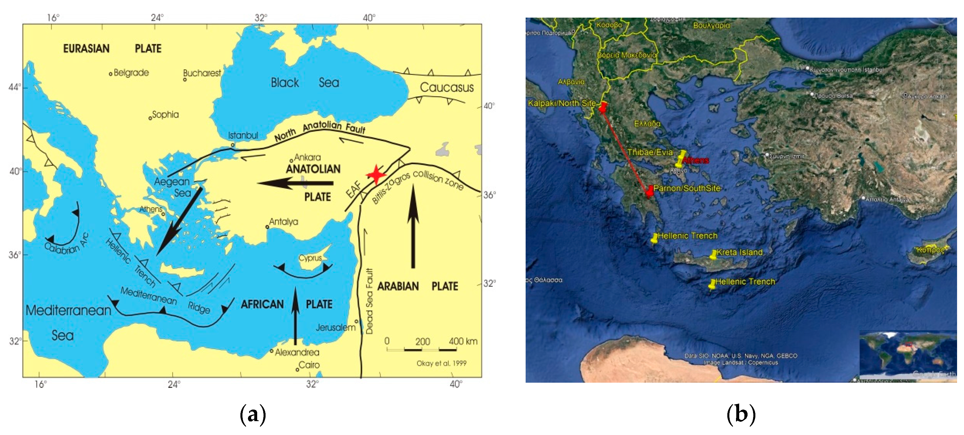
3. Case Study in Greece

Greece, located in the East Mediterranean, experiences a high number of low-to-medium-magnitude earthquakes. This is due to the very active seismic arc known as the Hellenic Trench, located southeast of the island of Crete, where the European and Asiatic tectonic plates collide (Figure 1a,b). Approximately 60% of global seismic activity occurs in this area, with most of it happening in the sea, which protects the wider area from catastrophes. Earthquakes with magnitudes between 3 and 6.5 on the Richter scale, originating from the Hellenic arc or other secondary trenches in the Greek area, occur frequently, making it an important point of research for earthquake prediction.
In our effort to determine whether electro-seismology, particularly ELF waves, can aid in detecting seismic precursors, we proceeded with the installation of two observation sites for ELF recording in the northern and southern regions of mainland Greece. The northern site is situated near the Greek–Albanian border, while the southern site is located close to the top of Mount Parnon, near the town of Sparta. The straight-line distance between the two observation sites is about 340 km, as indicated by the red pins in Figure 1b. Both sites collect ELF data in the frequency range of 2–50 Hz (SR band), with data being collected from 2018 to 2021 at the northern site and from 2020 to the present at the southern site. Extensive descriptions of the systems, technical details, and data recording were presented in previous publications [73,74,75,76].
In this study, we focus on the southern site due to the high number of earthquakes occurring around it, most of which take place in the sea, posing additional difficulties in their estimation. The southern site offers an added advantage over the northern one: a second system of ELF recordings installed by the AGH University of Krakow is hosted there. Each system was designed completely independently by two different research teams, both with extensive experience in ELF measurements. Additionally, both systems were extensively tested by running simultaneous measurements, first in the same location and then in different locations. Simultaneous measurements of the same event taken at the same location with different measurement systems allow us to exclude instrumental effects. Additionally, prior to this study, we tested the response of our systems to various human-made noises to be able to easily recognize them in the recording and not confuse them with pre-seismic signals. Articles [77,78] explain, in detail, the various tests we conducted and the recordings we obtained, which helped us to separate possible precursor signals from anthropogenic noises.
Figure 2 presents recording samples from both systems collecting data at the southern site.
The upper panels in Figure 2 show the recorded signal. The spikes originate from lightning discharges. Their amplitude depends on how powerful the recorded lightning was and how close to the measurement site it occurred. The recorded amplitude and shape of the impulse also depend on the recording system. In particular, the larger the system bandwidth, the larger the recorded amplitude and, therefore, the signal-to-noise ratio. The system bandwidth has to be taken into account when reconstructing the parameters of the source signal. The bottom panels in Figure 2 show the spectra obtained from the recorded signal. We can see that the Schumann resonances at frequencies of about 8, 14, and 21 Hz are clearly visible in the spectra obtained from both systems. Since the bandwidth of the Polish system is larger, in the obtained spectrum, we can also see the higher Schumann resonance modes close to 28, 31, and 39 Hz (bottom panel in Figure 2b).
Figure 3 presents typical examples of possible seismic precursor signals. These signals were detected in most EQ cases from a few days to three weeks before the main shock. The main characteristics of these signals are particular perturbations that appear in the raw data and a significant enhancement of the relevant spectrum around the third Schumann resonance (20–25 Hz).
The raw data, which look very similar to a classical seismogram, led us to suspect that these quasi-seismic signals may have been caused either by ground vibrations due to a forthcoming EQ or by some other anthropogenic effect. To clarify the cause of these signals, we generated various artificial noises, such as knocks, car engines, and gunshots, to check how they would affect the ELF recordings [77,78].
Figure 4 presents the recordings we obtained after vibrating the coils by hand. Figure 3 and Figure 4 demonstrate substantial differences. The upper panels, where the raw data are depicted, demonstrate some similarities, while the lower panels, where the relevant spectra are depicted, appear quite different. In the upper panels of Figure 4, we can see raw data stripes similar to those in Figure 3, but the spectra in the lower panels are quite different. In Figure 4, we can see a very large increase in the spectral power in the lowest part of the spectrum, while in Figure 3, we can see a large spectral power increase in the important range between 20 and 30 Hz. This provides convincing evidence that the pre-seismic-like signals in Figure 3 do not result directly from the ground vibrations.
Further evidence that ground vibrations do not produce seismic-like signals is the duration of the raw data perturbations related to these signals. A typical EQ lasts for about 10 s, which in extreme cases can be extended to 20–30 s. However, in the case of quasi-seismic signals, the raw data perturbations last from 70 to 150 s, which is seven to eight times longer than the duration of a typical EQ.
It would be interesting to answer the question of whether these signals are locally created in the frame of the LAIC idea or an extended phenomenon that could be detected at the same time by remote observation sites.
In the left panel of Figure 5, we present a clear quasi-seismic precursor signal recorded at the site of Parnon by the Polish and the Greek systems simultaneously (middle and lower panels, respectively). At the same time, nothing interesting was recorded far away (~1000 km) at the Polish site of Hylaty (upper panel). The right panel of Figure 5 presents the recordings from the next data file at both sites, Parnon and Hylaty.
Figure 5 presents clear evidence that quasi-pre-seismic signals are local, very short, and independent of sites, time, or general ionospheric disturbances. The signal was clearly recorded in the site of Parnon by both systems, Greek and Polish, but nothing was recorded in the Polish system in Hylaty. Four days after these signals, an EQ of magnitude 5.0 occurred close to the Greek town of Itea, 110 km north of Parnon (case no. 67 in Table 1).
The extended analysis of several EQs that occurred in the Greek area recorded in both sites in the north and south made us formulate the following empirical rules: a seismic precursor, like those shown in Figure 3 and Figure 5, could be seriously considered under the following limitations:
  • An EQ must have a magnitude greater than M4.0;
  • The seismic epicenter must be located within 250–300 km from the observation site;
  • We must perform different studies for EQs that occur on land and at sea.
In Table 1, we show all EQs stronger than M3.3 that occurred during the time span 2020–2022 within a radius of 300 Km around our south observational site of Parnon. Although we set a lower limit of M 4.0, we also included some EQs of lower magnitude because they occurred a few days before or after a stronger EQ or were meta-earthquakes of a main EQ.
Based on the summary of earthquakes and precursor signals presented above, the following results could be established:
  • EQ occurrences further than 250–300 km from the observation site, particularly those that occur in the sea, do not have detectable signals. Cases 10, 23, 33, 37, 42, 47, 51, 55, 57, 68, 73, and 75, as well as EQs with magnitudes less than M4.0, such as cases 7, 18, 25, 43, and 54, belong to this group.
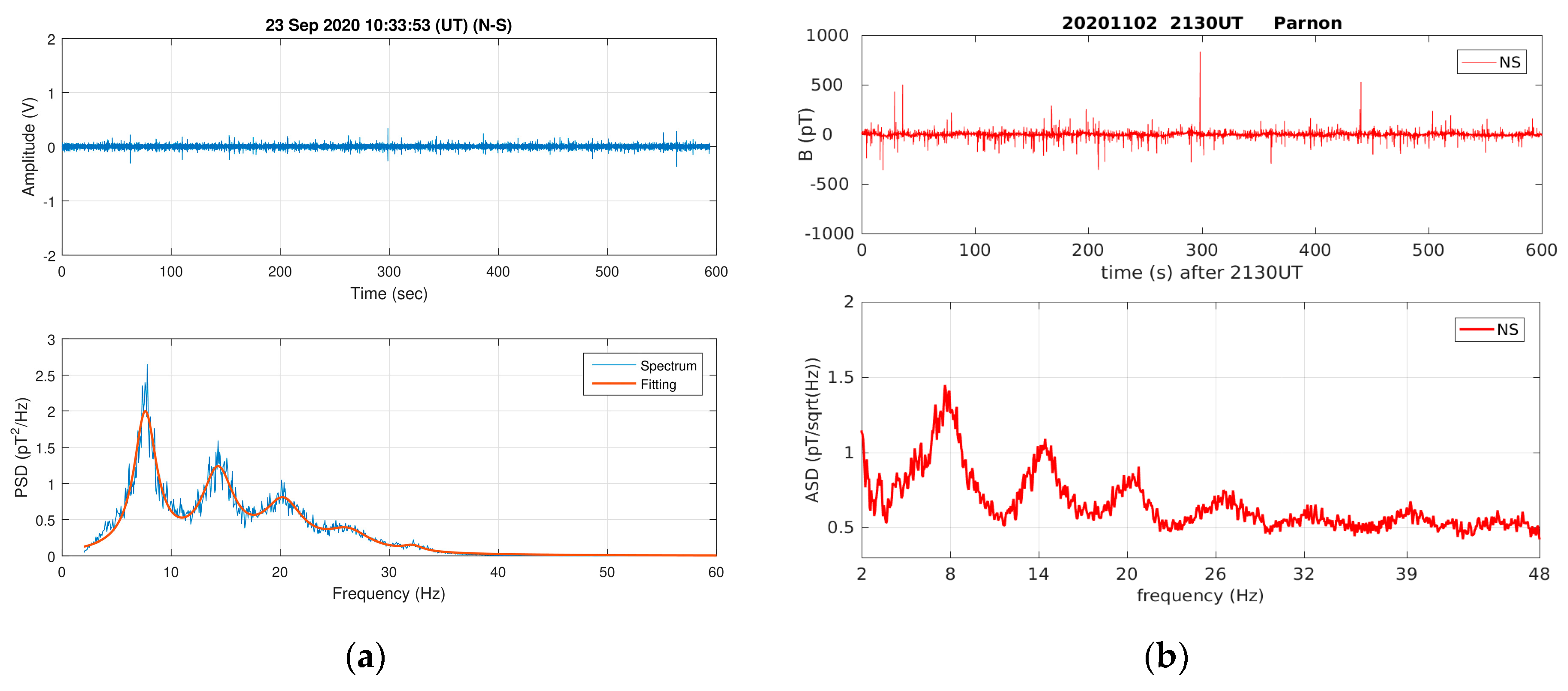
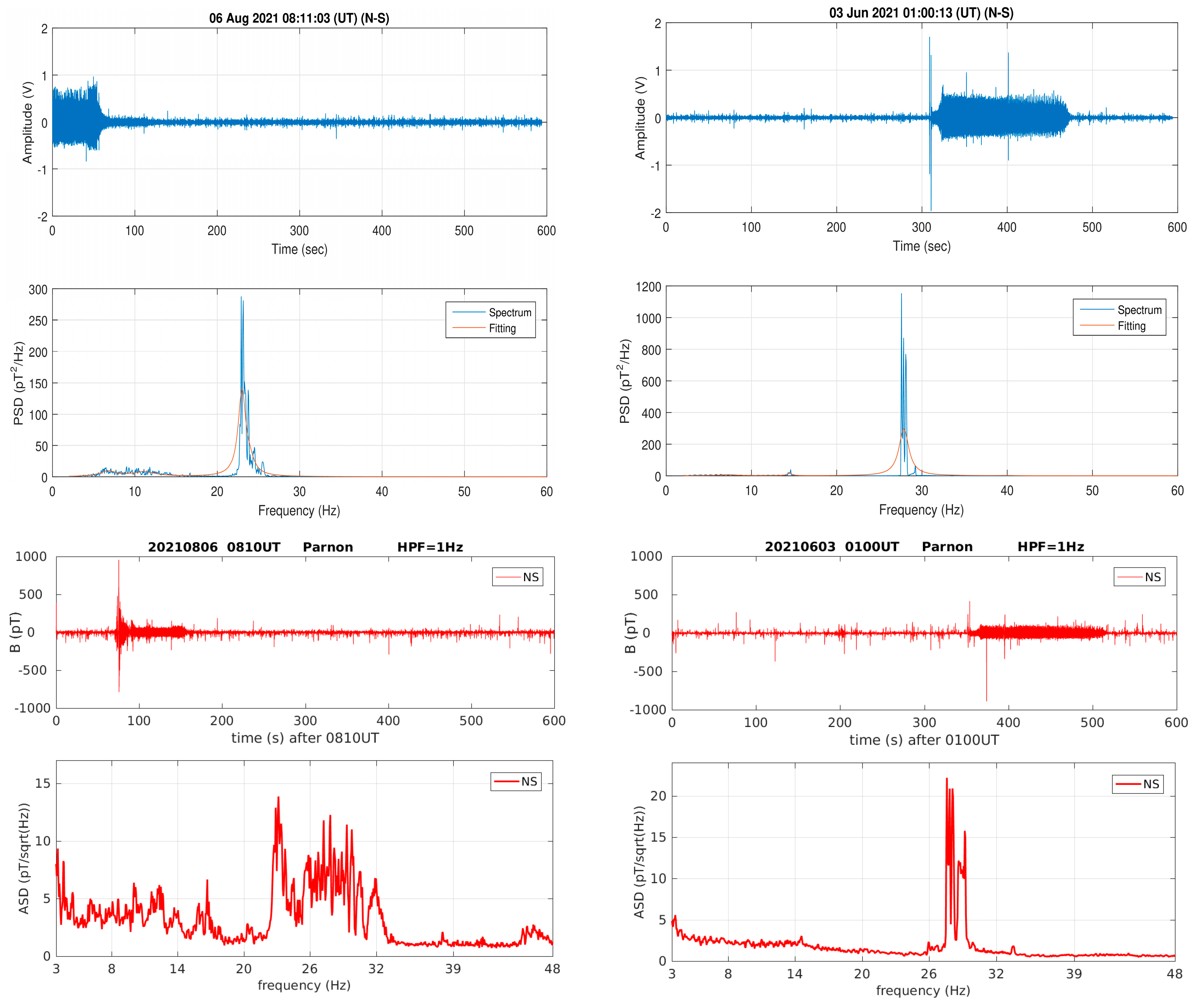
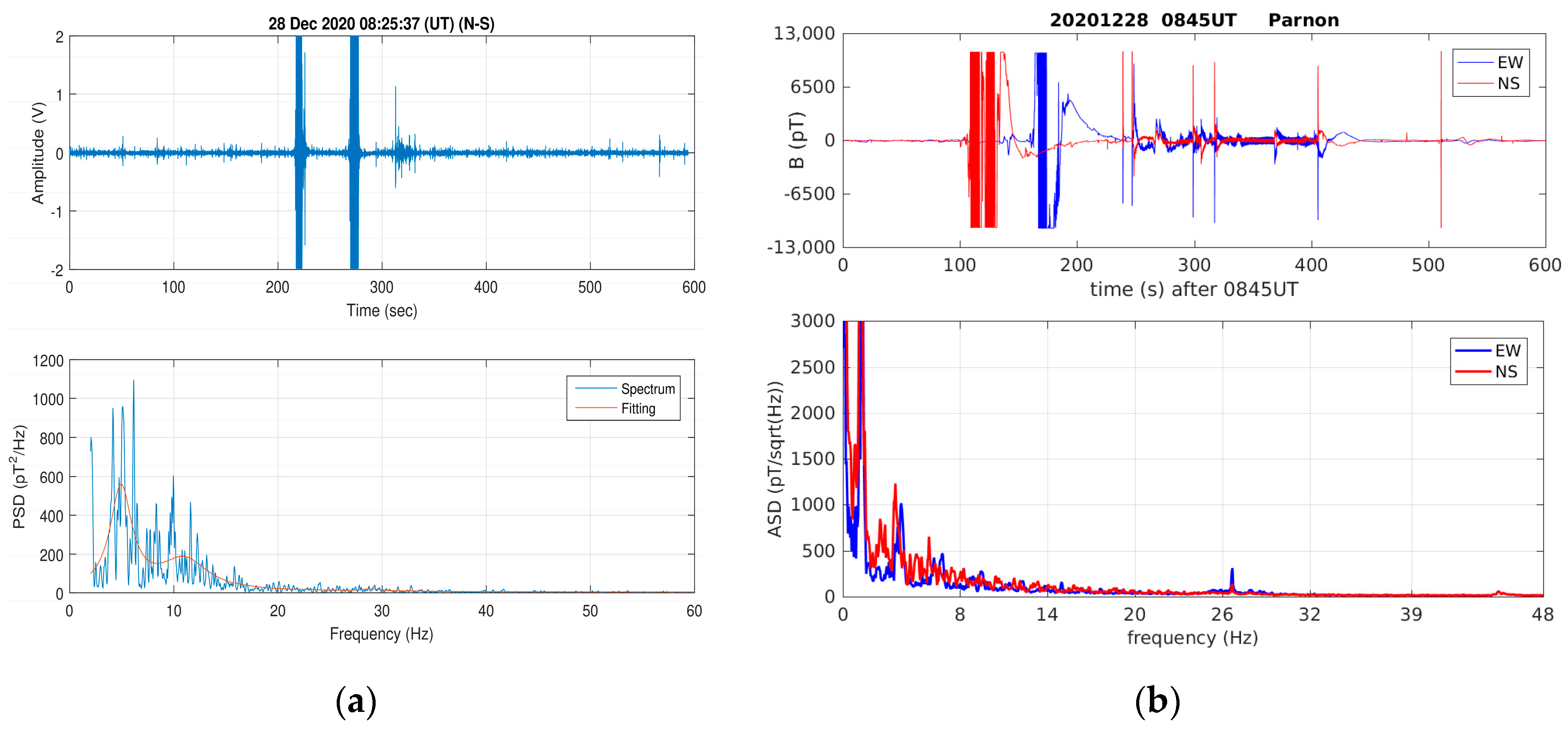
  • Typical quasi-seismic signals appear from a few days to almost three weeks before a main EQ occurrence that has a magnitude higher than M4.0 and a distance shorter than 250–300 km from the observational site.
  • No “orphan” signals were detected without the occurrence of an EQ later. This case is discussed further in the following section.

4. Discussion

Table 1 contains seventy-seven (77) low-to-medium-magnitude EQs, ranging from M3.5 to M6.1, which correspond to 25 EQs per year, or 1 every 2 weeks on average. These EQs occurred in southern Greece during three years of seismic activity (2020–2022). Most of them were concentrated in two main groups: the first group was located on the island of Crete, close to the Hellenic trench, which crosses the area southeast of the island, and the second group north/east of Athens in the line Thibae/Evia (green pins on Figure 6). Both groups are located close to the limits of the red circle (Figure 6), i.e., around 250–300 km from the south observation site.
EQs that fulfill the limitations set in the previous section (magnitude higher than M4.0 and distance shorter than 300 km) demonstrate SR perturbations in the ELF recordings, like those shown in Figure 3, up to twenty days before their occurrence. Conversely, no SR perturbations were observed over time periods longer than 20 days.
At first glance, SR perturbations before an EQ could be considered confident candidates for seismic precursors. However, there are several difficulties in nominating these perturbations as such. The main difficulty is that in Greece, several EQs occur within a few days or even the same day, making it difficult to identify and match a certain SR perturbation to a specific EQ. Additionally, the high frequency of EQ occurrences in the south of Greece does not aid in determining whether a signal is incidental or not. In most cases, an EQ is likely to occur within the next three weeks within the empirical distance of 300 km. From this point of view, the east Mediterranean is a rather complicated place to perform this type of research.
If SR perturbations could be investigated in another country where EQs rarely occur, such as countries located around the Carpathian Mountains or some countries in Central or South America, where strong but not frequent EQs occur, then results could be much more reliable. A possible way to evaluate SR perturbations would be to process them in the context of an integrated group of other promising seismic precursor candidates, such as ionospheric perturbations and TEC. SR perturbations seem to be an interesting aspect of the LAIC mechanism, but they require additional study and certification.
A simple scenario of the LAIC mechanism involves accepting that several days before an EQ occurrence, the “preparation area” around the future EQ epicenter experiences preparatory ground micro-vibrations that create a network of ground micro-cracking. Gases emanate from micro-cracklings and ionize the lower layers of the atmosphere. Radon, which is an ionized gas, remains the main candidate among gases emanating from the ground. It can ionize a large atmospheric area from above the future epicenter to the lower ionosphere. The ionization affects the electric conductivity from the ground to the lower ionosphere, thus affecting the electric charge, which creates ionospheric and TEC perturbations or waves that may be identified as seismic activity precursors. This is a raw but very attractive scenario that remains to be validated.
An effective method of seismic forecasting could arise after the simultaneous processing of all the components involved in the above scenario, such as gas emissions from the ground, atmospheric ionization, electric conductivity, atmospheric electric currents, ionospheric perturbations, TECs, and waves. Continuous and simultaneous observations of all the reported seismic precursor candidates and reprocessing by advanced machine learning software loaded with new current data could possibly lead to confident forecasting results.
In addition, several observational sites should be installed approximately every 300 km, which is the empirical distance within which an earthquake can cause ELF perturbations. The location of these sites should be arranged in a way that would allow triangulation and overlapping so that the epicenter location and possibly the magnitude of a forthcoming earthquake can be estimated. However, several difficulties arise in such a project because of conflicts between various prerequisites. SR observation sites should be located far from inhabited and easily accessible areas, as well as any noisy sources like power lines, high-power radio transmitters, and wind generators. It complicates the coexistence of SR equipment and other observing systems that cannot be battery-powered. Under such circumstances, it is almost impossible to select ideal ‘quiet’ observational places, especially when we need several of them.
Finally, it is evident that the integration and accomplishment of such a proposal exceed the activities of a single research group. The contribution of several research groups from different countries is necessary for the operation of reliable seismic activity forecasting. It is hopeful that several researchers already arrived at the same conclusion [29,47].

5. Conclusions

Schumann resonance perturbations are an interesting component of the current LAIC scenario but not the final solution to the seismic forecasting problem. Several limitations, such as the magnitude of an earthquake being higher than M4.0 and the distance of the epicenter being shorter than 300 km from the recording site, may need to be fulfilled in order for a typical pre-seismic signal to be surveyed. The LAIC scenario is constituted by a chain of events which starts from the ground and extends to the lower ionosphere. The seismic precursor recordings of SR are rings which link parts of the LAIC chain. Finally, it seems that trustworthy seismic forecasting results may only be obtained through an integrated project where all the known quasi-precursors will be included. Observations of ionized gases emanating from the ground during the pre-seismic period, correlated conductivity changes of the atmospheric electricity, ionospheric perturbations of the lower layer conductivity, and variations of the ionospheric height should be included in an integrated project. It is hopeful that such projects have started to be formulated [79,80]. We are convinced that a comprehensive program of systematic observations of all the components involved in the LAIC scenario complemented by machine learning analysis could result in effective EQ forecasting.

Author Contributions

Methodology, V.T. and I.C.; software, G.T. and J.M.; validation, V.T. and I.C.; formal analysis, V.T. and J.M.; investigation, V.T. and J.M.; resources S.K.C., J.K. and C.R.; data curation, J.K. and V.C.; writing—original draft preparation, V.T.; writing—review and editing, V.T., J.M., I.C., V.C., G.T. and S.K.C. All authors have read and agreed to the published version of the manuscript.

Funding

This research received no external funding.

Institutional Review Board Statement

Not applicable.

Informed Consent Statement

Not applicable.

Data Availability Statement

The data presented in this study are available on request from the corresponding author. The data are not publicly available due to confidentiality agreement among research collaborators.

Acknowledgments

We would like to thank the forest service of the Lakonia prefecture in the town of Sparta, especially the director G. Zakkas and the forest personnel, S. Petrakos, K. Samartzis, N. Sourlis, and K. Tsagaroulis, for their valuable contribution in the establishment and servicing of our south observation site near the village of Vamvakou, on Mount Parnon. We would also like to thank the residents and the ecclesiastical committee of the town of Doliana in Northern Greece for offering the necessary accommodation needed for the establishment of our north observation site. Finally, we would like to express a warm thank you to the Mariolopoulos–Kanaginis Foundation for Environmental Sciences for initial financial support, as well as to the Research Committee of the Academy of Athens for supplementary support. We would also like to thank the residents and the ecclesiastical committee of the town of Doliana in Northern Greece, especially the high school’s principal, G. Skordos, for offering the necessary accommodation needed for the establishment of our north observation site.

Conflicts of Interest

The authors declare no conflict of interest.

References

  1. Davis, K.; Baker, D.M. Ionospheric effects observed around the time of the Alaska earthquake of 28 March 1964. J. Geophys. Res. 1965, 70, 2251–2253. [Google Scholar] [CrossRef]
  2. Leonard, R.S.; Barnes, R.A., Jr. Observation of ionospheric disturbances following the Alaska earthquake. JGR Lett. 1965, 70, 1250–1253. [Google Scholar] [CrossRef]
  3. Hayakawa, M.; Fujinawa, Y. (Eds.) Electromagnetic Phenomena Related to Earthquake Prediction; Terra Scientific Publishing Company: Syracuse, NY, USA, 1994. [Google Scholar]
  4. Hayakawa, M.; Molchanov, O. (Eds.) Seismo-Electromagnetics: Lithosphere-Atmosphere-Ionosphere Coupling; Terra Scientific Publiching Company: Tokyo, Japan, 2002. [Google Scholar]
  5. Hayakawa, M.; Molchanov, O.A. Seismo-electromagnetics: As a new field of radiophysics: Electromagnetic phenomena associated with earthquakes. Radio Sci. Bull. 2007, 320, 8–17. [Google Scholar]
  6. Pullinets, A.S. Lithosphere-Atmosphere-Ionosphere Coupling Related to Earthquakes. In Proceedings of the 2nd URSI AT-OASC, Gran Canaria, Spain, 28 May–1 June 2018. [Google Scholar]
  7. Pulinets, S.; Ouzounov, D. Intergeospheres Interaction as a source of earthquake precursor’s generation. In Proceedings of the EMSEV 2018 International Workshop, Potenza, Italy, 17–21 September 2018. [Google Scholar]
  8. Zhao, B.; Qian, C.; Yu, H.; Liu, J.; Maimaitusun, N.; Yu, C.; Zhang, X.; Ma, Y. Preliminary Analysis of Ionospheric Anomalies before Strong Earthquakes in and around Mainland China. Atmosphere 2022, 13, 410. [Google Scholar] [CrossRef]
  9. Hayakawa, M.; Tomakazu, A.; Rozhnoi, A.; Solovieva, M. Very -low -to Low -Frequency Sounding of Ionospheric Perturbations and Possible Association with Earthquakes. In Pre-Earthquake Processes: A Multidisciplinary Approach to Earthquake Prediction Studies; Geophysical Monograph 234; AGU: Washington, DC, USA, 2018; pp. 277–304. [Google Scholar]
  10. Pulinets, S.; Boyarsschuc, X.X. Ionospheric Precursors of Earthquakes; Springer: Berlin/Heidelberg, Germany, 2004; Volume 3, p. 15. [Google Scholar]
  11. Hayakawa, M. Earthquake precursor studies in Japan. In Pre-Earthquake Processes: A Multidisciplinary Approach to Earthquake Prediction Studies; Geophysical Monograph 234; AGU: Washington, DC, USA, 2018; pp. 7–18. [Google Scholar]
  12. Schvets, A.V.; Hayakawa, M.; Meakana, S. Results of sub-ionospheric radio LF monitoring prior to the Tokachi (M = 8, Hokkaido, 25 September 2003) earthquake. Nat. Hazards Earth System Sci. 2004, 4, 647–653. [Google Scholar] [CrossRef]
  13. Namgaladge, A.; Karpov, M.; Knyazeva, M. Seismogenic disturbances of the ionosphere during high geomagnetic activity. Atmosphere 2019, 10, 359. [Google Scholar] [CrossRef]
  14. Schvets, A.V.; Hayakawa, M.; Molchanov, O.A.; Ando, Y. A study of ionospheric response to regional seismic activity by VLF radio sounding. Phys. Chem. Earth 2004, 29, 627–637. [Google Scholar] [CrossRef]
  15. Sorokin, M.V.; Pokhotelov, A.O. Gyrotropic Waves in the mid-latitude ionosphere. J. Atmos. Sol. Terr. Phys. 2005, 67, 921–930. [Google Scholar] [CrossRef]
  16. Hayakawa, M.; Ohta, K.; Sorokin, M.V.; Yaschenko, K.A.; Izutsu, J.; Hobara, Y.; Nickolaenko, P.A. Interpretation in terms of gyrotropic waves of Schumann–resonance-like line emissions observed at Nakatsugawa in possible association with nearby Japanese earthquakes. J. Atmos. Terrestrial Phys. 2010, 72, 1292–1298. [Google Scholar] [CrossRef]
  17. Chakrabarti, S.; Saha, M.; Khan, R.; Mandal, S.; Acharyya, K.; Saha, R. Possible detection of ionospheric disturbances during Sumatra Andaman islands earthquakes in December. Indian J. Radio Space Phys. 2005, 34, 314–317. [Google Scholar]
  18. Sorokin, V.M.; Hayakawa, M. On the generation of narrow-banded ULF/ELF pulsations in the lower ionospheric conducting layer. J. Geophys. Res. 2008, 113, A06306. [Google Scholar] [CrossRef]
  19. Chakrabarti, S.K.; Sasmal, S. Ionospheric anomaly due to seismic activities—Part 2: Evidence from D-layer preparation and disappearance times. Nat. Hazards Earth Syst. Sci. 2010, 10, 1751–1757. [Google Scholar] [CrossRef]
  20. Tao, D.; Wang, G.; Zong, J.; Wen, Y.; Cao, J.; Battiston, R.; Zeren, Z. Are the Significant Ionospheric Anomalies Associated with the 2007 Great Deep –Focus Undersea Jakarta-Java Earthquake? Remote Sens. 2022, 14, 2211. [Google Scholar] [CrossRef]
  21. Harrison, G.R.; Aplin, L.K.; Rycroft, J.M. Atmospheric electricity coupling between earthquake regions and the ionosphere. J. Atmos. Sol. Terr. Phys. 2010, 72, 376–381. [Google Scholar] [CrossRef]
  22. Munawar, S.; Shuanggen, J. Pre-seismic ionospheric anomalies of the 2013 Mw 7.7 Pakistan earthquake from GPS and COSMIC observations. Geod. Geodyn. 2018, 9, 378–387. [Google Scholar]
  23. Nayak, K.; López-Urías, C.; Romero-Andrade, R.; Sharma, G.; Guzmán-Acevedo, G.M.; Trejo-Soto, M.E. Ionospheric Total Electron Content (TEC) Anomalies as Earthquake Precursors: Unveiling the Geophysical Connection Leading to the 2023 Moroccan 6.8 Mw Earthquake. Geosciences 2023, 13, 319. [Google Scholar] [CrossRef]
  24. Liu, J.Y.; Chuo, Y.J.; Shan, S.J.; Tsai, Y.B.; Chen, Y.I.; Pulinets, S.A.; Yu, S.B. Pre-earthquake ionospheric anomalies registered by continuous GPS TEC measurements. Ann. Geophys. 2004, 22, 1585–1593. [Google Scholar] [CrossRef]
  25. Tsugawa, T.; Saito, A.; Otsuka, Y.; Nishioka, M.; Maruyama, T.; Kato, H.; Nagatsuma, T.; Murata, K.T. Ionospheric disturbances detected by GPS total electron content observation after the 2011 off the Pacific coast of Tohoku Earthquake. Earth Planets Space 2011, 63, 875–879. [Google Scholar] [CrossRef]
  26. Dong, L.; Zhang, X.; Du, X. Analysis of Ionospheric precursors possibly related to Yangbi Ms 6.4 and Maduo Ms 7.4 earthquake occurred on 21st May, 2021 in China by GPS TEC and GIM TEC data. Atmosphere 2022, 13, 1725. [Google Scholar] [CrossRef]
  27. Walker, S.N.; Kadirkamanathan, V.; Pokhotelov, O.A. Changes in the ultra-low frequency wave field during the precursor phase to the Sichuan earthquake: DEMETER observations. Ann. Geophys. 2013, 31, 1597–1603. [Google Scholar] [CrossRef]
  28. Parrot, M.; Li, M. Demeter Results Related to Seismic Activity. URSI Radio Sci. Bull. 2017, 88, 18–25. [Google Scholar]
  29. Li, M.; Shen, X.; Yu, C.; Zhang, X. Primary joint statistical seismic influence on ionospheric parameters recorded by the CSES and DEMETER satellites. J. Geophys. Res. Space Phys. 2020, 125, e2020JA028116. [Google Scholar] [CrossRef]
  30. De Santis, A.; Balasis, G.; Pav´on-Carrasco, F.J.; Cianchini, G.; Mandea, M. Potential earthquake precursory pattern from space: The 2015 Nepal event as seen by magnetic Swarm satellites. Adv. Space Res. 2017, 461, 119–126. [Google Scholar] [CrossRef]
  31. Li, M.; Yang, Z.; Song, J.; Zhang, Y.; Jiang, X.; Shen, X. Statistical Seismo-Ionospheric influence with focal Mechanism under consideration. Atmosphere 2023, 14, 455. [Google Scholar] [CrossRef]
  32. Florios, K.; Contopoulos, I.; Christofilakis, V.; Tatsis, G.; Chronopoulos, S.; Repapis, C.; Tritakis, V. Pre-seismic Electromagnetic Perturbations in Two Earthquakes in Northern Greece. Pure App. Geophys. 2020, 177, 787–799. [Google Scholar] [CrossRef]
  33. Florios, K.; Contopoulos, I.; Tatsis, G.; Christofilakis, V.; Chronopoulos, S.; Repapis, C.; Tritakis, V. Possible earthquake forecasting in a narrow space-time-magnitude window. Earth Sci. Inform. 2020, 14, 349–364. [Google Scholar] [CrossRef]
  34. Karamanos, K.; Peratzakis, A.; Kapiris, P.; Nikolopoulos, S.; Kopanas, X.; Eftaxias, K. Extractihg preseismic electromagnetic, signatures in terms of symbolic dynamics. Nonlinear Process. Geophys. 2005, 12, 835–848. [Google Scholar] [CrossRef]
  35. Karamanos, K. Preseismic electromagnetic signals in terms of complexity. Phys. Rev. E 2006, 74, 016104. [Google Scholar] [CrossRef] [PubMed]
  36. Karamanos, K.; Dakopoulos, D.; Aloupis, K.; Peratzakis, A.; Athanasopoulou, S.; Nikolopoulos, S.; Kapiris, P.; Eftaxias, K. Study of pre-seismic Electromagnetic signals in terms of complexity. Phys. Rev. E 2005, 74, 016104/1–21. [Google Scholar] [CrossRef]
  37. Schumann, W.O. On the free oscillations of a conducting sphere which is surrounded by an air layer and an ionosphere shell. Z. Naturforschaftung 1952, 7a, 149–154. (In German) [Google Scholar] [CrossRef]
  38. Balser, M.; Wagner, C. Observations of Earth–Ionosphere Cavity Resonances. Nature 1960, 188, 638–641. [Google Scholar] [CrossRef]
  39. Balser, M.; Wagner, C.A. Diurnal power variations of the Earth-ionosphere cavity modes and their relationship to worldwide thunderstorm activity. JGR 1962, 67, 619–625. [Google Scholar] [CrossRef]
  40. Williams, E.R. The Schumann Resonance: A Global Tropical Thermometer. Science 1992, 256, 1184–1187. [Google Scholar] [CrossRef] [PubMed]
  41. Nickolaenko, P.A.; Hayakawa, M. Schumann Resonance for Tyros; Springer Geophysics: Berlin/Heidelberg, Germany, 2014. [Google Scholar]
  42. Nickolaenko, P.A.; Hayakawa, M. Resonances in the Earth-Ionosphere Cavity; Kluwer Academic Publishers: Amsterdam, The Netherlands, 2002. [Google Scholar]
  43. Galejs, J. Schumann Resonance. Radio Sci. J. Res. NBS/USNC-URSI 1965, 69D, 1043–1055. [Google Scholar] [CrossRef]
  44. Simoes, F.; Pfaff, R.; Berthelier, J.-J.; Klenzing, J. A Review of low Frequency Electromagnetic Wave Phenomena Related to Tropospheric Coupling Mechanisms. Space Sci. Rev. 2012, 168, 551–593. [Google Scholar] [CrossRef]
  45. Price, C.; Melnikov, A. Diurnal, Seasonal and Inter-annual variations in the Schumann resonance parameters. J. Atmos. Sol-Terr. Phys. 2004, 66, 1179–1185. [Google Scholar] [CrossRef]
  46. Nickolaenko, P.A.; Galuk, P.Y.; Hayakawa, M. The effect of a compact ionosphere disturbance over the earthquake: A focus on Schumann resonance. Int. J. Electron. Appl. Res. 2018, 5, 181444053. [Google Scholar] [CrossRef]
  47. Schekotov, A.; Chebrov, D.; Hayakawa, M.; Belyaev, G.; Berseneva, N. Short-term earthquake prediction in Kamchatka using low-frequency magnetic fields. Nat. Hazards 2020, 100, 735–755. [Google Scholar] [CrossRef]
  48. Sekiguchi, M.; Hobara, Y.; Hayakawa, M. Diurnal and seasonal variations in the Schumann resonance parameters at Moshiri, Japan. J. Atmos. Electr. 2008, 28, 1–10. [Google Scholar] [CrossRef]
  49. Sentman, D.D. Magnetic elliptical polarization of Schumann resonances. Radio Sci. 1987, 22, 595–606. [Google Scholar] [CrossRef]
  50. Roldugin, V.C.; Maltsev, Y.P.; Petrova, G.A.; Vasiljev, A.N. Decrease of the first Schumann resonance frequency during solar proton events. J. Geophys. Res. 2001, 106, 18555–18562. [Google Scholar] [CrossRef]
  51. Shvets, A.V.; Nickolaenko, A.P.; Belyaev, G.G.; Schekotov, A.Y. Analysis Schumann Resonance Parameter Variations Associated with Solar Proton Events. Telecommun. Radio Eng. 2005, 64, 771–791. [Google Scholar] [CrossRef]
  52. Huang, E.; Williams, E.; Boldi, R.; Heckman, S.; Lyons, W.; Taylor, M.; Nelson, T.; Wong, C. Criteria for sprites and elves based on Schumann resonance observations. J. Geophys. Res. Atmos. 1999, 104, 16943–16964. [Google Scholar] [CrossRef]
  53. Yang, H.; Pasko, V.P. Power “variations of Schumann resonances related to El Nino and La Nina phenomena”. Geophys. Res. Lett 2007, 34, 1102. [Google Scholar] [CrossRef]
  54. Wever, R.A. The Circadian System of Man. Results of Experiments under Temporal Isolation; Springer: Berlin/Heidelberg, Germany, 1979; pp. 17–24. [Google Scholar]
  55. Wever, R. The effects of electric fields on circadian rhythmicity in men. Life Sci Space Res. 1970, 8, 177–187. [Google Scholar] [PubMed]
  56. Panagopoulos, D.J.; Balmori, A. On the biophysical mechanism of sensing atmospheric discharges by living organisms. Sci. Total. Environ. 2017, 599-600, 2026–2034. [Google Scholar] [CrossRef] [PubMed]
  57. Panagopoulos, D.J.; Chrousos, G.P. Shielding methods and products against man-made Electromagnetic Fields: Protection versus risk. Sci. Total. Environ. 2019, 667, 255–262. [Google Scholar] [CrossRef] [PubMed]
  58. Fdez-Arroyabe, P.; Fornieles-Callejón, J.; Santurtún, A.; Szangolies, L.; Donner, R.V. Schumann Resonance and cardiovascular hospital admission in the area of Granada, Spain: An event coincidence analysis approach. Sci. Total Environ. 2020, 705, 135813. [Google Scholar] [CrossRef] [PubMed]
  59. Elhalel, G.; Price, C.; Fixler, D.; Shainberg, A. Cardioprotection from stress conditions by weak magnetic fields in the Schumann Resonance band. Sci. Rep. 2019, 9, 1645. [Google Scholar] [CrossRef] [PubMed]
  60. Nieckarz, Z.; Kułak, A.; Zięba, S.; Michalec, A. Day-to-Day Variation of the Angular Distribution of Lightning Activity Calculated from ELF Magnetic Measurements. Coupling of thunderstorms and lightning discharges to near-earth space. In Proceedings of the Workshop, Corte, France, 23–27 June 2008; pp. 28–33. [Google Scholar]
  61. Mlynarczyk, J.; Kulak, A.; Salvador, J. The Accuracy of Radio Direction Finding in the Extremely Low Frequency Range. Radio Sci. 2017, 52, 1245–1252. [Google Scholar] [CrossRef]
  62. Yagova, N.V.; Sinha, A.K.; Pilipenko, V.A.; Fedorov, E.N.; Holzworth, R.; Vichare, G. ULF electromagnetic noise from regional lightning activity: Model and observations. J. Atmos. Sol. Terr. Phys. 2018, 182, 223–228. [Google Scholar] [CrossRef]
  63. Schekotov, A.; Pilipenko, V.; Shiokawa, K.; Fedorov, E. ULF impulsive magnetic response at mid-latitudes to lightning activity. Earth Planets Space 2011, 63, 119–128. [Google Scholar] [CrossRef]
  64. Fraser-Smith, A.C. ULF magnetic fields generated by electrical storms and their significance to geomagnetic pulsation generation. Geophys. Res. Lett. 1993, 20, 467–470. [Google Scholar] [CrossRef]
  65. Koloskov, A.V.; Budanov, O.V.; Yampolski, Y.M. Long-term monitoring of the Schumann resonance signals from Antarctica. In Proceedings of the 2014 XXXIth URSI General Assembly and Scientific Symposium (URSI GASS), Beijing, China, 6–23 August 2014; pp. 1–4. [Google Scholar]
  66. Tatsis, G.; Votis, C.; Christofilakis, V.; Kostarakis, P.; Tritakis, V.; Repapis, C. A prototype data acquisition and processing system for Schumann resonance measurements. J. Atmos. Sol. Terr. Phys. 2015, 135, 152–160. [Google Scholar] [CrossRef]
  67. Hobara, Y.; Parrot, M. Ionospheric perturbations linked to a very powerful seismic event. J. Atmos. Sol.-Terr. Phys. 2005, 67, 677–685. [Google Scholar] [CrossRef]
  68. Sinitsind, V.; Gordeev, E.; Hayakawa, M. Seismoionospheric depression of the ULF geomagnetic fluctuations at Kamchatka and Japan. Phys Chem Earth 2006, 31, 313–318. [Google Scholar]
  69. Fidani, C.; Battiston, R. Analysis of NOAA particle data and correlations to seismic activity. Nat. Hazards Earth Syst. Sci. 2008, 8, 1277–1291. [Google Scholar] [CrossRef]
  70. Chowdhury, S.; Kundu, S.; Ghosh, S.; Hayakawa, M.; Schekotov, A.; Potirakis, S.M.; Chakrabarti, S.K.; Sasmal, S. Direct and indirect evidence of pre-seismic electromagnetic emissions associated with two large earthquakes in Japan. Nat. Hazards 2022, 112, 2403–2432. [Google Scholar] [CrossRef]
  71. Christofilakis, V.; Tatsis, G.; Votis, G.; Contopoulos, I.; Repapis, C.; Tritakis, V. Significant ELF perturbations in the Schumann Resonance band before and during a shallow mid-magnitude seismic activity in the Greek area (Kalpaki). J. Atmos. Sol. Terr. Phys. 2019, 182, 138–146. [Google Scholar] [CrossRef]
  72. Tritakis, V.; Contopoulos, I.; Mlynarczyk, J.; Christofilakis, V.; Tatsis, G.; Repapis, C. How Effective and Prerequisite Are Electromagnetic Extremely Low Frequency (ELF) Recordings in the Schumann Resonances Band to Function as Seismic Activity Precursors. Atmosphere 2022, 13, 185. [Google Scholar] [CrossRef]
  73. Tatsis, G.; Christofilakis, V.; Chronopoulos, S.K.; Kostarakis, P.; Nistazakis, H.E.; Repapis, C.; Tritakis, V. Design and Implementation of a Test Fixture for ELF Schumann Resonance Magnetic Antenna Receiver and Magnetic Permeability Measurements. Electronics 2020, 9, 171. [Google Scholar] [CrossRef]
  74. Tatsis, G.; Christofilakis, V.; Chronopoulos, S.K.; Baldoumas, G.; Sakkas, A.; Paschalidou, A.K.; Kassomenos, P.; Petrou, I.; Kostarakis, P.; Repapis, C.; et al. Study of the variations in THE Schumann resonances parameters measured in a Southern Mediterranean environment. Sci. Total Environ. 2020, 715, 136926. [Google Scholar] [CrossRef] [PubMed]
  75. Votis, C.I.; Tatsis, G.; Christofilakis, V.; Chronopoulos, S.K.; Kostarakis, P.; Tritakis, V.; Repapis, C. A new portable ELF Schumann resonance receiver: Design and detailed analysis of the antenna and the analog front-end. J. Wirel. Com Netw. 2018, 2018, 155. [Google Scholar] [CrossRef]
  76. Mlynarczyk, J.; Popek, M.; Kulak, A.; Klucjasz, S.; Martynski, K.; Kubisz, J. New Broadband ELF Receiver for Studying Atmospheric Discharges in Central Europe. In Proceedings of the Baltic URSI Symposium, Poznan, Poland, 14–17 May 2018. [Google Scholar]
  77. Wouters, B.; Gardner, A.S.; Moholdt, G. Global Glacier Mass Loss during the GRACE satellite Mission (2002–2016). Front. Earth Sci. 2019, 7, 96. [Google Scholar] [CrossRef]
  78. Mlynarczyk, J.; Tritakis, V.; Contopoulos, I.; Nieckarz, Z.; Christofilakis, V.; Tatsis, G.; Repapis, C. Anthropogenic Sources of Electromagnetic Interference in the Lowest ELF Band Recordings (Schumann Resonances). Magnetism 2022, 2, 152–167. [Google Scholar] [CrossRef]
  79. Sasmal, S.; Chowdhury, S.; Kundu, S.; Politis, D.Z.; Potirakis, S.M.; Balasis, G.; Hayakawa, M.; Chakrabarti, S.K. Pre-Seismic Irregularities during the 2020 Samos (Greece) Earthquake (M = 6.9) as Investigated from Multi-Parameter Approach by Ground and Space-Based Techniques. Atmosphere 2021, 12, 1059. [Google Scholar] [CrossRef]
  80. Uyanık, H.; Şentürk, E.; Akpınar, M.H.; Ozcelik, S.T.A.; Kokum, M.; Freeshah, M.; Sengur, A. A Multi-Input Convolutional Neural Networks Model for Earthquake Precursor Detection Based on Ionospheric Total Electron Content. Remote. Sens. 2023, 15, 5690. [Google Scholar] [CrossRef]
Figure 1. Maps of the East Mediterranean: (a) the movements of the tectonic plates, the Hellenic trench to the left, and the Anatolian faults to the right are depicted; the red cross indicates the place where the Arabian plate and the Anatolian plate collide and earthquakes often occur. (b) A relief map showing a general view of the most seismic area of the world. Red pins mark our SR observation sites, while yellow pins mark important places. The very active Hellenic trench southeast of the island of Crete is also marked.
Atmosphere 15 00457 g001
Figure 2. Typical ELF recordings obtained from (a) the Greek system and (b) the Polish system. The raw data are shown in the upper panels and the calculated spectra in the frequency range of 2–48 Hz in the lower panels. The Schumann resonances of about 8, 14, 20, 28 Hz are evident in both spectra.
Atmosphere 15 00457 g002
Figure 3. Perturbations in the raw data and spectra, considered quasi-pre-seismic signals. Simultaneous measurements were received by the Greek system (upper panels) and the Polish (lower panels).
Atmosphere 15 00457 g003
Figure 4. Perturbations in raw data (upper panels) and relevant spectra (lower panels) made artificially simulating the ground vibrations by moving the coils by hand. Recordings from (a) the Greek and (b) the Polish system.
Atmosphere 15 00457 g004
Figure 5. Simultaneous recordings in the observation sites of Hylaty (Poland) and Parnon (Greece). Upper panels show the signals recorded by the Polish systems at Hylaty. Middle and lower panels show the signals recorded in Parnon by the Polish and the Greek system, respectively. (a) Quasi-pre-seismic signals observed in Parnon; (b) typical recordings.
Atmosphere 15 00457 g005
Figure 6. Map of southern Greece and the broader area of Eastern Mediterranean. Lower red pin indicates the location of the south observation site on Mount Parnon. The red circle borders an area of 250 km around Parnon, which encircles EQs that occurred within the empirically determined distance of best recording. The two green pins show the locations where successive EQs occurred for several months.
Atmosphere 15 00457 g006
Table 1. Earthquakes of magnitudes M3.3 to M6.1 that occurred during the years 2020–2022 around the south observational site in Greece (Parnon).
NoYear/Month/DayPlace of OccurrenceMagnitude (Richters)Land/Sea/IslandCoordinates
YEAR 2020
0120/02/15Nafpaktos4.5S38.42 N/21.98 E
0220/03/20Parga4.3S39.17 N/20.24 E
0320/03/21Parga5.6S39.16 N/20.23 E
0420/08/09Kyllini4.2S37.85 N/21.11 E
0520/08/17Hydra4.6S37.15 N/23.28 E
0620/09/11Alkyonides4.2S38.65 N/23.34 E
0720/09/11Nafpaktos3.2S38.21 N/21.52 E
0820/09/18Kreta4.1L35.14 N/24.48 E
0920/09/18Kythira5.3S35.54 N/22.49 E
1020/10/12Siteia5.2S35.80 N/26.90 E
1120/12/09Euboia3.9L38.90 N/24.10 E
1220/12/02Thibae4.4L38.19 N/23.25 E
YEAR 2021
1321/01/13Nafpaktos/Aigion4.2S38.19 N/22.04 E
1421/02/17Nafpaktos4.9S38.25 N/22.17 E
1521/03/04Helassona6.1L39.51 N/22.85 E
1621/06/01Helassona4.6L39.83 N/22.07 E
1721/06/03Kalavrita4.8L38.13 N/22.02 E
1821/07/05Herakleio4.2L35.15 N/28.25 E
1921/07/10Thevae3.3L38.32 N/23.33 E
2021/07/11Thibae4.2L38.28 N/22.92 E
2121/07/20Thibae4.5L38.26 N/22.89 E
2221/07/21Herakleio4.8L35.18 N/25.83 E
2321/07/30Thibae4.1L38.35 N/23.36 E
2421/08/01Nisyros5.3S36.40 N/27.06 E
2521/08/11Thibae4.3L38.29 N/20.45 E
2621/08/11Arvi/Kreta3.4L34.98 N/25.26 E
2721/09/02Thibae4.0L35.13 Ν/25.26 Ε
2821/09/12Thibae4.0/3/5L35.18 Ν/25.23 Ε
2921/09/14Zakynthos4.5S37.73 Ν/20.28 Ε
3021/09/27Kreta5.8L35.12 Ν/25.26 Ε
3121/09/27Kreta/Arkalochori5.8L35.85 N/25.15 E
3221/09/28Herakleion5.3S35.15 Ν/25.22 Ε
3321/10/12Kreta6.3S
3421/10/19Karpathos6.1L28.38 Ν/38.84 Ε
3521/12/15Aigio4.2L38.15 N/22.33 E
3621/12/29kreta5.7S35.83 Ν/25.21 Ε
3722/01/02Zakynthos4.1S37.76 N/19.97 E
3822/03/29Amfilochia3.9L38.83 N/21.23 E
3922/04/07Thibae3.9/3.6L38.29 N/23.43 E
4022/04/08Myrtoo4.5S36.57 N/23.38 E
4122/04/08Zakynthos4.0/3.8S37.31 N/20.56 E
4222/04/10Thibae4.3L38.31 N/23.37 E
4322/04/19Santorini3.7S36.48 N/25.44 E
4422/04/27Kalamata3.5S36.69 N/23.09 E
4522/04/27Kythira5.2S35.48 N/22.51 E
4622/05/04Chania/Kreta3.9L35.53 N/23.58 E
4722/05/08Kreta/Arkaloxori4.4L35.15 N/25.31 E
4822/05/22Amfilochia4.3L38.72 N/21.26 E
4922/05/26Gerolimenas4.2S36.36 N/22.20 E
5022/06/04Kreta/Arkalochori3.9L35.13 N/25.30 E
5122/07/17Herakleio3.6L35.16 N/28.26 E
5222/07/13Arkalochori4.1L35.18 N/25.31 E
5322/07/29Marathia4.3S38.41 N/21.99 E
5422/08/12Arkalochori3.5L35.19 N/25.33 E
5522/08/16Kyllini3.6L37.69 N/21.71 E
5622/08/16Preveza4.0L39.20 N/20.60 E
5722/08/30Leykada4.3S38.33 N/20.32 E
5822/08/31Samos4.7/5.7S37.45 N/26.51 E
5922/09/03Thibae3.9L38.33 N/23.37 E
6022/09/03Kreta/Zakros5.2S34.87 N/20.44 E
6122/09/07Monemvasia3.6L36.24 N/22.57 E
6222/09/08Zakynthos5.4S37.87 N/19.93 E
6322/09/24Leykada4.1S38.29 N/20.30 E
6422/09/15Kreta/South3.7S34.36 N/25.33 E
6522/09/19Kreta/Siteia4.2S35.81 N/26.92 E
6622/09/29kreta4.5L35.21 N/2536 E
6722/10/02Kreta/Lasithi5.0S35.79 N/26.88 E
6822/10/08Itea5.0S38.31 N/22.52 E
6922/11/20Kasos5.5Isl.35.72 N/26.54 E
7022/11/29Euboia4.7L38.25 N/24.26 E
7122/12/14Euboia4.3L38.23 N/24.24 E
7222/12/28Euboia/Psachna4.9L38.56 N/23.69 E
7322/12/14Euboia4.3L38.23 N/24.24 E
YEAR 2023
7423/01/04Euboia4.2L38.73 N/23.68 E
7523/01/07Lesbos4.9Isl.39.01 N/26.14 E
7623/01/22Kamena Vourla4.1L35.48 N/22.45 E
7723/01/25Rhodes5.9S36.23 N/28.14 E
Disclaimer/Publisher’s Note: The statements, opinions and data contained in all publications are solely those of the individual author(s) and contributor(s) and not of MDPI and/or the editor(s). MDPI and/or the editor(s) disclaim responsibility for any injury to people or property resulting from any ideas, methods, instructions or products referred to in the content.

