Review

Climatology of the Nonmigrating Tides Based on Long-Term SABER/TIMED Measurements and Their Impact on the Longitudinal Structures Observed in the Ionosphere

National Institute of Geophysics, Geodesy and Geography, Bulgarian Academy of Sciences, Acad. G. Bonchev Str., bl. 3, 1113 Sofia, Bulgaria
*
Author to whom correspondence should be addressed.
Atmosphere 2024, 15(4), 478; https://doi.org/10.3390/atmos15040478
Submission received: 26 February 2024 / Revised: 28 March 2024 / Accepted: 10 April 2024 / Published: 12 April 2024

Abstract

:
This paper presents climatological features of the longitudinal structures WN4, WN3, and WN2 and their drivers observed in the lower thermospheric temperatures and in the ionospheric TEC. For this purpose, two long-term data sets are utilized: the satellite SABER/TIMED temperature measurements, and the global TEC maps generated with the NASA JPL for the interval of 2002–2022. As the main drivers of the longitudinal structures are mainly nonmigrating tides, this study first investigates the climatology of those nonmigrating tides, which are the main contributors of the considered longitudinal structures; these are nonmigrating diurnal DE3, DE2, and DW2, and semidiurnal SW4 and SE2 tides. The climatology of WN4, WN3, and WN2 structures in the lower thermosphere reveals that WN4 is the strongest one with a magnitude of ~20 K observed at 10° S in August, followed by WN2 with ~13.9 K at 10° S in February, and the weakest is WN3 with ~12.4 K observed over the equator in July. In the ionosphere, WN3 is the strongest structure with a magnitude of 5.9 TECU located at −30° modip latitude in October, followed by WN2 with 5.4 TECU at 30 modip in March, and the last is WN4 with 3.7 TECU at −30 modip in August. Both the climatology of the WSA and the features of its drivers are investigated as well.

1. Introduction

Atmospheric tides in the mesosphere and lower thermosphere (MLT), where they attain large amplitudes, play an important role in the general circulation of the atmosphere. The tidal components, which follow the apparent westward propagation of the Sun relative to the Earth’s surface, are called migrating tides, and are a function of local time (LT) alone [1]. They are predominantly forced by solar radiation absorption in the tropospheric water vapor and stratospheric ozone. All non-Sun-synchronous tidal components are called nonmigrating tides [2], or these are all tides propagating eastward, zonally symmetric ones, and those propagating westward but with a different phase speed from that of the apparent motion of the Sun. Nonmigrating tides are thought to have two major sources: nonlinear wave-wave interaction processes in the stratosphere-mesosphere region [3,4,5,6], and the release of latent heat by deep convective clouds in the tropical troposphere [7,8,9,10,11,12]. Deep convection largely depends on land–sea distribution and sea-surface temperatures; hence, such a source of nonmigrating tides leads to their dependence on universal time (UT) and longitude.
The presence of nonmigrating tides in the surface pressure observations was reported first by Chapman and Lindzen, 1970 [1], and further developed by Kato, 1989 [2]. Their detection in the upper levels of the atmosphere, however, was possible only after the advent of global satellite measurements at altitudes where the tidal signal is significantly large in comparison with other variations. It is also important to note that satellite observations allow us to separate the nonmigrating from migrating tides and to study their global structures and temporal variability [5,6,13,14,15,16,17,18,19,20,21]. Based on the above-mentioned studies, it appears that the nonmigrating tides are quite large, and often exceed the corresponding migrating tides in the lower thermosphere [6,16,22,23,24,25]. They lead to longitudinal variations in the local time structures of neutral winds and temperatures in the MLT region [26].
Among the most frequently used space-based instruments for investigating atmospheric tides in the MLT region during the last decade has been the SABER instrument onboard the TIMED satellite, which provides continuous temperature profiles from the lower stratosphere to the lower thermosphere (20–110 km) at middle and low latitudes (±50°). Owing to the orbit design of the satellite, the SABER data of the 60 days resolution has been usually utilized for clarifying the global structures and climatological features of the temperature migrating and nonmigrating tides in the middle atmosphere [20,22,23,27,28,29]. Recently Li et al., 2015 [30], proposed a new approach for extracting the tidal characteristics with 1 day resolution, and particularly investigated the diurnal eastward-propagating tide with zonal wave number 3 (noted as DE3). The authors found that the DE3 components, based on 11 years of observations (2002–2012), are similar to those of previous works [16,27]. Furthermore, Li et al., 2015 [30], reported that the DE3 component is slightly stronger during the eastward wind QBO phase than the westward phase, a result obtained before by Pancheva et al., 2010 and 2014 [27,31]. The same method for extracting the tidal characteristics with 1-day time resolution was applied by Li et al., 2017 [32], to study the semidiurnal eastward propagating tide with zonal wavenumber 2 (marked as SE2) tide; again, it was found that the climatology is analogous of the previous result presented by Pancheva et al., 2010 [27], and Pancheva and Mukhtarov, 2011 [21]. Very recently, Li et al., 2023 [33], reported the climatology and QBO influence on the nonmigrating DE3 tide in the zonal wind extracted with 1-day resolution from the TIDI instrument onboard the TIMED satellite. Through comparative analysis, the authors obtained the result that the long-term variations in DE3 in temperature and zonal wind are consistent with each other; this indicates that the long-term dominant dynamic processes of DE3 in the temperature and zonal wind components are similar.
The advent of new satellite missions over the past decade resulted in more deeply understanding the coupling between the terrestrial atmosphere and ionosphere-thermosphere (IT) system. The conventional sources of ionospheric structure and variability are related to changes in solar radiative output and geomagnetic activity, together with the subsequent response of the IT system and interaction between the components. The high sensitivity of the ionosphere to the external solar forcing causes its rapid and significant variability on time scales ranging from minutes to a solar cycle. To understand and forecast such large ionospheric variability is one of the main tasks of space weather research due to the increasing importance of satellite-based communications and positioning, as well as because of the potential to affect the reliable performance of some technological systems operating in space and on the Earth. A variety of new evidence obtained recently demonstrated unambiguously that a substantial amount of the IT variability also owes to waves forced in the lower parts of the atmosphere [34,35,36,37]. The latter contradicts to previous textbook knowledge that the IT system variability can be driven only by solar and geomagnetic activity. The primary mechanism through which energy and momentum are transferred from the lower atmosphere is through the propagation and dissipation of atmospheric waves, including electrodynamic coupling through dynamo processes. Therefore, attention is now being directed not only to forcing from above, but also towards the impact of the processes from below to the IT system.
The solar thermal tides usually dominate the large-scale atmospheric fields in the lower thermosphere. However, due to increasing eddy and molecular dissipation, this is a region where the atmospheric tides propagating from below usually dampen. By depositing their net momentum and energy into the mean flow, the mean circulation can be modified. By mixing the atmospheric species there or in nonlinear interactions with other waves, the tides can affect the wind fields, the density of different neutral species, or the energy budget. The tides penetrating into the ionospheric E region can affect the overlying ionosphere F-region by the “E-region wind dynamo”. In this way, the neutral dynamics converts the lower thermosphere into the strongest driver from below of the ionosphere F-region. The “E-region wind dynamo”, by sequence of processes described in detail in [23,38,39], produce the equatorial ionization anomaly (EIA) near ±15–20° dip latitude. Additionally, the atmospheric tides can also propagate directly up to thermospheric heights [40,41]. Therefore, either through complex coupling mechanisms or through direct propagation, the MLT tides can affect the whole ionosphere-thermosphere system. As mentioned above, the nonmigrating tides give rise to longitudinal structures in local time in both the MLT region and the ionosphere. Therefore, the role of the nonmigrating tides as a possible link between the troposphere and ionosphere has attracted many scientists recently.
Over the last decade, new observational evidence demonstrated the terrestrial weather impacts on the ionosphere. Such evidence is the longitudinal WN3 or WN4 structures, which are suggested to be caused by different atmospheric nonmigrating tides and zonally planetary waves. Sagawa et al., 2005 [34], observed four enhanced longitudinal regions of the nighttime airglow intensity in the EIA, and pointed out that this plasma density WN4 structure is most probably forced by the nonmigrating tides from below, which modulate the E-region dynamo electric field. Later Immel et al., 2006 [35] and England et al., 2006 [42], specified that the diurnal eastward-propagating zonal wave number 3 (DE3) tide is responsible for the generation of the ionospheric WN4 structure. We note that, at a fixed local time, the DE3 wave is seen as four maxima on longitude in all tidal fields. The WN4 structure has also been observed in E × B plasma drift [36,37,43,44] and in the equatorial electrojet (EEJ) [45,46]. The satellite observations of different ionospheric and thermospheric parameters, such as Total Electron Content (TEC), the electron temperature, F-region zonal neutral wind and neutral mass density, and the ionospheric F2 layer height (hmF2), have also shown WN4 longitudinal structures [26,47,48,49,50,51,52,53,54,55,56].
The above-mentioned observational evidence illustrating the MLT wave impacts on the ionosphere demonstrated only the ionospheric response without the attendant forcing event from below. Pancheva and Mukhtarov, 2010 [26], presented, for the first time, the global structure and seasonal variability of the ionospheric response to the forced-from=below nonmigrating tides DE3 and DE2 (diurnal tide eastward propagating with zonal wavenumber 2), which generate WN4 and WN3 both in the MLT temperature field and in the ionospheric hmF2. Later, by using the FORMOSAT-3/COSMIC (F3/C) electron density profiles and the SABER temperatures, Mukhtarov and Pancheva, 2011 [56], utilized them to define the latitude and altitude structures of the ionospheric DE3 and DE2 tidal response to the DE3 and DE2 temperature tides coming from below. An interesting result is the observed two altitude regions of enhanced electron density response: an upper level response maximizing near 400–450 km, and a bottom level one below 250–300 km. Both regions revealed different phase structures, indicating that the upper level response is mainly due to the DE3/DE2-modulated vertical plasma drift, while the bottom level one is complex and caused by more than one mechanism.
The next step in studying the ionospheric response to the tidal forcing from below was done by a detailed comparison between the simulated and observed global electron density response to different atmospheric tides forced from below. Such a comparison, reported by Pancheva et al., 2012 [57], was presented for the first time. For this purpose, the authors used the SABER temperature tidal forcing and the F3/C electron density response for the period of time October 2007 to March 2009, as well as the Earth’s whole atmospheric model from the troposphere to the ionosphere, called GAIA [58,59,60], for the simulation of the electron density tidal responses. In general, the GAIA model reproduced the F3/C DE3/DE2 responses quite well, particularly the DE3 response. Regarding the altitude structure of the DE3/DE2 response, the simulations indicated that, while the upper level DE3/DE2 response is apparently shaped mainly by the “fountain effect”, the reason(s) for the lower level is not very clear. It could be a possible direct tidal effect in the considered altitude, mainly due to the vertical wind DE3 tide, or a possible coupling between tides and the ionosphere via changes in neutral density, and particularly a modification of [O] and mass mixing ration of [O] (measured in kg/kg).
All of the above-mentioned studies indicated that the WN4 longitudinal structure is a prominent feature of the low-latitude ionosphere-thermosphere system, and in general it can be reproduced by the models [61,62,63]. However, when a given ionospheric longitudinal structure is investigated only at fixed local times (LT), it cannot be directly related to a certain tidal component. For example, if we consider only diurnal and semidiurnal tides, the WN4 structure can be forced by DE3, DW5, SW6, SE2, and SPW4 (according to the standard nomenclature S corresponds to semidiurnal tide, while W/E to westward/eastward propagation; SPW means the stationary planetary wave), and the WN3 structure by DW4, DE2, SW5, SE1, and SPW3 [50]; any of these waves could, in principal, contribute to the ionosphere WN4/WN3 variability. The relative importance of each tide depends on its magnitude in the E-region, as well as its latitudinal shape and vertical wavelength [28]. The formation mechanism of the WN3 structure, observed mainly during the Northern hemisphere (NH) winter [26,63], has not yet been clarified. Pedatella et al., 2008 [64], have already underlined that the WN3 is mainly due to the DE2, but the contribution of the other above-mentioned tides and SPW3 cannot be excluded. The significant advantage of the used by Pancheva and Mukhtarov, 2010 [26], data analysis approach is that it allows assessing the possible contributions of all waves that can force the WN4/WN3 structures, and this has been done in Pancheva and Mukhtarov, 2011 [21]. The authors showed that the ionospheric response from the superposition of all the above-mentioned waves, having contribution to the WN4 (WN3) longitudinal structure, forms the same longitudinal structure as that of the nonmigrating DE3 (DE2) tide, but with double (1.5 time stronger) amplitude. Later, this result was supported by using the GAIA model [57], and, in this way, provides evidence that the ionospheric WN4 (WN3) longitudinal structure is not generated only by the DE3 (DE2) tide, as it has been often assumed.
It is worth underlying that all the above-mentioned observational evidence illustrating the MLT wave impacts on the ionosphere and its response are based predominantly on case studies or quite limited time periods of observations. The basic tasks of the present study are: (i) to investigate the climatology, seasonal, and interannual variability of those nonmigrating tides in the MLT region which are largely responsible for the global longitudinal structures in the ionosphere; the mentioned tidal features to be obtained by using long-term observations; (ii) to clarify the main features of the climatologically mean longitudinal structures seen in the lower thermospheric temperature field; and (iii) to elucidate the basic features (seasonal, latitudinal, asymmetry according to the equator) of the climatologically mean longitudinal structures observed in the ionospheric total electron content (TEC). For this purpose, the following data sets are used: (i) the wave forcing from below (e.g., the lower thermospheric waves) is defined by using the SABER/TIMED temperatures for the period of time January 2002–December 2022, i.e., the full 21 years; this period covers almost two solar cycles; and (ii) the ionospheric response is considered by the global TEC data for the same time interval of 21 years. In addition to the climatology of the ionospheric longitudinal structures, this paper also presents the climatology of the well-known Weddell Sea Anomaly (WSA); by analyzing the F3/C electron density profile data for December 2008, some evidence is found that not all tidal components contributing to the production of the WSA anomaly are in situ generated.

2. Observations and Method for Data Analysis

2.1. SABER Temperature Data

The SABER instrument on board the TIMED satellite measures CO2 infrared limb radiance from approximately 20 km to 110 km altitude, and kinetic temperature profiles are retrieved over these heights using LTE radiative transfer in the stratosphere and lowest part of the mesosphere (up to ~60 km), and a full non-LTE inversion in the MLT [65,66]. It provides 100 temperature profiles during every 90 min orbit. As noted by Christensen et al., 2013 [67], the SABER temperatures are valid below ~110 km altitude, above which un-modelled atomic oxygen variations introduce errors into the retrieved temperatures and the data mostly reflect model values used in the retrieval process. Due to the spacecraft yaw cycles, continuous measurements are available only in the latitude range of ±50°. Using both ascending and descending orbital modes, it takes 60 days for SABER to sample the data over the full 24 h of local times.
SABER results presented in this paper were computed from the publicly available version 2.0, and level 2A SABER temperature data were downloaded from: https://saber.gats-inc.com/data.php (accessed on 10 April 2024). The details about the validation and error assessment of the SABER data can be found in Remsberg et al., 2008, and García-Comas et al., 2008 [68,69]. However, those for the currently used version 2.0 has been reported by Dawkins et al., 2018 [70]. These studies note that the possibility of systematic errors increases with altitude due to uncertainties in the collisional quenching rates and the atomic oxygen density. In addition, the information about kinetic temperature that can be determined from the non-LTE retrieval decreases in the thermosphere. The following uncertainties are obtained at mid-latitudes: at an altitude of 92 km, the error is ±1.3 K; at 96 km, it increases to ±1.4 K; at 100 km, it is ±3.6 K; while at 104 km, it is ±8.3 K. In this study, similarly to other ones on atmospheric waves, the analysis uses perturbation temperature, which reduces the impact of possible systematic errors.
The data were sorted by: (i) latitude, at each 5° between 50° S and 50° N; (ii) longitude, at each 15°; (iii) altitude, at each 2 km between 20 and 110 km; and (iv) time, for each UT hour.

2.1.1. Method for Extracting Waves from the SABER Temperatures

The data analysis method for calculating the climatological tidal characteristics is well-known from all our studies based on the SABER/TIMED data. It has been described in detail by Mukhtarov et al., 2009 [20], and will be only briefly considered here; additionally, the method is the same as that reported by Pancheva and Mukhtarov, 2023 [71], in studying the climatology and interannual variability of the quarterdiurnal migrating tide (QW4). It is carried out in two steps: first, the daily characteristics of the waves for each year over the period of 2002–2022 are derived; and second, the monthly mean wave characteristics are calculated by vector averaging of the daily wave parameters for each calendar month. The climatology of the wave characteristics during the entire 21-year period is estimated again by vector averaging of the monthly mean wave characteristics for each month of the year.
The method for deriving the daily characteristics of the atmospheric waves from the SABER temperature data is described in detail by Pancheva et al., 2009 [72]. It is based on the two-dimensional (2D) least-squares fitting approach (to avoid the constraint of sampling uniformity) where all tidal (24-, 12-, 8- and 6-h) components and stationary planetary waves (SPWs) with zonal wavenumbers up to 4 are extracted simultaneously from the data. In this way we minimize both some aliasing effects and a possible distortion of the weaker waves by the stronger ones. We underline that, in this study, we do not include the traveling planetary waves (PWs) because, due to very large statistics used here, only the climatology of coherent waves with regularly repeated features could be successfully separated. However, it is known that the traveling PWs have no coherent phase structure.
The length of the sliding window for producing the wave characteristics is 60 days because it takes about 60 days of combined ascending and descending SABER data to sample 24 h in local time.
Then, the 60-day window is moved through the time series with steps of 1 day in order to derive the daily values of the wave characteristics. To remove some patchy structures with small amplitudes that may not be related to the tidal waves, an additional smoothing of the daily characteristics is done using a 5-day sliding time segment. The smoothing very slightly suppresses the wave amplitudes, but gives a clearer view of the overall tidal picture.
A very important problem in the tidal assessment is how to determine the reference noise level due to the satellite data sampling pattern and the variability of the SPWs during the 60-day time windows used for extracting the tides. This problem has been thoroughly investigated by Pancheva et al., 2009 [6]. The analysis revealed that all tidal waves extracted from a given 60-day time window with amplitudes larger than 1 K are statistically significant, and only these tides are considered in this analysis.

2.2. TEC Data and Methodology

The vertical TEC maps generated with the NASA JPL (Jet Propulsion Laboratory, California Institute of Technology, Pasadena, CA, USA) IGS Ionosphere Center are used in this study and they are provided by: https://sideshow.jpl.nasa.gov/pub/iono_daily/IONEX_rapid (accessed on 10 April 2024). However, the TEC data analyzed here were downloaded from: https://www.izmiran.ru/ionosphere/weather/grif/Maps/TEC/ (accessed on 10 April 2024). The global TEC data have a time resolution of 1 h and a grid spacing of 5° × 2.5° in longitude and latitude, respectively, with an error of ~2 TEC Units (TECU, 1 TECU = 1016 el/m2) [73].
The original global TEC data were arrayed in terms of the coordinate system of geographical latitude (from −87.5° to 87.5° at each 2.5°) and longitude (from −180° to 180° at each 5°). However, the neutral wind and electric field effects on the ionosphere are dependent on the geomagnetic field configuration, as the electrons are constrained to the magnetic field lines. That is why the distribution of the ionospheric parameters, including TEC, is usually presented in geomagnetic latitude instead of geographic one. The modified dip (modip) latitude, introduced by Rawer, 1963 [74], is used here because it is adapted to the real magnetic field, e.g., to the magnetic inclination (dip). It is particularly preferable for describing the plasma behavior at mid and low latitudes, which is the densest part of the ionosphere, and it will be especially investigated in the present paper. The modip equator is the locus of points where the inclination is 0. It is worth mentioning that in the equatorial zone, the lines of constant modip are practically identical to those of the magnetic inclination, but as latitude increases, they deviate and come nearer to those of constant geographical latitude. The poles are identical to the geographic ones [75]. Then, for the purpose of this study, the global TEC data were re-arrayed in terms of the coordinate system of modip latitude from −87.5° to 87.5° at each 2.5°, and geographic longitude from −180° to 180° at each 15°.
The TEC dataset is used for considering the climatological features of the ionospheric TEC response to waves coming from the lower thermosphere. To be able to compare the tidal forcing from below with the respective ionospheric response, both datasets have to be analyzed by the same way. Therefore, the ionospheric TEC tidal and SPWs characteristics are separated exactly in the same data analysis method as that utilized in the SABER temperatures described in Section 2.1.1.

2.3. FORMOSAT-3/COSMIC (F3/C) Electron Density Profiles Data and Methodology

These data are used for investigating the electron density profile response to concrete wave components only in December 2008, i.e., this dataset is a subsidiary one. The details about the F3/C electron density profile observations can be found in Mukhtarov and Pancheva, 2011 [56], while the validation of these data was performed by comparing them with those of incoherent scatter radars and ionosondes in Lei et al., 2007 [76]. Here, we will only briefly repeat that the electron density profiles were retrieved by the advanced GPS receivers on board of the F3/C constellation system, which are composed of six identical microsatellites, by using a radio occultation (RO) inversion technique [76,77].
We note that the electron density data employed in the present study were downloaded quite long time ago from the website: http://cosmic-io.cosmic.ucar.edu/cdaac/ (accessed on 10 April 2024). These data were widely used in our previous research [26,56,57], which forms the background of the present study. Unfortunately, the above-mentioned website is no longer active. The electron density, similarly to our previous studies, is measured by its plasma frequency in MHz. The altitude-latitude (between 100 and 800 km height with a step of 20 km and between 70° N to 70° S with a step of 10°) structure of the ionospheric electron density tidal response will be considered in this case study. It has already been mentioned that the neutral wind and electric field effects on the ionosphere are at variance with the geomagnetic field configuration; that is why the distribution of the ionospheric parameters is usually presented in geomagnetic latitude instead of geographic one. Therefore, the F3/C electron density data, similarly to the TEC data, were re-arrayed in terms of the coordinate system of modip latitude from −70° to 70° at each 10°, and geographic longitude from −180° to 180° at each 15°. The data were analyzed in the same way as those of SABER and TEC data.
Similarly to the SABER data, here, also, an important problem in the electron density tidal response assessment is the determination of the reference noise level. This is due to the F3/C satellite data sampling pattern and the variability of the ionosphere, particularly near the F-region maximum at low latitudes. This problem has been investigated in detail by Pancheva and Mukhtarov, 2012 [55]. The analysis revealed that all COSMIC tidal waves extracted from a given 60-day window with amplitudes larger than 0.02 MHz are accepted as statistically significant.

3. Climatology (2002–2022), Seasonal and Interannual Variability of the SABER/TIMED Nonmigrating Tides in the Lower Thermosphere

It has already been clarified in the Introduction that this study will not consider all nonmigrating tides (there are 32 of them), but only those nonmigrating tides which are largely responsible for the global longitudinal structures both in the lower thermosphere and in the ionosphere. It is certain that the strongest nonmigrating tides, which are the diurnal and semidiurnal ones, could make a large contribution to the production of longitudinal structures. Precisely such 5 (five) tides will be examined in detail in this paper; according to the above-mentioned standard nomenclature these are: DE3, DE2, DW2, SW4, and SE2. Further, the climatology of these nonmigrating tides will be considered in the MLT region. However, their seasonal and interannual variability will be shown only in the lower thermosphere (in this case it is altitude of 110 km) because, as mentioned in the Introduction, the neutral dynamics renders the lower thermosphere into the strongest driver of the ionospheric variability.

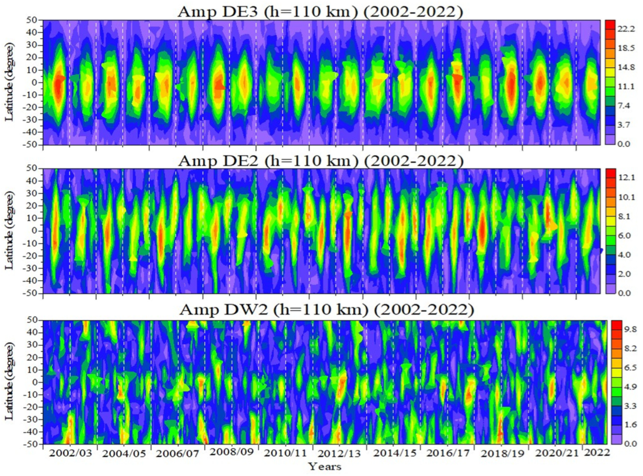
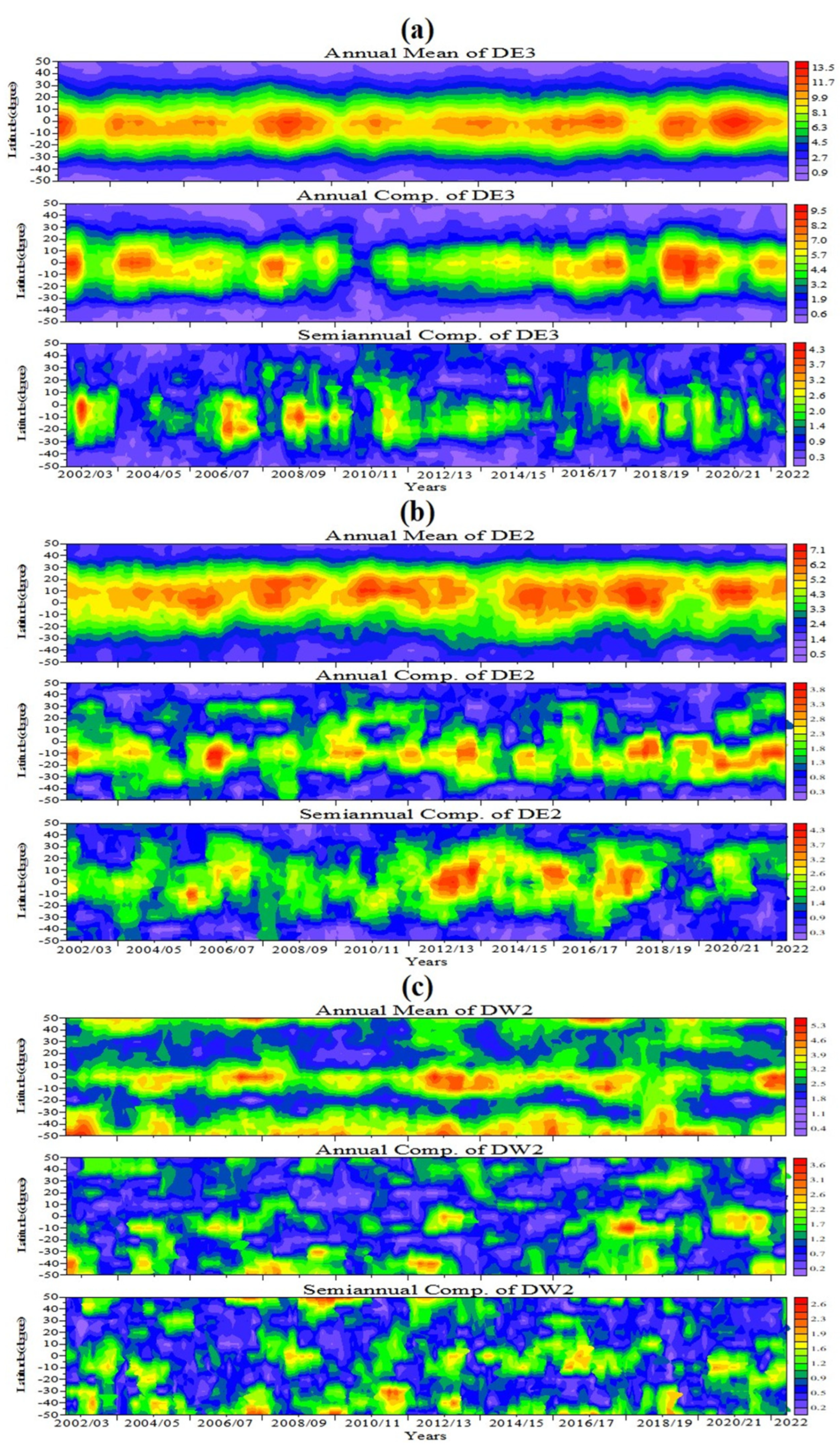
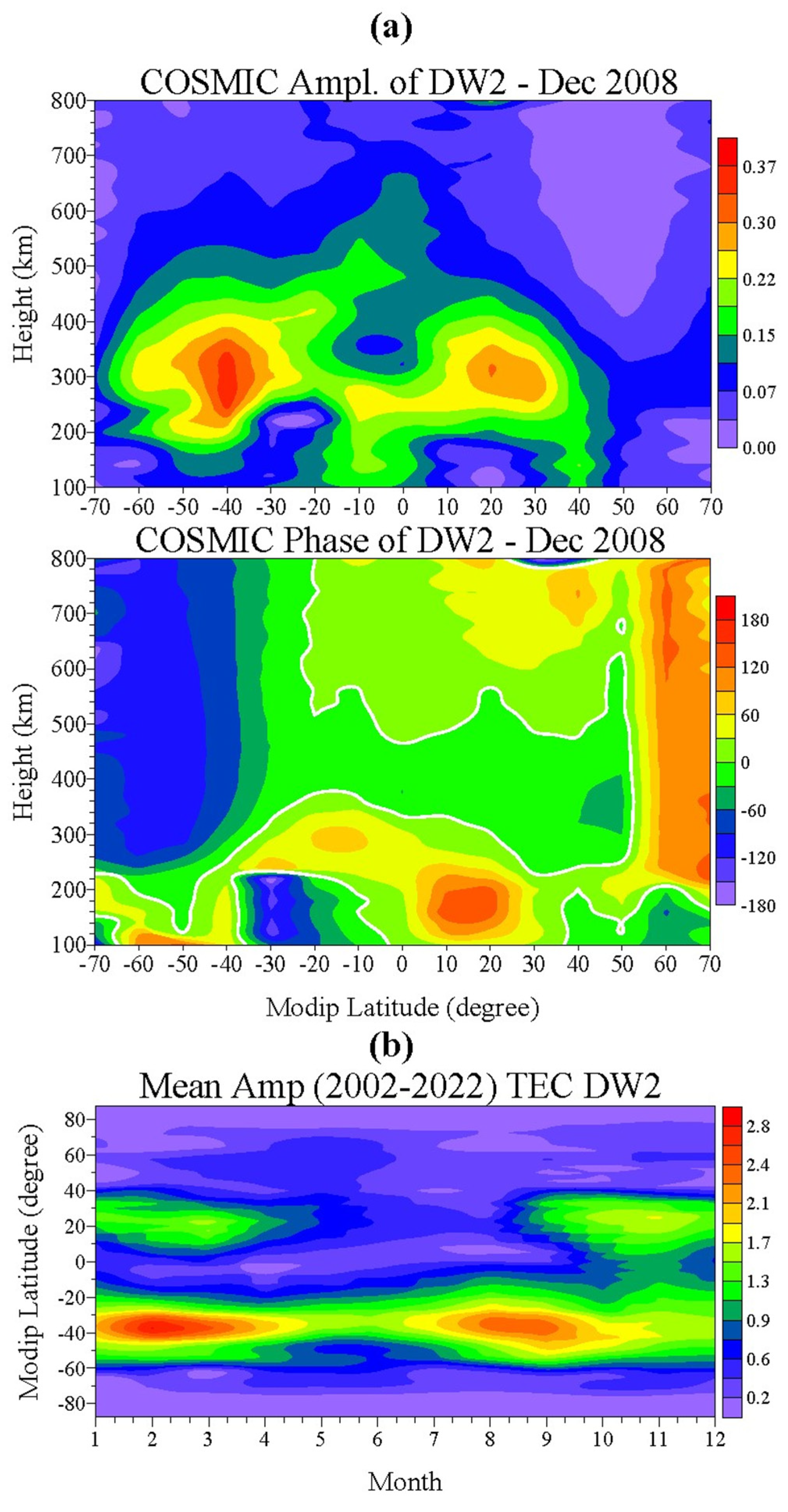
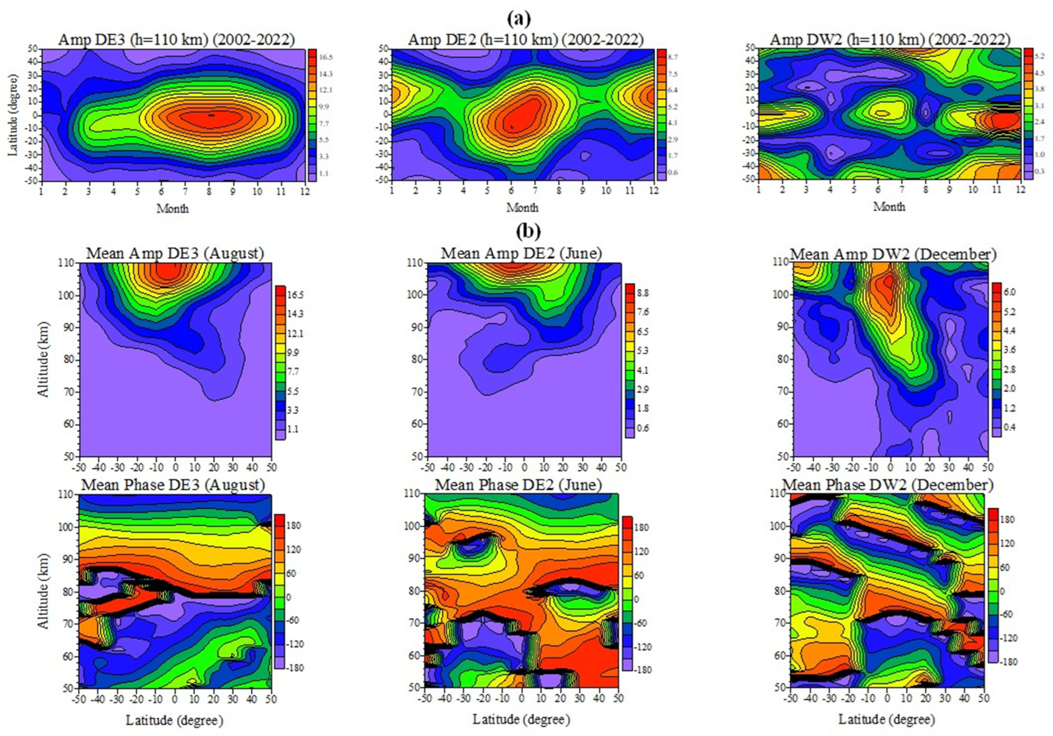
3.1. Climatology, Seasonal and Interannual Variability of the Nonmigrating Diurnal Tides

It is worth noting that the considered nonmigrating diurnal tides DE3 and DE2 are the first and second strongest tides, while DW2 is the fourth one among all diurnal tides for the entire period of 21 years; additionally, DE3 is the strongest nonmigrating tide among all such tides. Miyoshi et al., 2017 [11], clarified that the excitation source of DE3 is the latent heat release associated with the largest wavenumber 4 component of the cumulus convection (because the zonal wavenumber 4 component is the largest in the land–sea distribution at low latitudes, [78] while DE2 is considered to be excited by the cumulus convective activity with zonal wavenumber 3 in the troposphere). Pancheva et al., 2009 [6], showed that the enhancement of DW2 amplitude occurs during a sudden stratospheric warming (SSW) event in the NH, i.e., the source of DW2 is the nonlinear interaction between the SPW1 and the migrating DW1 tide. Later, Niu et al., 2018 [79], examined the relationship between SPW1 and DW2 waves for 31 winters from 1979 to 2010, with the extended Canadian Middle Atmosphere Model (eCMAM) through correlation and composite analysis. The authors found that although SPW1 is usually very strong during SSW events, especially with displacement, this, however, does not warrant a stronger interaction with DW2. Some evidence that the winter SSW events lead to the generation of DW2 can be found out in the secondary winter maxima at both hemispheres in the climatology of this tide (Figure 1). Additionally, Hagan and Forbes, 2002 [8], by using the GSWM, showed that DW2 is excited by the cumulus convective activity with zonal wavenumber 1, and it has considerable amplitudes in the MLT region. Furthermore, Pancheva et al., 2014 [31], revealed that the DW2 tidal variability of the MLT follows El-Ninõ–Southern-Oscillation variability, suggesting the importance of interannual variability of cumulus convection in the tropics. Thus, the excitation source of DW2 is not yet clear, and it would be a subject for future study [11].
Figure 1a shows the climatologically mean (2002–2022) latitude-time structures of the DE3 (left plot), DE2 (middle plot), and DW2 (right plot) tidal amplitude (in Kelvin) calculated at altitude of 110 km. It is important to underline that in the present study, all figures will use different color scales for the tides under consideration; this makes it possible to immediately assess the climatologically or monthly mean magnitudes of the tidal amplitude. The DE3 and DE2 tides have been investigated by many authors, and regardless of the different time intervals used, the climatological characteristics of these two tides remained almost unchanged. For example, the largest mean (for full 21 years) tidal DE3 (DE2) amplitude, observed in August–September (June), is ~16.5 K (~8.7 K) while that of the secondary amplification in March–April (December) is about 9 K (~8 K). According to Pancheva et al., 2010 [27], only for 6 full years (2002–2007) are the main and secondary maxima for both tides are observed in the same months with the respective mean amplitudes of ~15 K (~8.3 K) and ~8 K (~8 K). The DE3 is symmetrical tide about the equator, while June DE2 maximum is located at ~10° S, and that in December is at ~10° N. The climatology of DW2 reveals enhancements around the equator, and at ±50° with the largest amplitudes in November (~5.2 k) at the equator, in August (~4.5 K) at 50° N, and in December (~4.8 k) at (40–50°) S. Figure 1b demonstrates the altitude-latitude structures of the tidal amplitudes (upper row of plots, in K) and phases (bottom row of plots, in degrees) of the above-mentioned diurnal tides arranged in the same way as in Figure 1a; DE3 is presented in August, while DE2 and DW2 are presented in June and December, respectively. All these tides are vertically upward-propagating and reach the largest amplitudes at or slightly above 110 km height, with an exception of DW2 tide over the equator, particularly in December, which maximizes around 105 km with amplitude of 6 K.
The next step in our analysis is to look at the distribution of the monthly mean tidal amplitudes of the above considered nonmigrating diurnal tides. Figure 2 presents the latitude-time structures of the monthly mean DE3 (upper plot), DE2 (middle plot), and DW2 (bottom plot) tidal amplitudes at altitude of 110 km; the time is actually the number of months started from January 2002. It is seen that during the considered period of 21 years the monthly mean DE3 tidal amplitude reaches 22.2 K, while those of DE2 and DW2 are, respectively, 12.1 K and 9.8 K, i.e., these nonmigrating tides have a large contribution to the neutral dynamics of the lower thermosphere. Furthermore, the monthly mean representation shown in Figure 2 allows for both the highlighting of the main seasonal components and the rapid visualization of the interannual variations if they exist. It can be distinguished that for DE3 tide, the main seasonal component is the annual one, while for DE2 and DW2 there is also a well-seen semi-annual component. Moreover, for DE2, the semi-annual component is better delineated than the annual component, while in some years for DW2, a 4-month component can also be distinguished. Figure 2 reveals very clearly the presence of interannual variations in all considered tides. The quasi-2-year variability can be noticed at once in DE3 and DE2, particularly in the June maximum; some signature of this variability can be distinguished in DW2 as well, especially in the December maximum at southern middle latitudes. The results in Figure 2 demonstrate that it is necessary to investigate in detail the seasonal components of the considered nonmigrating tides in the low thermosphere. The reason is that it is in the seasonal components that the interannual variability is best manifested, and this will be done as a next step of the tidal analysis.
Usually, the seasonal variability is described by the 12- and 6-month components, i.e., AC and SAC, but in this study, the shorter 4- and 3-month components are also included. Besides the above-mentioned seasonal components, an important parameter is the annual mean (AM) as well. All these components are separated from the monthly mean tidal amplitudes by a decomposition applied to a 12-month window that is moved through the time series with a step of 1 month in order to derive the monthly values of the seasonal characteristics. A careful inspection of the decomposition results indicated that the 4- and 3-month components are quite weak in comparison with the AC and SAC ones, so they will no longer be considered. Figure 3a shows the latitude-time structures of the AM (upper plot), AC (middle plot), and SAC (bottom plot) separated from the monthly mean DE3 amplitudes at an altitude of 110 km, while Figure 3b,c presents the same as Figure 3a, but for DE2 and DW2, respectively.
Figure 3a reveals quite large AM and AC of DE3 amplitudes reaching ~13.5 K and ~9.5 K. Both seasonal components are centered over the equator having large amplitudes between latitudes of ±10°. The quasi-2-year variability of these seasonal components can be well distinguished. The SAC of DE3 is significantly weaker than that of AC with the largest amplitude of ~4.3 K. It is seen that this component is distributed between latitudes of ±30°; it demonstrates some quasi-2-year variability, but there is also another, longer-term one. Considering the main seasonal component of DE2 (Figure 3b), it is right away evident that the SAC (4.3 K) is larger than the AC (3.8 K) one, i.e., a feature that was noticed from Figure 2 (middle plot) and mentioned above. The AM (7.1 K) of DE2 has maxima located between 15° N and 10° S depending on which solstice (June or December) maximum has the largest amplitude at the given month. During most of the time, the AC of DE2 is distributed between 10° N and 20° S, while the SAC is between ±20°. The quasi-2-year variability is best seen in AM, but can also be noticed in the other two seasonal components of DE2. Figure 3c presents the main seasonal components of DW2. According to the climatology of this tide (Figure 1) the seasonal components are also located over the equator and around ±50°. Considering the AM (5.3 k) of DW2, there is a better synchrony between the enhancements above the equator and those around 50° N than with those in the SH.
The use of the full 21 years of observations to investigate some nonmigrating tides at lower thermosphere provides an opportunity to examine their interannual variations. It is known that the 11-year solar cycle (SC) and the quasi-biennial oscillation (QBO) has long been observed to be globally prevalent, as the QBO impact, particularly at low and low-middle latitudes, is a predominant one [80,81]. The QBO is the dominant signal in the stratosphere, and although it is a tropical phenomenon, it modulates the stratospheric flow from pole to pole [82].
The solar radio flux index F10.7 is used as a proxy of solar activity, and the monthly mean data were downloaded from the website: https://omniweb.gsfc.nasa.gov/ow.html (accessed on 9 April 2024). The QBO index at 30 hPa is obtained from https://www.cpc.ncep.noaa.gov/data/indices/ (accessed on 10 April 2024). The SC and QBO impact on the seasonal components of the considered DE3, DE2, and DW2 tides will be investigated using across-correlation analysis between the monthly mean F10.7 index and QBO data and the respective monthly mean seasonal components presented in Figure 3.
Figure 4a (left column of plots) presents the cross correlation functions between the QBO at 30 hPa and the AM (upper plot), AC (middle plot) and SAC (bottom plot) of the DE3, while Figure 4b (middle column of plots) and 4c (right column of plots) show the same as Figure 4a, but for DE2 and DW2. We underline that only the cross-correlation function at latitudes where the respective seasonal components have large amplitudes makes physical sense. A strong positive correlation of 0.7 between the QBO and the AM of DE3 (near the equator) is immediately apparent in Figure 4a, as the AM of DE3 lags behind the QBO with a month. The other two seasonal components of the DE3 also reveal positive correlation with smaller coefficients, respectively 0.35 for the AC and 0.45 for the SAC, but with longer delay, ~2–3 months for the AC and ~6 months for the SAC, respectively. It is worth noting that the quasi-2-year variability of the DE3 in the MLT region has been investigated with simulations with the GAIA model [11]; the authors reported that it is generated by quasi-2-year variation in the zonal mean zonal wind between 40 and 70 km, which is modulated by the stratospheric QBO.
The seasonal components AM and AC of DE2, however, demonstrate a negative correlation (Figure 4b), −0.6 for the AM and −0.4, respectively, for the AC, as both components lag behind the QBO with ~6 and ~8–9 months. It has been mentioned above that the SAC of DE2 is located between latitudes of ±20°. The bottom plot of Figure 4b shows positive correlation between the QBO and the SAC of DE2 at 20° N, 0.45, and a weaker negative one, −0.20, at 20° S; both maxima lag behind the QBO with 6–8 months. We consider that the QBO variability of the DE3 and DE2 tides studied by Pancheva et al., 2010 [27], applying a different approach on only a 6-year interval (2002–2007), indicated that this dependence was well evident. The cross-correlation between the QBO and the seasonal components of DW4 (Figure 4c) is weaker in comparison with those of DE3 and DE2. While the AM around the equator shows a negative correlation of −0.4 with a time lag of ~2 months, those at ±(40–50°) are out of phase with the QBO. Similar but weaker correlations are seen for the AC and SAC near the equator, as well as with longer time lags, ~7–9 months.
In summary, the seasonal components of the considered DE3, DE2, and DW2 tides in the lower thermosphere demonstrate quite significant QBO variability, particularly the DE3 tide; its AM seasonal component near the equator demonstrated a positive correlation of 0.7, with a month lag behind the QBO index at 30 hPa.

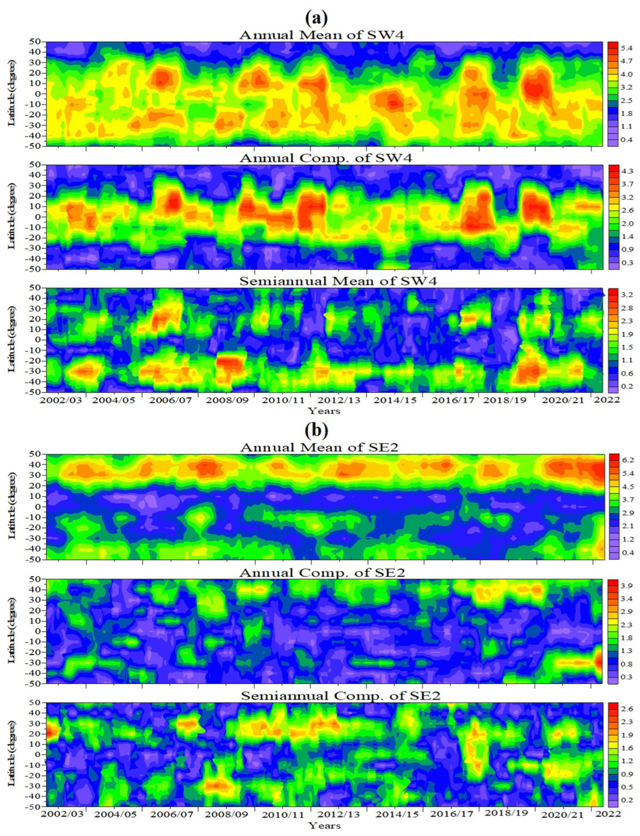
3.2. Climatology, Seasonal and Interannual Variability of the Nonmigrating Semidiurnal Tides

The main features of the nonmigrating SW4 and SE2 tides will be presented by following the same pattern as that for the diurnal nonmigrating tides. These tides are actually the second and third strongest tides among all semidiurnal nonmigrating tides for the entire period of 21 years. Just for information, we will note that the strongest semidiurnal nonmigrating tide for the considered 21 years is the SW3 with climatologically mean amplitude slightly larger than 9 K. While the most probable excitation source of SW4 is the nonlinear interaction between the SPW2 and the migrating SW2 tide, that of the SE2 is the latent heat release associated with the 12 h variation in cumulus convection with zonal wavenumber 4 [11]. However, Hagan et al., 2009 [83], and to some degree verified by Oberheide et al., 2011 [28], reported that the nonlinear interaction between DE3 and DW1 can also produce SE2.
Figure 5a shows the climatologically mean (2002–2022) latitude-time structures of the SW4 (left plot) and the SE2 (right plot) tidal amplitudes (in Kelvin) calculated at altitude of 110 km. It is seen that the climatologically mean amplitudes of both tides are very close, 6.7 K for SW4 and 6.6 K for SE2. Truskowski et al., 2014 [84], investigated the above-considered tides for 9 years (2002–2010), finding very similar to Figure 5a latitude-time structures at altitude of 110 km with the same for the two tides largest amplitudes of 6.4 K. Furthermore, the SE2 tide was studied by Pancheva et al., 2010 [27], for only six full years (2002–2007) and the authors also obtained similar latitude structure to that in Figure 6a, with the largest amplitude of ~6 K. Figure 6b presents the altitude-latitude structures of the tidal amplitudes (upper row of plots, in K) and phases (bottom row of plots, in degrees) of the above-mentioned semidiurnal tides arranged in the same way as in Figure 1a; SW4 is shown in February, while SE2 is shown in May. Both tides are vertically upward-propagating, and most probably reaching the largest amplitudes slightly above 110 km height.
Figure 6 presents the latitude-time structures of the monthly mean SW4 (upper plot) and SE2 (bottom plot) tidal amplitudes at altitude of 110 km; the time, again, is the number of months started from January 2002. It is seen that, during the considered period of 21 years, the monthly mean SW4 tidal amplitude reaches 10.5 K, while that of SE2 is 8.9 K or these nonmigrating tides also have large contribution to the neutral dynamics of the lower thermosphere. Regarding the highlighting of the main seasonal components, it can be noticed that the SW4 in the NH reveals mainly AC, while in the SH, the SAC can be well-visible as well; a similar feature is seen for the SE2, i.e., the AC in the NH is larger than that in the SH. Figure 6 reveals the presence of interannual variations as well, and it is more evident in SW4, particularly around latitudes of 0–15° N.
Figure 7a demonstrates quite large AM of SW4 amplitudes reaching ~5.4 K; it is distributed between 30° N and 40° S, but the main AM amplitudes are centered at 15° N, over the equator and around 30° S. The largest amplitudes of the AC and SAC of SW4 are, respectively, 4.3 K and 3.2 K; while the distribution of the AC is located between ±20°, that of the SAC is centered around 20° N and 30° S. Considering the main seasonal components of SE2 (Figure 7b), it is right away evident that the AM (6.2 K), particularly in the NH, is significantly larger than the AC (3.9 K) and SAC (2.6 K) ones. While the AM in the NH is centered around (30–40°) N, that in the SH is at a latitude of ~40° S. Generally, the NH AC, centered at ~40° N, is stronger than that in SH located around (30–40°) S. The SAC also shows some hemispheric asymmetry, but weaker than those of the AM and AC; while the NH SAC is centered around (20–30°) N, the SH SAC can be seen between 20° S and 40° S. Some interannual variability, mainly the quasi-2-year one, can be distinguished mainly in the AM and AC of SW4 and in the AM, particularly in the NH of SE2.
Figure 8a (left column of plots) presents the cross-correlation functions between the QBO at 30 hPa and the AM (upper plot), AC (middle plot), and SAC (bottom plot) of the SW4, while Figure 8b (right column of plots) shows the same as Figure 8a, but for SE2. We again underline that only the cross-correlation function at latitudes where the respective seasonal components have large amplitudes makes physical sense. A quite strong positive correlation of 0.5 between the QBO and the AM of SW4 (near the equator) is evident in Figure 8a (upper plot); that is, however, out of phase with the stratospheric QBO. There is also a weaker positive correlation of ~0.30 near 20° N that lags behind of the QBO with 9–10 months. The AC of SW4 (middle plot) at (10–20°) N also demonstrates strong positive correlation of 0.55 with a time delay of 8–9 months. A positive correlation of 0.40 shows the SAC of SW4 (bottom plot) at ~20° S, with a time delay of 6–7 months. The AM seasonal component of SE2 around (30–40°) N demonstrates a negative correlation of −0.50 (Figure 8b, upper plot) with a time lag of ~7 months; negative correlations also show at the AM at ~10° S and 40° S, with a shorter time lag of ~2–4 months. The AC of SE2 (middle plot) is strong at (30–40°) N, but there is a negative maximum of only −0.30 around 30° N that is out of phase with the QBO. The AC of SE2 in the SH is significantly weaker than that in the NH; however, it reveals a positive correlation of ~0.30 around (30–40°) N that also is out of phase with the QBO. The SAC of SE2 (bottom plot) at latitude of ~20° N reveals a weak positive correlation of ~0.25 and out of phase dependence with the stratospheric QBO; there is stronger correlation of 0.35 of the SAC at around 10° S, but there this component is not large.
Summarizing the interannual variability of the SW4 and SE2 seasonal components, we may conclude that, similarly to the considered diurnal nonmigrating tides, here, also, it demonstrates well-visible QBO variability in the lower thermosphere. In general, the QBO impact is weaker than that on the considered diurnal nonmigrating tides.
Finally, it is worth mentioning that we also considered the solar cycle (SC) influence of the here-investigated diurnal and semidiurnal nonmigrating tides, again by using cross correlation analysis. The results, however, indicate that, in general, the SC effect on these tides is weak.

4. Climatology (2002–2022) of Longitudinal Structures in the Lower Thermosphere

It has been already mentioned that, based on the observations made by the SABER and TIDI instruments on the TIMED satellite, even the first climatologies of the most important tidal components in temperature and neutral winds [20,22,27,85] revealed an important result that nonmigrating tides are much larger than hitherto anticipated, and some of them often exceed their migrating counterparts. The nonmigrating tide that has so far attracted most attention is DE3 because it is the largest component during most of the year. The presented in this study climatology based on very long term observations (2002–2022) fully confirms previous climatological reports obtained on much shorter observations. It is important to note that the E3 appears as a zonal wavenumber 4 (wave-4 or WN4) longitudinal structure in the lower thermosphere when observed at constant LT. We consider that Miyoshi et al., 2017 [11], clarified that the excitation source of DE3 is the latent heat release associated with the largest wavenumber 4 component of the cumulus convection in the troposphere; hence, the coupling between the troposphere and lower thermosphere is carried out through this nonmigrating tide. Similarly to the DE3, the DE2 appears as a zonal wavenumber 3 (wave-3 or WN3) longitudinal structure in the lower thermosphere at constant LT. Therefore, these nonmigrating tides, as well as other large nonmigrating ones, can generate longitude structures when they are observed at constant LT [28,50].
To understand why the nonmigrating tides can produce different longitudinal structures, let us consider the main difference between the migrating and nonmigrating tides. In general, the atmospheric tides can be expressed generally in the form:
Cks cos [k(2π/24)t − sλ − γks]
where t is universal time in hours, λ = longitude, k = number of the diurnal harmonic, γks = tidal phase, and s is zonal wavenumber; the latter is positive when the tide propagates eastward, it is negative at westward propagation and s = 0 at zonally symmetric (or standing) tide. It has been mentioned before that the longitudinal structures are seen at fixed local time. If the general tidal expression (1) is converted from universal time to a local time frame by having in mind that t = tLT − 24/2π, then we get:
Cks cos [k(2π/24)tLT − (k + s)λ − γks]
Migrating tides propagate westward (s < 0) with the apparent motion of the Sun, and are thus Sun-synchronous and longitude-independent when observed at constant local time. This means that the zonal wavenumber, s, is equal to the number of the diurnal harmonics, k, but has a negative sign. Therefore k + s = 0 indicating that the migrating tides are longitudinally independent. Nonmigrating tides are excited by zonally asymmetries (i.e., longitudinally dependent absorbing species) hence, they are longitudinally dependent and their zonal wavenumber, s, is not equal to the number of the diurnal harmonics, k, i.e., k + s ≠ 0. The expression (2) indicates that an observed longitudinal structure in satellite data cannot be related unambiguously to a certain tidal component because it is consistent with any values of s and k for which holds |s + k| is equal to the corresponding structure number. First, WN4 and WN3 longitudinal structures in the lower thermosphere have been reported by Oberheide and Forbes, 2008 [86]. For this purpose, the authors used SABER temperature data from 2002–2006 and the nitric oxide density measured from the Student Nitric Oxide Explorer (SNOE) satellite [87] for the period of 11 March 1998–30 September 2000, i.e., for a full 2.5 years. The authors found that in the altitude range of ~105–110 km where the NO has maximum, the WN4-like signature between March and October is produced by DE3, while the WN3-like signature in December and January is introduced by DE2 and SE1. This study revealed the large influence of nonmigrating tides on the NO variability in the lower thermosphere regardless of the fact that the SABER/TIMED and SNOE observations represent different time intervals; hence, the NO density is used as a tracer of the nonmigrating tidal dynamics. In a similar way, Pancheva et al., 2014, demonstrated that the mesospheric ozone derived from the SABER/TIMED is a tracer of the nonmigrating tides DE3, DW2, and SW3 [31]. The DE3 modulation of the EEJ is also an example of the presence of the WN4 structure registered in the lower thermosphere [45,46].
The above-mentioned examples of the observed longitudinal structures in the lower thermosphere show quite limited time intervals of observations. Additionally, usually these structures and especially the WN4 one is connected only with the DE3, but this is not always the case. It is known that besides DE3 and DE2 responsible mainly for the WN4 and WN3 structures other nonmigrating tides, and SPWs are involved in their formation. The basic aim of this section is to present evidence for the existence of longitudinal structures in the lower thermosphere based on large statistics. The formation of these structures will include all those nonmigrating tides and SPWs which contribute to the formation of these structures, except the quarterdiurnal ones, which are very weak.

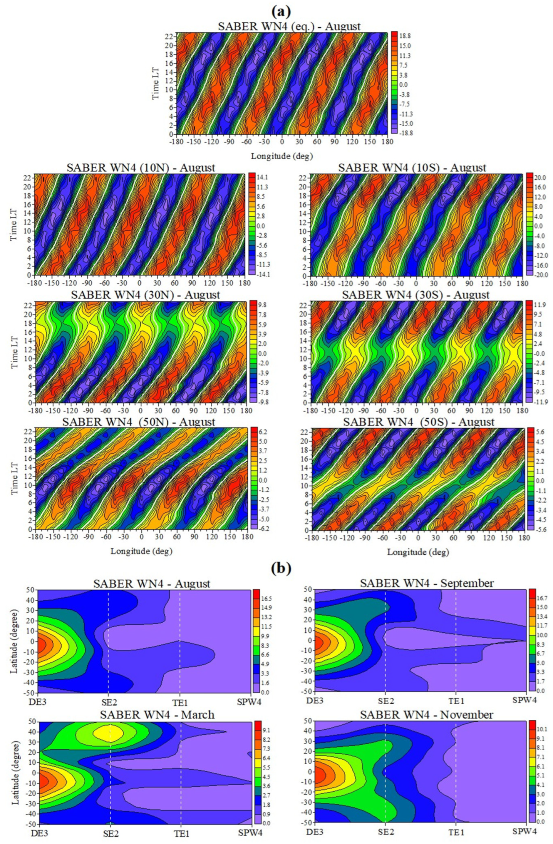
4.1. SABER Temperature WN4 Structure

In the context of the method applied in the present study for separating the tides from the SABER temperatures, described in detail by Pancheva and Mukhtarov, 2023 [71], and the expression (2), in our case, k = 1, 2, 3, 4 while s changes from −4 to +4. The WN4 structure can be determined by |s + k|= 4. If the quarterdiurnal nonmigrating tides are excluded, then the WN4 structure can be generated by DE3, SE2, TE1 (T is for terdiurnal), and SPW4.
Figure 9a shows the LT variability of the climatologically mean (2002–2022) SABER WN4 structure in August at different latitudes (they can be seen in the upper side of each plot); the uppermost plot reveals the structure over the equator, while the left and right column of plots demonstrates the NH and SH, respectively. We clarify that the climatologically mean WN4 structure signifies the superposition of the climatologically mean DE3 + SE2 + TE1 + SPW4. Figure 9a produces the WN4 structures at different latitudes only in August, not only because then the WN4 has the largest amplitudes (not at all latitudes), but also because such presentation provides the opportunity to trace how the LT dependence changes with the latitude, and also to shed a light on the hemispheric asymmetry during this month. The main features of the WN4 structure in the lower thermosphere (altitude of 110 km) can be summarized as: (i) in the latitudes of (0–10°) S the largest amplitudes of the WN4 structure (respectively 18.8 K and 20 K) are stronger than that of the DE3 (16.5 K, Figure 1); (ii) while at low and partly tropical latitudes, the WN4 structures show more than one enhancement at middle latitudes, and there is only one amplification; the observed enhancements reveal clear latitude dependence; (iii) at latitudes of ±30° the WN4 structure almost disappears around 18 LT at 30° N and 11 LT at 30° S; this could be related to changes of the tidal contribution (for example, some decrease in the SE2 contribution); and (iv) while the WN4 structures at latitudes of (10–30°) S are stronger than those at (10–30°) N, at middle latitude (±50°) the opposite dependence is seen.
It is worth noting that in the latitude bands of (10–30°) N(S), the largest WN4 amplitudes are observed in September (August), while in those of (40–50°) N(S) in March (November). Furthermore, considering the largest WN4 structures at all latitudes and months, the above-mentioned hemispheric asymmetry is still valid. We have made an attempt to assess the contribution of each nonmigrating tide and SPW4 during the months when the WN4 structure is strong. Figure 9b presents the latitudinal dependence of the tidal and SPW4 contribution to the WN4 structure in the months when it has large amplitudes; these are August (upper left plot), September (upper right plot), March (bottom left plot), and November (bottom right plot). These results confirm the already known features that the DE3 has the largest contribution to the WN4 followed by the SE2; the latter contributes the most in March and September, with a stronger contribution to the NH (we consider that the largest SE2 amplitude is observed at ~40° N, Figure 5) than that to the SH. The third contributor is the TE1, while the SPW4 is the weakest one.

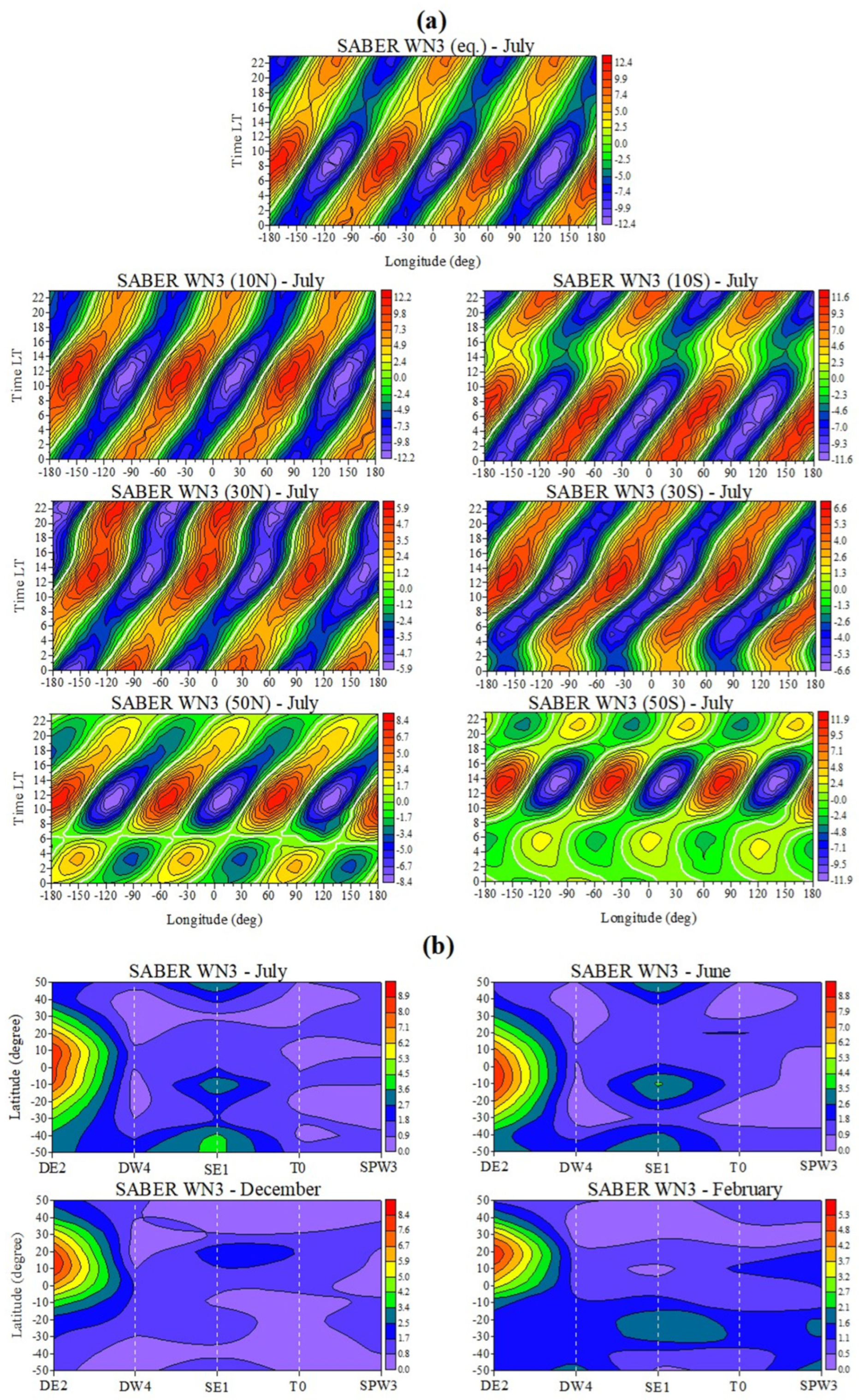
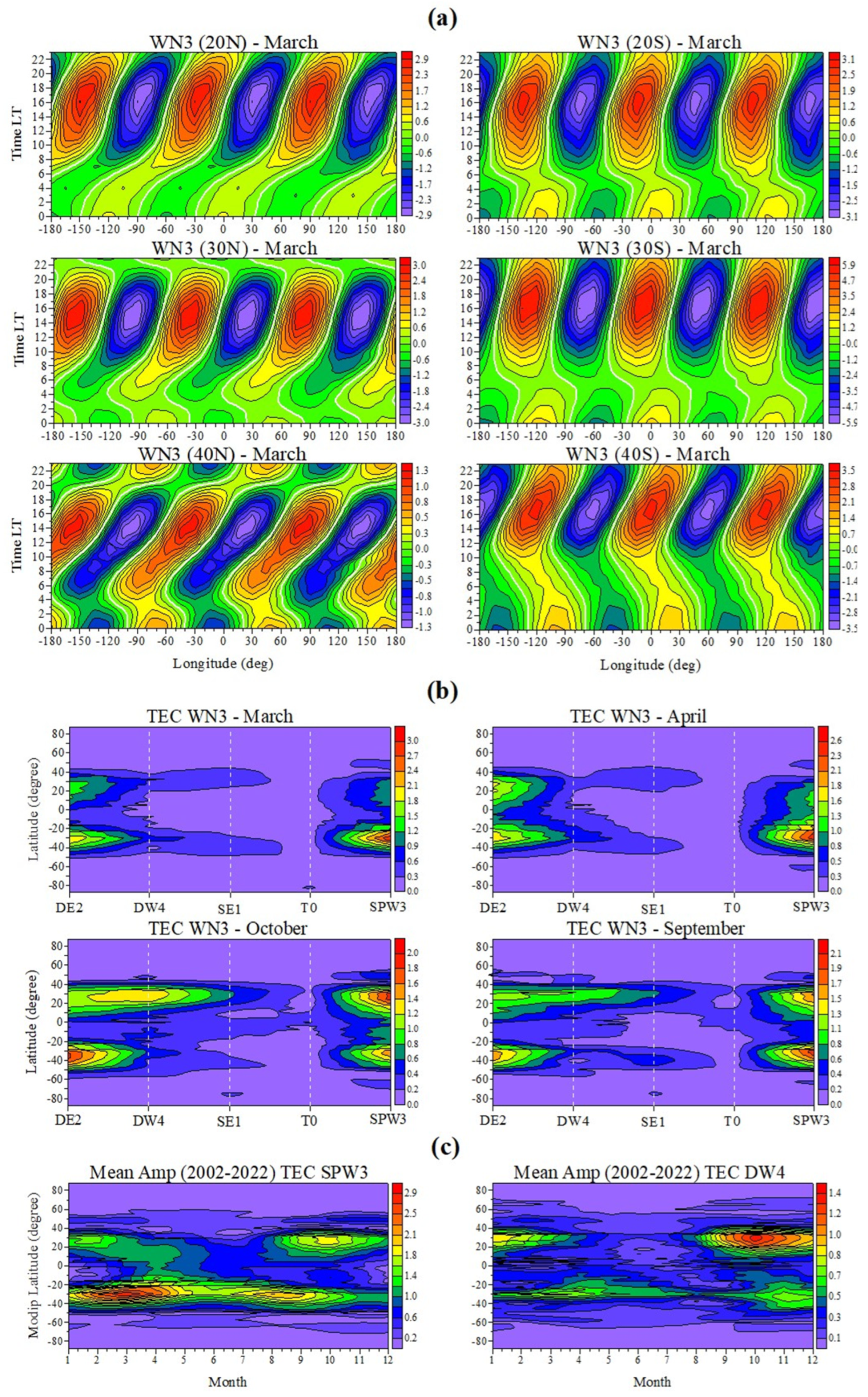
4.2. SABER Temperature WN3 Structure

The WN3 structure in the lower thermosphere, besides DE2, can also be generated by DW4, SE1, T0, and SPW3 (based on |s + k| = 3).
Figure 10a shows the LT variability of the climatologically mean (2002–2022) SABER WN3 structure in July at different latitudes; the plots are arranged in the same way as those in Figure 11a. Again, the climatologically mean WN3 structure denotes the superposition of the climatologically means DE2 + DW4 + SE1 + T0 + SPW3. The main features of the WN3 structure in the lower thermosphere (altitude of 110 km) and in July can be summarized as: (i) the WN3 structures at latitudes of ±10° and 50° S is stronger than the climatological mean of the DE2 at altitude of 110 km (8.7 K, Figure 1); (ii) at all latitudes the WN3 structures reveal one main enhancement during the daytime and a secondary one in the late evening or early morning hours; (iii) the daytime maxima fluctuate between 11 LT and 13 LT with the latitude in the NH, while in the SH the fluctuation range is larger, between ~8 LT and 13 LT.; (iv) at 50° N, the evening WN3 disappears, while at 50° S it is very weak; and (v) this structure does not show clear hemispheric asymmetry in July.
Considering the largest WN3 structures at all latitudes and months, it worth noting that: at latitudes of 0–10° N and at ±(40–50°), the strongest WN3 is observed in July, while at (10–20°) S it is in June, at (20–30°) N it is in December, and at 30° S it is in February. This is the reason Figure 10b shows the latitudinal dependence of the tidal and SPW3 contribution to the WN3 structure in the months when it has large amplitudes these are July (upper left plot), June (upper right plot), December (bottom left plot), and February (bottom right plot). These results also confirm the already known features that the DE2 has the largest contribution to the WN3 followed by the SE1; the latter contributes mostly in July and June at latitudes of ±50° and at ~10° S, i.e., exactly when and where the SE1 has the largest climatologically mean amplitudes at an altitude of 110 km. The third contributor is the SPW3, while the T0 and DW4 are the weakest ones.

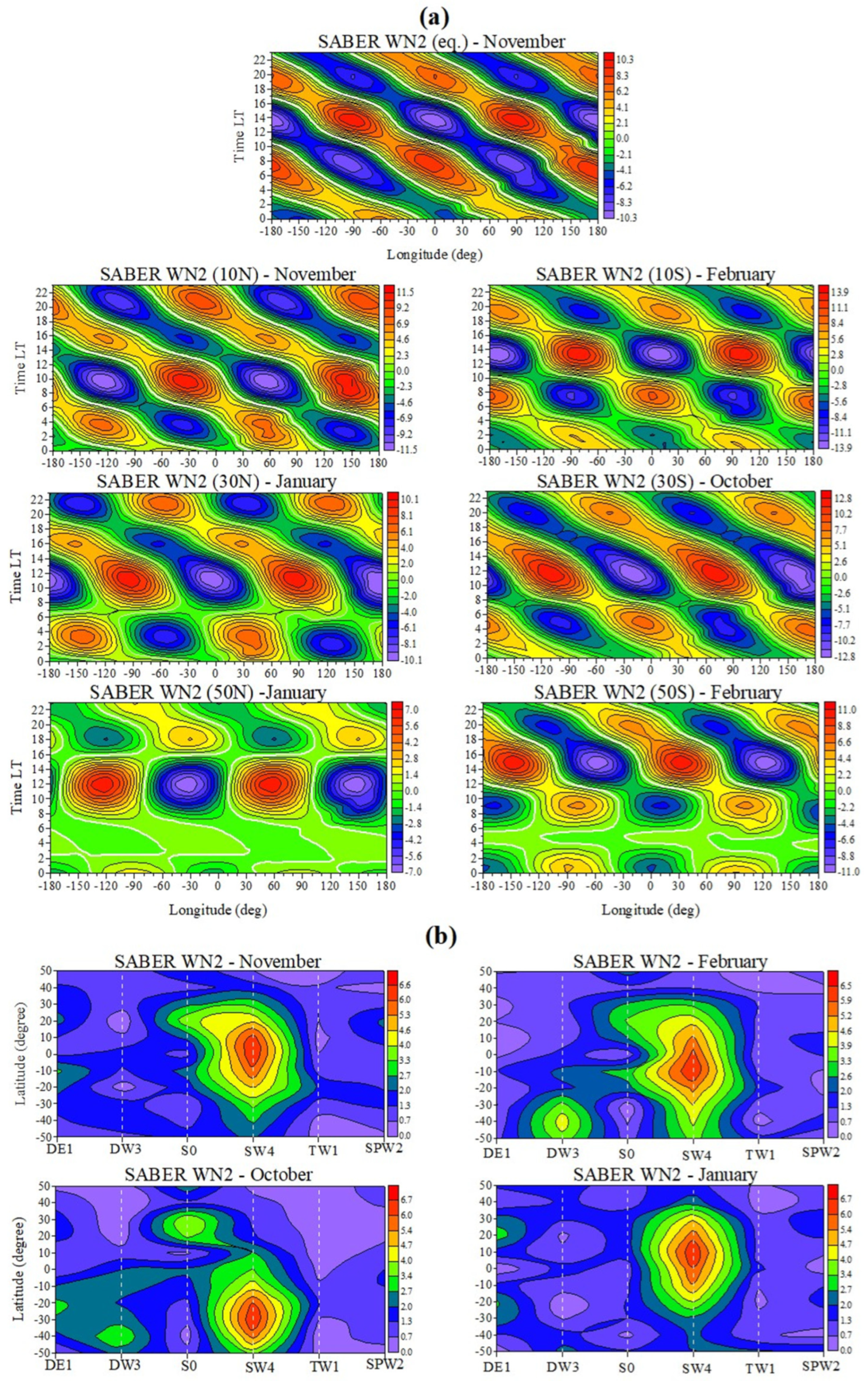
4.3. SABER Temperature WN2 Structure

According to the authors’ knowledge, the WN2 longitudinal structure has not been seriously investigated in the lower thermosphere. Only very recently, based on the neutral wind observations from the Michelson Interferometer for Global High resolution Thermospheric Imaging (MIGHTI) instrument onboard Ionospheric CONnections (ICON), Li et al., 2023, have studied the longitudinal structures from WN1 to WN4 in the zonal wind [88]. The ICON/MIGHTI zonal wind from version V04 data from December 2019 to January 2022 (about 2 years) were used during the daytime, when the neutral wind data can cover the altitude range of 100–300 km by combining the winds of the red line and green line. Actually, the authors did not report any clear features of the WN2 structure in the IT system, mentioning only that “the main wave sources of WN1 and WN2 have complex variations with altitude, latitude, and season”.
The present climatological study of the nonmigrating tides based on large statics provides an excellent opportunity for the first time the WN2 longitudinal temperature structure in the lower thermosphere to be examined in detail. The WN2 structure in the lower thermosphere can be generated by DE1, DW3, S0, SW4, TW1, and SPW2 based on |s + k| = 2. The preliminary inspections of the WN2 structure revealed that this structure is strong predominantly during winter months. Figure 11a shows the LT variability of the climatologically mean (2002–2022) SABER WN2 structure at different latitudes and in different winter months; the latter are shown in the upper side of each plot. Similarly to the previous two cases here also the climatologically mean WN2 structure denotes the superposition of the climatologically means DE1 + DW3 + S0 + SW4 + TW1 + SPW2. The main features of the WN2 structure in the lower thermosphere (altitude of 110 km) can be summarized as: (i) unlike the WN4 and WN3 structures, which slope to the east, this WN2 structure slopes to the west; this is most likely due to the predominant influence of the nonmigrating tides propagating westward; (ii) the WN2 structure reveals clear hemispheric asymmetry as it is stronger in the SH than that in the NH; the largest magnitude of the WN2 reaches ~13.9 K at latitude of 10° S making it stronger structure than the WN3 one in the lower thermosphere; (iii) at all latitudes the WN2 structures reveal two or even three enhancements; the main maxima are located between 11–12 and ~15 LT; and (iv) at latitudes of ±50°, the WN2 structure almost disappears between 2–3 and 6–7 LT.
Figure 11b shows the latitudinal dependence of the tidal and SPW2 contribution to the WN2 structure in the winter months when this structure has large amplitudes, as these are November (upper left plot), February (upper right plot), October (bottom left plot), and January (bottom right plot). These results clearly indicated that the SW4 has the largest contribution to the WN2 followed by DW3, S0, DE1, and SPW2; the TW1 has the weakest contribution. The latitude structure of the SW4 contribution to large extend defines the seasonal dependence of the WN2, i.e., the month when the structure has the largest magnitude at a given latitude determined by the SW4; for example, in November, the SW4 maximum is located at ~10° N, in February it is at ~10° S, and in October it is at ~30° S. While this dependence can also be recognized to some extent at a latitude of 50° S in February where both tides SW4 and DW3 have not small amplitudes, it is not valid for January at a latitude of 50° N.
This section investigated in detail the climatological (2002–2022) features of the longitudinal WN4, WN3, and WN2 structures in the lower thermosphere (altitude of 110 km). The WN4 is the strongest structure with the largest magnitude of 20 K observed at 10° S in August. The WN4 has larger magnitude in the SH than that in the NH at latitude range of ±30°. The WN2 is the second strongest structure whose magnitude reaches up to ~13.9 K at latitudes of 10° S in February; this structure demonstrates clear hemispheric asymmetry, as the SH structure is stronger than the NH one at the entire latitudinal range (±50°). The WN3 is the weakest structure, with the largest magnitude of 12.4 K observed over the equator in July; this structure does not reveal clear hemispheric asymmetry.

5. Climatology (2002–2022) of Longitudinal Structures in the Ionosphere

We mentioned in the Introduction that with the advent of new satellite missions, recently there has been considerable interest in studying the coupling processes between the lower atmosphere and the IT system. Further, it was noted that the atmospheric tides, and particularly the nonmigrating ones, are the primary source for the ionosphere variability forced from below. The previous two sections of the present study clearly revealed that not only some nonmigrating tides, but also the longitudinal structures in LT they produced have large climatological (2002–2022) magnitudes in the lower thermosphere. There are quite many reports, mentioned in the Introduction, for the presence of such longitudinal structures, particularly the WN4 and WN3 ones, in the ionosphere as well.
Therefore, the next step in our analysis is to investigate the main climatological features of the longitudinal structures WN4, WN3, and WN2 in a way as they are present in the global TEC maps. The main reason is to quickly recognize these structures among the other ionospheric variations. This means that the absolute TEC magnitudes of the mentioned longitudinal structures will be considered. We underline that this is to some extent a weak point of the present paper because both the SC and semiannual variability of the TEC will not be removed in advance. However, we have to keep in mind that the TEC depends mainly on the electron density of the F-region maximum, but the bottom ionosphere has significantly weaker contribution than the topside one; this difference is considerable during night conditions. We note that although there are some already proposed methods to estimate the relative tidal amplitudes in the ionosphere [89,90], we would like to present a new approach for assessing the relative amplitudes and that will be the subject of a future study.
We remind that the TEC data: (i) cover the same time interval as that of the SABER temperature data, January 2002-Decemvber 2022; (ii) both the SABER temperatures and the TEC data are analyzed by using the same method, and (iii) while the SABER temperature results are presented in geographical coordinates those of the TEC are shown in modip latitude and geographic longitude. The longitudinal TEC structures are considered only at latitudes of ±50° not only because to compare them with the SABER temperature ones but also because at higher latitudes they quickly subside. Similarly to Section 4 here also the color scales at all latitudes will be different to distinguish right away the magnitude of the considered TEC longitudinal structure.

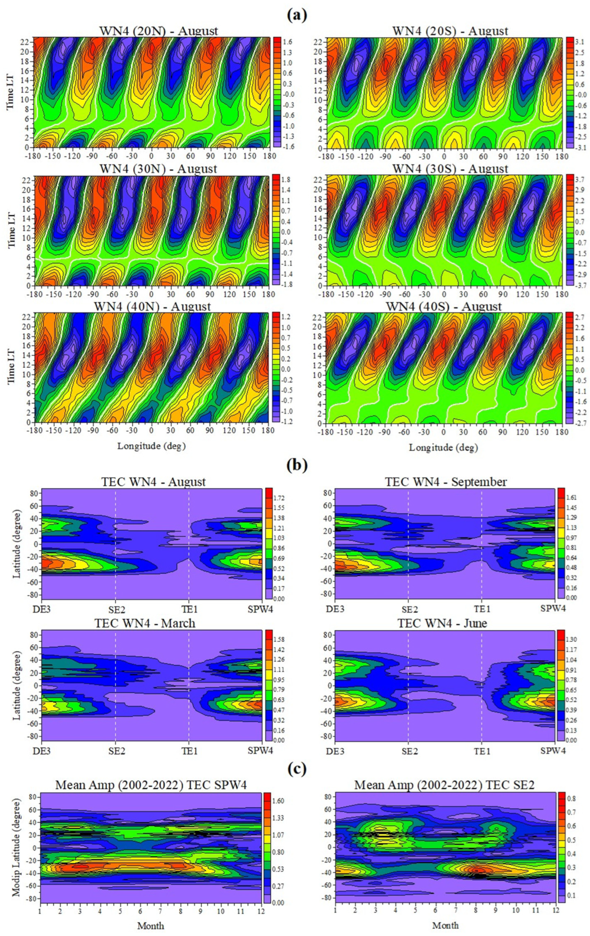
5.1. TEC WN4 Structure

The climatology of the TEC WN4 structure is calculated by the superposition of the same climatologically mean nonmigrating tides (and SPW4) as those in the lower thermosphere, i.e., DE3, SE2, and TE1. Figure 12a displays the LT variability of the climatologically mean (2002–2022) TEC WN4 structure at different latitudes, shown in the upper side of each plot, during August. Similarly to the climatology of WN4 in the lower thermosphere (Figure 9a) here, also, the largest magnitudes are seen in August and September. However, while in August, the WN4 largest magnitudes are seen at latitudes of ±(20–30°), and those in September are at latitudes of ±(40–50°). Keeping in mind that the EIA in modip latitude is located around ±30° then the largest WN4 structures occur in August, and this is the reason this month to be chosen for Figure 12a. The main features of the climatologically mean TEC WN4 structure can be summarized as: (i) although in this study we work with absolute tidal amplitudes, the seasonal dependence of the TEC WN4 structure is the same as that of the SABER temperature one in the lower thermosphere; this is mainly due to the similar seasonal variation of the SABER DE3 to the TEC semiannual one; (ii) there is a clear hemispheric asymmetry, as the SH structure (with the largest magnitude of 3.7 TECU) is stronger than the NH one (~1.8 TECU); this feature is similar to the SABER temperature one, but at latitudes of ±30°; (iii) at all latitudes, the WN4 structures disappeared or significantly weaken (as at 40° N) around 4–6 LT; this may be due to a change of the production mechanism; (iv) the strong WN4 structures are seen between 8–9 and 22–23 LT, and at all latitudes their maxima are centered around the longitudes: −180°, −90°, 0°, 90°, and 180°; and (v) there are WN4 structures between 00 and 04 LT as well, but their maxima are centered ~20–30° eastward of those observed during the daytime; these structures are stronger in the NH than those in the SH.
It is worth noting that besides August and September, large magnitudes are seen in June (over the equator) and May (at 10° N). Figure 12b presents the latitudinal dependence of the tidal and SPW4 contribution to the TEC WN4 structure in the months when it has large amplitudes; these are August (upper left plot), September (upper right plot), March (bottom left plot), and June (bottom right plot). These results confirm the already known features that the DE3 also has the largest contribution to the ionospheric WN4 structure, but in this case it is followed by the SPW4; the latter contributes the most in March and June. The third contributor is the SE2 while the TE1 is the weakest one. Figure 12c demonstrates the latitude-time climatological structure of the TEC SPW4 amplitude (left plot) and the TEC SE2 amplitude (right plot); both plots reveal clear hemispheric asymmetry, indicating that both waves SPW4 and SE2 are stronger in the SH. Keeping in mind that the same asymmetry exists in the DE3 electron density response at an altitude of 400 km [56] and in the TEC DE3 climatology in this study, the reason for the observed hemispheric WN4 asymmetry can be clarified.
According to Forbes et al., 2014 [91], the DE3 and SE2 are nonmigrating tides which can propagate from the lower thermosphere (110 km) up to the upper thermosphere at ~400 km. Pancheva and Mukhtarov, 2012 [55], show that the DE3 and SE2 responses in the F3/C electron density at altitude of 400 km. Hagan et al., 2007 [92] by using the GSWM with the TIME-GCM lower boundary (30 km) demonstrated that the DE3 could propagate from the troposphere into the lower thermosphere, modulate the E region dynamo process, and thereby introduce a four-peaked F region wave structure. Later, Hagan et al., 2009 [83], based on the simulations by the TIME-GCM, quantify, for the first time, the SPW4 in the MLT, and found that it is excited by nonlinear interaction between the DE3 and the migrating DW1; then the authors suggested that the SPW4 modulates the DE3 MLT response and may impact the E region dynamo as well as the ionospheric variability. Furthermore, Oberheide et al., 2011 [28], reported that the wave generation due the nonlinear interaction between the DW1 and the DE3 leads to a large SPW4 and a large SE2 tide in the E-region heights as their combined amplitudes can equal those of the DE3. Our climatology of the DE3, SPW4, and SE2 at altitude of 110 km, however, indicated that the DE3 (16.5 K) is significantly larger than the SPW4 (~2 K) + SE2 (~6.6 K) while in the thermosphere at 400 km the DE3 and SPW4 responses are not very different; the electron density DE3 response is 0.30 MHz and the SPW4 is 0.28 MHz [53] and the latter is supported by the present climatology, the TEC DE3 is 1.7 TECU and TEC SPW4 is 1.6 TECU. This could mean that the SPW4 is generated by the nonlinear interaction between DE3 and DW1, but in the IT system.

5.2. TEC WN3 Structure

In this sub-section, again the climatology of the TEC WN3 structure is calculated by the superposition of the same climatologically mean nonmigrating tides (and SPW3) as those in the lower thermosphere, i.e., DE2, DW4, SE1, and T0. Figure 13a shows the LT variability of the climatologically mean (2002–2022) TEC WN3 structure at different latitudes, shown in the upper side of each plot, during March. We underline that, in this case, the seasonal dependence of the TEC WN3 structure is different from that of the SABER temperature WN3 one. The reason is that the seasonal behavior of the SABER DE2 tide is very different from the semiannual TEC variability, and the latter has strong impact on the TEC DE2 response. We consider that the TEC semiannual variability is consistent with the known seasonal variation of the neutral thermosphere connected to changes in composition [93,94]. Similarly to the TEC WN4, here, also, March is chosen because the largest peak of the TEC WN3 with magnitude of 5.9 TECU is located at the EIA. The main features of the climatologically mean TEC WN3 structure can be summarized as: (i) there is a clear hemispheric asymmetry as the SH structure is stronger than the NH one; this asymmetry, however, is well-seen mainly in March; (ii) if we consider the strongest TEC WN3 at all latitudes, then, such as in March, asymmetry is observed at latitudes of ±(30–50°), while at ±(10–20°) it is reversed; we consider the fact that the SABER WN3 structure does not reveal a clear asymmetry; (iii) at all latitudes, strong WN3 structures can be distinguished predominantly between 08 LT and ~20 LT, as their maxima are seen at ~16 LT, with an exception at latitude of 40° N where it is at ~14 LT; (iv) while in the SH, the WN3 maxima are centered at longitudes of −120°, 0°, 120° those in the NH are on the average 30° westward, i.e., −150°, −30°, 90°; and (v) there are WN3 structures between 00 LT and 03–04 LT as well, but in general they are weak.
Besides March, large TEC WN3 magnitudes are seen in April, September, and October. Figure 13b presents the latitudinal dependence of the tidal and SPW3 contribution to the TEC WN3 structure in the months when it has large amplitudes; these are March (upper left plot), April (upper right plot), October (bottom left plot), and September (bottom right plot). These results show that both the DE2 and SPW3 are the main contributors for the production of this structure. However, the SPW3 is larger than the DE2 contributor. The third contributor is DW4 followed by SE1; their basic effect is in October and partly in September. Figure 13c demonstrates the latitude-time climatological structure of the TEC SPW3 amplitude (left plot) and the TEC DW4 amplitude (right plot); both plots reveal opposite hemispheric asymmetry. The TEC SPW3 has largest amplitude of 2.9 TECU, while the climatology of TEC DE2 tide is 2.1 TECU, and this is the reason for the larger contribution of the TEC SPW3.
Forbes et al., 2014 [91], reported that the DE2 and SE1 are nonmigrating tides which can propagate from the lower thermosphere (110 km) up to the upper thermosphere at ~400 km. Pancheva and Mukhtarov, 2010 [21], showed strong evidence that the F3/C DE2 seen in the hmF2 is a response of the SABER temperature DE2 at altitude of 110 km, while later in Pancheva and Mukhtarov [55] and Mukhtarov and Pancheva [56] presented this response at different altitudes and latitudes in the IT system. According to the authors’ knowledge, there is no information yet about the possibility the nonmigrating DW4 tide to propagate up to the IT system, while similarly to the SPW4, here the SPW3 can also be generated by the nonlinear interaction between the DW1 and DE2, but this has to be proven in future.

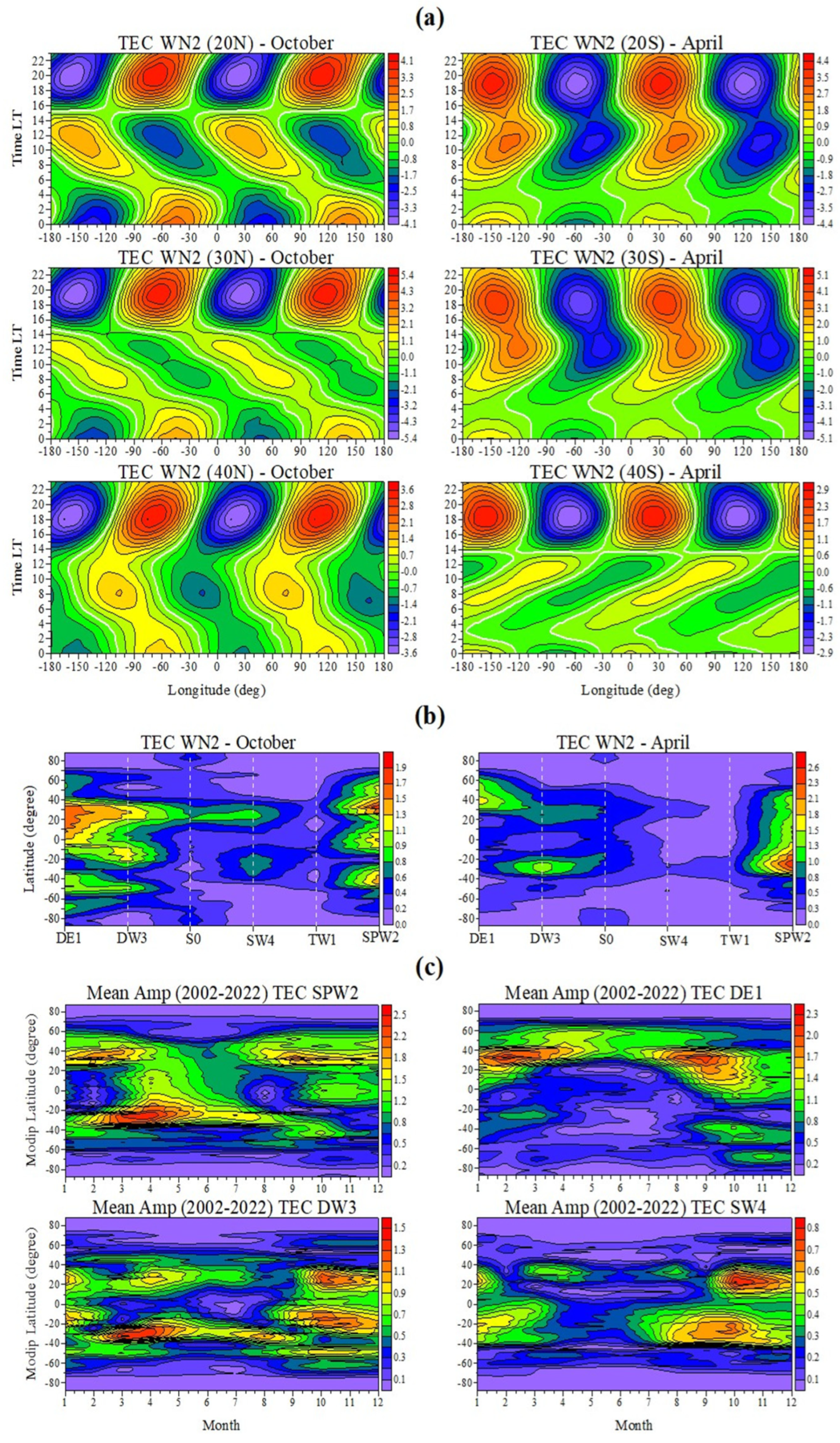
5.3. TEC WN2 Structure

The climatology of the TEC WN2 structure is calculated by the superposition of the same climatologically mean nonmigrating tides (and SPW2) as those in the lower thermosphere, i.e., DE1, DW3, S0, SW4, and TW1. Figure 14a shows the LT variability of the climatologically mean (2002–2022) TEC WN2 structure at different latitudes, shown in the upper side of each plot, during October for the NH and April for the SH. Similarly to the TEC WN3 structure, here, also, the seasonal dependence of the TEC WN2 structure is different from that of the SABER temperature WN2 one. The reason is again the prevailing ionospheric semiannual variability that has not been removed in advance. The main features of the climatologically mean TEC WN2 structure can be summarized as: (i) the immediately striking feature of this TEC structure in the latitude range ±40° is that it is significant mostly in the afternoon and evening hours, somewhere between 14–15 LT and 22–23 LT; (ii) in general, there is hemispheric asymmetry, as this time the NH structure is stronger than the SH one with an exception at ±20°; if we consider the strongest TEC WN2 at all latitudes, then this asymmetry is valid as well again without ±20°; (iii) this TEC structure reveals a second type of asymmetry in that the significant structures in the two hemispheres are out of phase in April and October; while the TEC WN2 maxima are centered at −150° and 30° in the SH, those in the NH are at −60° and 120°; (iv) besides the above-considered structures with the largest magnitude of 5.4 TECU, there are also weaker structures observed predominantly during early morning and daytime, between 04–05 LT and 14–15 LT; these TEC WN2 structures demonstrate the third type of asymmetry expressed in the reverse tilt of the structures; while they are tilted to the west in the NH, those of the SH are oriented to the east; (v) here, also, there are WN2 structures observed between 00 LT and 03–04 LT, but in general are not strong; however, at some latitudes, particularly in the NH, they are stronger than the daytime ones; and (vi) there is a feature, not shown in Figure 14a but which has to be mentioned, that at latitudes of ±50°, the strongest structures are the daytime ones seen between 06 LT and 18–19 LT, where again the NH WN2 magnitude (3.1 TECU) is larger than that of the SH (2.6 TECU).
In addition to October and April, large TEC WN2 magnitudes are also seen in March and November; the latter, however, are very similar to those in April and October. That is why Figure 14b presents the latitudinal dependence of the tidal and SPW2 contribution to the TEC WN2 structure only in October (left plot) and April (right plot). These results show that both the DE1 and SPW2 are the main contributors for the production of this structure, as the SPW2 is a larger than the DE1 contributor in April. The next contributor is DW3, followed by SW4, S0, and finally TW1. Figure 14c demonstrates the latitude-time climatological structures of the first four contributors to the TEC WN2 structures; these are the SPW2 (upper left plot), the DE1 (upper right plot), the DW3 (bottom left plot), and the SW4 (bottom right plot). The both factors connected with the hemispheric asymmetry of these components and their contributions to producing the TEC WN2 structure (Figure 14b) define the above-mentioned asymmetric features of this structure. Figure 14b,c also demonstrate why the TEC WN2 structure does not have small magnitudes at latitudes of ±50° (as 3.1 TECU) in comparison with those of WN4 and WN3 ones (as 0.9 TECU and 1.35 TECU, respectively).
Unfortunately, there is a paucity of information on the nonmigrating tides discussed above, and to what degree they are capable to penetrating into higher regions of the IT system. Forbes et al., 2014 [91], reported that the observed SW4 tide in the IT system is a combination of the in situ generated and propagating from below tide, while Jones et al., 2013 [95], obtained that the DE1 is in situ excited tide because the magnetic control of the ion-neutral interactions in the IT system.
In summary of Section 5, it should be noted that it examines in detail the climatological (2002–2022) features of the longitudinal TEC WN4, WN3, and WN2 structures in a way as they are present in the global TEC maps. The main reason is to quickly recognize these structures among the other ionospheric variations. However, this approach makes the longitudinal TEC structures dependent on the semiannual variability of the IT system, and to some extent this is a weak point of the present study. The only TEC structure that has not been affected by the semiannual IT variability is the WN4 one; most probably this is because the seasonal variability of the main contributor, the DE3, is similar to the IT semiannual one. It is worth noting that the above TEC longitudinal structures were successfully predicted for the first time by the empirical global TEC model.
The TEC WN3 structure is the strongest one with a maximum magnitude of 5.9 TECU. It shows a clear hemispheric asymmetry as the SH structure is stronger than the NH one, but only at latitudes of ±(30–50°). The main contributors to this TEC structure are the TEC SPW3 followed by TEC DE2. The second strongest TEC structure is the WN2 one with a maximum magnitude of 5.4 TECU. Generally, this structure also reveals a hemispheric asymmetry, but in this case, the NH structure is stronger than the SH one, with an exception at ±20°. The TEC SPW2 and TEC DE1 contribute the most for the production this structure. The weakest TEC structure is the WN4 one that has the largest amplitude of 3.7 TECU. It displays a clear hemispheric asymmetry, as the SH structure is stronger than the NH one at all latitudes. The TEC DE3 followed by the TEC SPW4 are the main contributors for this TEC structure. It is important to underline that all these magnitude maxima are located at the latitude of the EIA that is ±30° modip latitude.

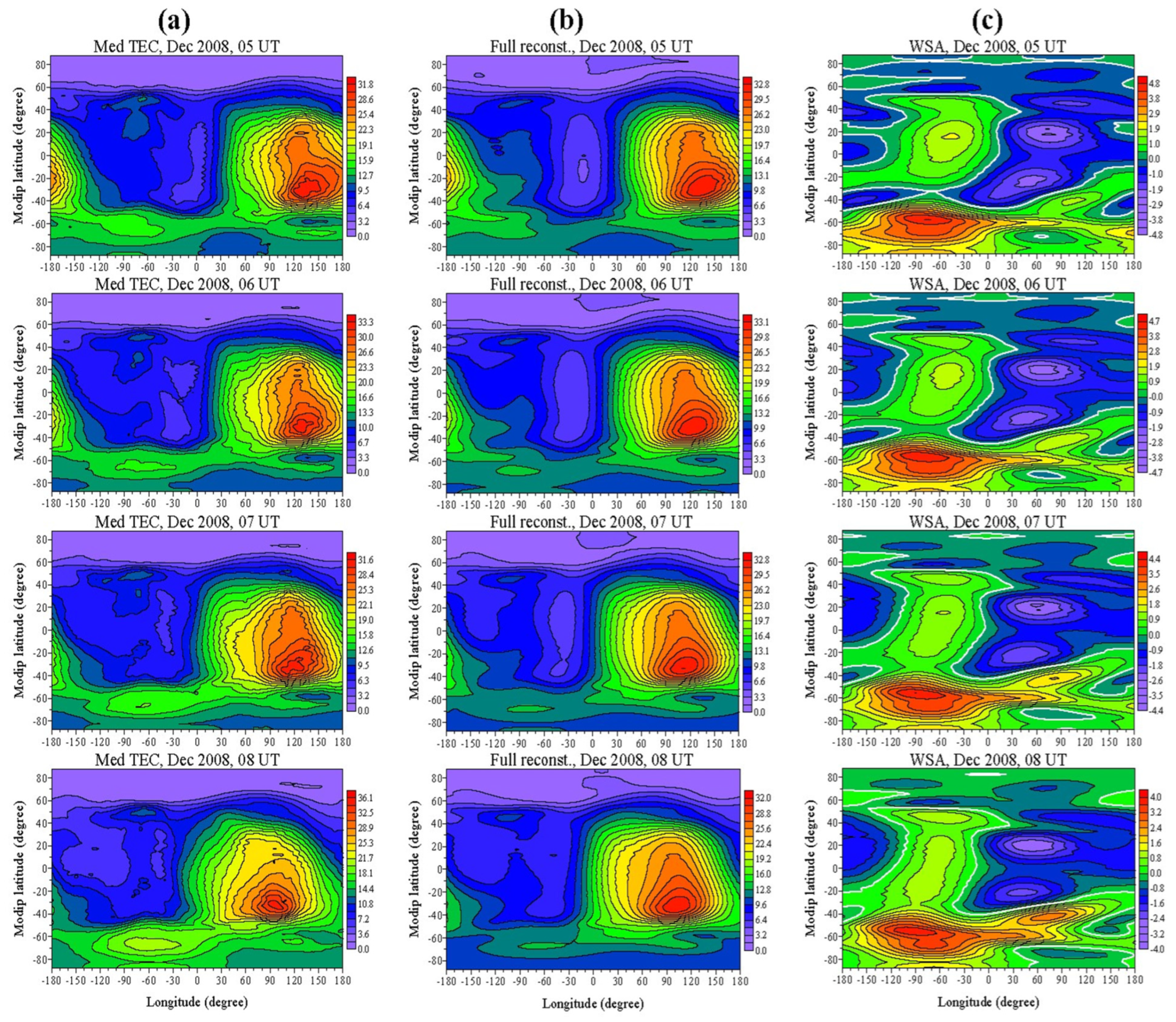
6. Weddell Sea Anomaly

The Weddell Sea Anomaly (WSA) appears in the region near the Weddell Sea and Antarctica peninsula and it characterized by the fact that the electron densities recurrently maximize during the local night-time in the austral summer [96]. This event was first detected in ionosonde measurements by Bellchambers and Piggott, 1958 [97]. However, the satellite observations of the WSA allowed its global structure to be examined more deeply [98,99]. The major physical mechanisms that have been suggested for the WSA formation are an equatorward neutral wind, an electric field, the photoionization, and the downward diffusion from the plasmasphere. A widely accepted explanation for the mechanism generating the WSA was reported by Dudeney and Piggott, 1978 [96], who attributed the WSA to a combination of thermosphere neutral winds and magnetic declination effects in the region of the Weddell Sea. The authors suggested that the summer neutral wind, directed from the higher latitudes to the equator, acts to transport plasma equatorward and upward along the magnetic field lines, where the plasma persists for a longer period of time, due to the reduced loss rate at higher altitudes. The magnetic dip angle around the Weddell Sea region is closer to 45°, and this allows the largest effective wind to be observed there. This leads to the largest amount of plasma drift along the field lines, causing an enhancement in the ionization at this longitudinal zone from plasma transported upward and equatorward from the summer high latitudes. Similar results were obtained by Hu et al., 2009 [100], based on more than two years of F3/C electron density profiles at low solar activities.
It has been mentioned before that, although traditionally applied mainly to the dynamics of the neutral middle atmosphere, the recent years have seen a growth in interest of applying the atmospheric tidal analysis to thermospheric and ionospheric parameters suggested for the first time by Pancheva and Mukhtarov, 2010 [26]. In the context of tides in the ionosphere and thermosphere Chen et al., 2013 [101], used the SAMI3 model coupled to the TIEGCM neutral winds to reproduce a realistic WSA, including the feature of eastward drift in a constant local time frame that was found in previous observations. Using Fourier analysis, it was found that the salient spatial and temporal features of the simulated WSA, including the eastward zonal drift and nighttime enhancement in the Weddell Sea region, could be attributed to a zonally symmetric diurnal tide, D0, responsible for 35% of the peak electron density anomaly at 300 km. The authors noted that the D0 component was also present in the vertical neutral winds along magnetic field lines in the southern mid to high latitude of the empirical Horizontal Wind Model 93, with phase structure suggesting in situ thermosphere generation. For the first time, however, the WSA has been successfully predicted by the global empirical TEC model established by Mukhtarov et al., 2013 [102], thanks to the nonmigrating tides and SPWs involved in it. The basic aim of this sub-section is to establish whether this long-known anomaly, which has so far been studied mostly on time-limited observations, can be observed in this case on a large statistics, and if so, what is its climatology. Only December and January will be considered because these are the months when the WSA most often manifests itself.
The first step is to define the main tidal and SPW components which contribute to the WSA production. Having in mind the main features of the WSA, briefly described above, such components among the tides could be only some diurnal tides with amplifications during austral summer and with phases maximizing around local midnight at mid-high southern latitudes; among the SWPs, this apparently could be only the SPW1. Knowing the main climatological (2002–2022) features of the TEC nonmigrating tides investigated in the present study such tides could be: (i) the zonally symmetric D0, because its recurrent enhancements in the austral summer around latitudes of ~60° S (Mukhtarov et al., 2013 [102]); (ii) the DW2 tide that reveals some enhancements in December-January at latitudes of ~40° S; and (iii) the DE1 having some secondary amplification in December–February at latitudes of ~65–70° S. All the above-mentioned nonmigrating tides are with phases maximizing around the local midnight. The SPW1 has a component that also amplifies at latitudes of ~60° S in December. Our result fully supports the previous WSA study reported by Chang et al., 2015 [103].
It is noted above that we are interested in the climatology of the WSA. This means that it is advisable to know in advance the nature of these nonmigrating tides, i.e., whether they are locally generated in the IT system, or are vertically upward-propagating from the lower atmosphere. It has been found before that the locally excited tides are strong during solar maximum (Jones et al., 2013 [95]) while the upward-propagating nonmigrating tides from the lower atmosphere are dominant at solar minimum [104]. If the above-mentioned nonmigrating tides belong to only one of type, then the WSA climatology probably could be under question. To clarify the nature of the considered nonmigrating tides, the F3/C electron density profiles for 2008 are analyzed in the same way as the SABER temperature and TEC data sets. We obtained, for December 2008, the same results as those of Chang et al., 2015 [103], with an exception related to the DW2 tide; we also obtained similar results for December 2011. Figure 15a shows the altitude-latitude structure of the DW2 amplitude (upper plot, in MHz) and phase (bottom plot, in degree) extracted from the FORMOSAT-3/COSMIC electron density profiles. There are two tidal amplifications, and of interest to us (i.e., it may contribute to the WSA production) is that situated around latitudes of (40–50°) S and altitudes of ~180–400 km; its phase structure clearly indicates a vertical upward propagation from below. Figure 15b demonstrates the latitude-time climatological (2002–2022) structure of the TEC DW2 tidal amplitude. In addition to the semiannual variability connected to changes in neutral thermospheric composition, it can be seen also in the DW2 enhancements in December around latitudes of −40° and 20–30°, which fully reflects the two amplifications seen in the upper plot of Figure 15a. It is worth noting that Figure 15a,b are obtained from two different data sets, and while Figure 15a presents a concrete observation, Figure 15b is a climatological result based on large statistics.
We, however, underline that the result of Figure 15a, indicating that the DW2 seen in the IT system, is vertically upward-propagating from below tide, contradicts not only to that of Chang et al., 2015 [103], but also to previous results based on simulations using the NCAR TIME-GSM [96] or a combination of satellite observations and employing Hough mode extensions (HMEs) and the Climatological Model of Thermosphere Tides (CTMT) [91]. This problem deserves to be more seriously investigated by simultaneous satellite observations of the MLT and IT system (especially the electron density measurements) based on larger statistics.
The next step is to make an attempt to reconstruct not only the WSA itself for different local times, but also the global distribution of TEC for December, first presenting the concrete results for December 2008 and then the corresponding climatological ones. Figure 16a displays the latitude-longitude structures of the median TEC for December 2008 at universal times: 05 UT (uppermost plot), 06 UT (second from above plot), 07 UT (second from below plot), and 08 UT (bottom plot) while Figure 16b presents the respective reconstructed TEC plots arranged in the same way as in Figure 16a. The careful inspection reveals very high degree of similarity between the observed and the reconstructed global TEC at the considered UTs; actually, these are nighttime local times at longitudes where the WSA is observed. Furthermore, the quality of the reconstruction is assessed by the RMSE which are for the considered universal times from 05 to 08 UT, respectively 1.174; 1.161; 1.151 and 1.133. These really very small errors unambiguously confirm the excellent reconstruction where the investigated WSA clearly stands out. Figure 16c demonstrates the latitude-longitude structure of the WSA itself reconstructed by the superposition of D0 + SPW1 + DW2 + DE1 at the above-mentioned UTs, arranged in the same way as in Figure 16a; actually, the real WSA is situated at the western part of the southern middle and high latitudes. These plots reveal that on the average the WSA is centered at longitude around 90°W and latitude of 60° S. Based on this, Figure 17a shows the latitude-time structures of the nonmigrating tidal D0 (left plot) DW2 (middle plot) and DE1 (right plot) amplitude at latitude of 60° S and longitude of 90°W for December 2008. It is seen that these tides have large effect mainly between 3–4 UT and 8–9 UT (i.e., between 21–22 and 2–3 LT), as well as at the range of the WSA, where the largest amplitude has the D0 followed by DW2 and finally is DE1. Figure 17b displays the latitudinal dependence of the tidal and SPW1 contribution to the WSA production in December 2008 at the following universal times: 05 UT (left plot), 06 UT (second from the left plot), 07 UT (second from the right plot), and 08 UT (right plot). Certainly the D0 has the largest contribution to the production of the WSA followed by the SPW1, DW2; then, finally, is DE1. Furthermore, there is also a decrease in the contribution of D0 and a concomitant increase in the contribution of SPW1 and DW2 with increasing UTs.
The last step in the analysis of the WSA is to check whether it is observed in our case in large statistics; this means we had to obtain the climatology of the distribution of the mean global TEC in December and January, which would show whether this anomaly is observed or not. While the results for December were definitely positive, in those for January, the WSA was hardly visible. Figure 18a produces the latitude-longitude structure of the climatological mean (2002–2022) TEC (left column of plots) and its full reconstruction (right column of plots) at universal times: 05 UT (uppermost plots), 06 UT (second from above plots), 07 UT (second from below plots), and 08 UT (bottom plots). Again, besides the high degree of similarity between both columns of plots, the reconstruction is assessed using the RMSE, which for the considered universal times from 05 to 08 UT are: 1.671, 1.607, 1.483, and 1.447, respectively. The results of Figure 18a clearly demonstrates the presence of the WSA in the climatologically (2002–2022) mean TEC in December, as well as the excellent reconstruction of this mean TEC assessed using the RMSE. Figure 18b shows the latitude-longitude structures of the climatological mean WSA itself (left column of plots), reconstructed by the superposition of the climatologically mean D0 + SPW1 + DW2 + DE1 and the latitudinal dependence of the contribution of these WSA components (right column of plots) at the above-mentioned UTs, arranged in the same way as in Figure 18a. In this case, the contribution of the DE1 is insignificant, while the contribution of the other components is the similar to that in December 2008.
Summarizing the results of Section 6 related to the WSA, we underline that the concrete analysis of December 2008 clearly revealed that not all tidal components contributing to the production of the WSA are in situ generated; the DW2, observed in the F3/C electron density profiles, is a tide propagating from below. The main result of this section, however, is the production of the global climatologically mean TEC only for December, where the WSA is very clearly visible as well as very well reconstructioned.

7. Summary

This paper presents the climatological features of the longitudinal structures WN4, WN3, and WN2 observed both in the lower thermospheric temperatures and in the ionospheric TEC observations. For this purpose, two long-term data sets are utilized: the satellite SABER/TIMED temperature measurements, and the global TEC maps generated with the NASA JPL Ionosphere Center for the interval of 2002–2022. The large statistics used in this study, based on 21 full years of observations, allows us to determine the spatial distribution and seasonal variability of the above-mentioned longitude structures with a high degree of probability.
The investigated WN4, WN3, and WN2 structures are produced by nonmigrating tides and zonally propagating planetary waves. Therefore, this study first investigates the climatological features of those nonmigrating tides, which are the main drivers of the above-mentioned longitude structures; these are the nonmigrating diurnal DE3, DE2, and DW2, and the semidiurnal SW4 and SE2 tides. The climatology of their spatial distribution, as well as the seasonal and interannual variability of the mentioned tides, are investigated in Section 3. Their climatological latitude and altitude-latitude structures, presented in Figure 1 and Figure 5, revealed that all these tides are vertically upward propagating and reach the largest amplitudes at or slightly above 110 km height. The main seasonal components for all nonmigrating tides under consideration turned out to be their annual means and annual and semiannual components. Their latitude-time structures, displayed in Figure 3 and Figure 7, demonstrate well evident interannual variations. Particular attention is paid to the stratospheric QBO index at 30 hPa; its impact on the seasonal components is studied using a cross correlation analysis. The seasonal components of the considered diurnal and semidiurnal nonmigrating tides in the lower thermosphere exhibit significant QBO variability, particularly the diurnal DE3 and DE2 tides (Figure 4 and Figure 8). The impact of the solar cycle has been investigated as well, but, in general, its effect on the considered nonmigrating tides is weak.
The climatological (2002–2022) features of the longitudinal WN4, WN3, and WN2 structures in the lower thermosphere (altitude of 110 km) are studied in detail in Section 4. The result for the WN4 (Figure 9) supports the previous ones, obtained on far smaller statistics, being that this is the strongest longitudinal structure in the lower thermosphere. We find that its largest climatological magnitude is ~20 K observed at 10° S in August. Additionally, the WN4 has larger magnitude in the SH than that in the NH, but only at latitudinal range of ±30°. The WN2 (Figure 11) is the second strongest structure, with magnitude reaching up to ~13.9 K at latitudes of 10° S in February; this structure demonstrates clear hemispheric asymmetry, as the SH structure is stronger than the NH one at the entire latitude range (±50°). The WN3 (Figure 10) is the weakest structure, with the largest magnitude of 12.4 K observed over the equator in July; this structure did not reveal clear hemispheric asymmetry. Besides the hemispheric asymmetry, latitude-seasonal, and some LT dependences, the above results are also supplemented with the assessment the latitudinal dependence of the contribution of each wave component in the production of the considered longitude structure.
The climatological features of the respective ionospheric longitudinal structures, presented in such a way as they are present in the global TEC maps, are examined in Section 5. The main reason for such approach is that these structures are able to be quickly recognized among the other ionospheric variations. The climatology of the ionospheric structures clearly indicates that the TEC WN3 (Figure 13) is the strongest one, with a maximum magnitude of 5.9 TECU located on the Southern crest of the EIA (at −30° modip latitude); it also shows a hemispheric asymmetry, as the SH structure is stronger than the NH one, but only at latitudes of ±(30–50°). The main contributors to this TEC structure turns out to be first the TEC SPW3 followed by the TEC DE2. The second strongest TEC structure is the WN2 one (Figure 14), with the largest magnitude of 5.4 TECU seen on the Northern ridge of the EIA (at 30° modip latitude). Generally, this structure also reveals a hemispheric asymmetry, but in this case, the NH structure is stronger than the SH one, with an exception at ±20°. In this case, the TEC SPW2 is the strongest contributor, followed by the TEC DE1. The weakest TEC structure is the WN4 one (Figure 12) that has the largest amplitude of 3.7 TECU observed on the Southern crest of the EIA. It displays a clear hemispheric asymmetry at all latitudes, as the SH structure is stronger than the NH one. In general, the TEC DE3 is the main contributor, while the TEC SPW4 is the second one, to the production of the TEC WN4 structure.
The last result of this paper is presented in Section 6, and it is related to the well-known Weddell Sea Anomaly. Its detailed investigation revealed that not all wave components leading to the WSA production are in situ generated; the non-migrating DW2 tide is a propagating from below tide. This study demonstrates, for the first time, the climatology of the WSA based on the full 21 years, as well as its very good reconstruction (Figure 18). This result is also supplemented by the assessment of the contribution of each climatologically mean wave component in building up this anomaly.
In conclusion, we note that, by means of a detailed analysis with the same method of two long-term data sets representing the wave forcing from the MLT region and the respective ionospheric TEC response, we present valuable climatological evidence for recognizing regular TEC structures generated by lower atmospheric weather systems. It is worth noting that the longitudinal TEC structures considered in this paper are weaker than geomagnetic anomalies, but, in contrast, they are almost constantly present in the ionosphere and have well-defined seasonal and latitudinal dependences; the latter make them predictable. Additionally, the MLT tidal diagnostics, based on the large statistics presented in this overview paper, provides the necessary observational constraints for the numerical simulations.

Author Contributions

Conceptualization, D.P. and P.M.; methodology, D.P.; software, P.M.; validation, D.P. and P.M.; formal analysis, D.P.; investigation, D.P.; resources, P.M.; writing—original draft preparation, D.P.; writing—review and editing, D.P. and R.B.; visualization, D.P., P.M. and R.B.; supervision, D.P. All authors have read and agreed to the published version of the manuscript.

Funding

This work was supported by the National Science Fund under Competition for financial support of basic research projects—2020, grant No KP-06-H44/2 from 27 November 2020 “Space weather over a period of the century solar activity descending”.

Institutional Review Board Statement

Not applicable.

Informed Consent Statement

Not applicable.

Data Availability Statement

The SABER temperature data version 2.0, level 2A, are downloaded from: https://saber.gats-inc.com/data.php (accessed on 10 April 2024). The vertical TEC maps generated with the NASA JPL (Jet Propulsion Laboratory, California Institute of Technology, USA) IGS Ionosphere Center are provided by: https://sideshow.jpl.nasa.gov/pub/iono_daily/IONEX_rapid (accessed on 10 April 2024). However, the TEC data analyzed were downloaded from: https://www.izmiran.ru/ionosphere/weather/grif/Maps/TEC/ (accessed on 9 April 2024). The solar radio flux index F10.7 data were downloaded from the website: https://omniweb.gsfc.nasa.gov/ow.html (accessed on 10 April 2024). The QBO index at 30 hPa is obtained from https://www.cpc.ncep.noaa.gov/data/indices/ (accessed on 10 April 2024). We note that the electron density data were downloaded quite long time ago from the website. Unfortunately, the above-mentioned website is no longer active.

Acknowledgments

The authors express their gratitude to all above-mentioned Scientific Data Centers which kindly provided all data used in this study. They would also like to thank both anonymous reviewers for their generally positive opinion about our results and insightful comments, which helped to improve the overall quality of the paper.

Conflicts of Interest

The authors declare no conflicts of interest.

References

  1. Chapman, S.; Lindzen, R.S. Atmospheric Tides: Thermal and Gravitational, 1st ed.; Springer: Dordrecht, The Netherlands, 1970; pp. 1–200. [Google Scholar] [CrossRef]
  2. Kato, S. Non-migrating tides. J. Atmos. Terr. Phys. 1989, 51, 673–682. [Google Scholar] [CrossRef]
  3. Hagan, M.E.; Roble, R.G. Modeling diurnal tidal variability with the National Center for Atmospheric Research thermosphere-ionosphere-mesosphere-electrodynamics general circulation model. J. Geophys. Res. Space Phys. 2001, 106, 24869–24882. [Google Scholar] [CrossRef]
  4. Angelats, I.; Coll, M.; Forbes, J.M. Nonlinear interactions in the upper atmosphere: The s = 1 and s = 3 nonmigrating semidiurnal tides. J. Geophys. Res. Space Phys. 2002, 107, 1157–1171. [Google Scholar] [CrossRef]
  5. Forbes, J.M.; Wu, D. Solar tides as revealed by measurements of mesosphere temperature by the MLS experiment on UARS. J. Atmos. Sci. 2006, 63, 1776–1797. [Google Scholar] [CrossRef]
  6. Pancheva, D.; Mukhtarov, P.; Andonov, B. Nonmigrating tidal activity related to the sudden stratospheric warming in the Arctic winter of 2003/2004. Ann. Geophys. 2009, 27, 975–987. [Google Scholar] [CrossRef]
  7. Hamilton, K. Latent heat release as a possible forcing mechanism for atmospheric tides. Mon. Weather Rev. 1981, 109, 3–17. [Google Scholar] [CrossRef]
  8. Hagan, M.E.; Forbes, J.M. Migrating and nonmigrating diurnal tides in the middle and upper atmosphere excited by tropical latent heat release. J. Geophys. Res. Atmos. 2002, 107, 4754–4768. [Google Scholar] [CrossRef]
  9. Oberheide, J.; Hagan, M.E.; Roble, R.G.; Offermann, D. Sources of nonmigrating tides in the tropical middle atmosphere. J. Geophys. Res. Atmos. 2002, 107, 4567–4580. [Google Scholar] [CrossRef]
  10. Zhang, X.; Forbes, J.M.; Hagan, M.E. Longitudinal variation of tides in the MLT region: 2. Relative effects of solar radiative and latent heating. J. Geophys. Res. Space Phys. 2010, 115, 1–19. [Google Scholar] [CrossRef]
  11. Miyoshi, Y.; Pancheva, D.; Mukhtarov, P.; Jin, H.; Fujiwara, H.; Shinagawa, H. Excitation mechanism of non-migrating tides. J. Atmos. Sol.-Terr. Phys. 2017, 156, 24–36. [Google Scholar] [CrossRef]
  12. Hagan, M.E.; Forbes, J.M. Migrating and nonmigrating semidiurnal tides in the upper atmosphere excited by tropospheric latent heat release. J. Geophys. Res. Space Phys. 2003, 108, 1062–1075. [Google Scholar] [CrossRef]
  13. Lieberman, R.S. Nonmigrating diurnal tides in the equatorial middle atmosphere. J. Atmos. Sci. 1991, 48, 1112–1123. [Google Scholar] [CrossRef]
  14. Talaat, E.R.; Lieberman, R.S. Nonmigrating diurnal tides in mesospheric and lower thermospheric winds and temperatures. J. Atmos. Sci. 1999, 56, 4073–4087. [Google Scholar] [CrossRef]
  15. Oberheide, J.; Gusev, O.A. Observations of migrating and nonmigrating diurnal tides in the equatorial lower thermosphere. Geophys. Res. Lett. 2002, 29, 2167–2170. [Google Scholar] [CrossRef]
  16. Forbes, J.M.; Zhang, X.; Talaat, E.R.; Ward, W. Nonmigrating diurnal tides in the thermosphere. J. Geophys. Res. Space Phys. 2003, 108, 1033–1042. [Google Scholar] [CrossRef]
  17. Forbes, J.M.; Russell, J.; Miyahara, S.; Zhang, X.; Palo, S.; Mlynczak, M.; Mertens, C.J.; Hagan, M.E. Troposphere–thermosphere tidal coupling as measured by the SABER instrument on TIMED during July–September 2002. J. Geophys. Res. Space Phys. 2006, 111, 1–15. [Google Scholar] [CrossRef]
  18. Huang, F.T.; Reber, C.A. Nonmigrating semidiurnal and diurnal tides at 95 km based on wind measurements from the High Resolution Doppler Imager on UARS. J. Geophys. Res. Atmos. 2004, 109, 1–13. [Google Scholar] [CrossRef]
  19. Lieberman, R.; Oberheide, J.; Hagan, M.; Remsberg, E.; Gordley, L. Variability of diurnal tides and planetary waves during November 1978–May 1979. J. Atmos. Sol.-Terr. Phys. 2004, 66, 517–528. [Google Scholar] [CrossRef]
  20. Mukhtarov, P.; Pancheva, D.; Andonov, B. Global structure and seasonal and interannual variability of the migrating diurnal tide seen in the SABER/TIMED temperatures between 20 and 120 km. J. Geophys. Res. Space Phys. 2009, 114, 1–17. [Google Scholar] [CrossRef]
  21. Pancheva, D.; Mukhtarov, P. Atmospheric tides and planetary waves: Recent progress based on SABER/TIMED temperature measurements (2002–2007). In Aeronomy of the Earth’s Atmosphere and Ionosphere, 1st ed.; IAGA Special Sopron Book Series; Abdu, M., Pancheva, D., Eds.; Springer: Dordrecht, The Netherlands, 2011; Volume 2, pp. 19–56. [Google Scholar] [CrossRef]
  22. Zhang, X.; Forbes, J.M.; Hagan, M.E.; Russell, J.M., III; Palo, S.E.; Mertens, C.J.; Mlynczak, M.G. Monthly tidal temperatures 20–120 km from TIMED/SABER. J. Geophys. Res. Space Phys. 2006, 111, 1–20. [Google Scholar] [CrossRef]
  23. Forbes, J.M.; Zhang, X.; Palo, S.; Russell, J.; Mertens, C.J.; Mlynczak, M. Tidal variability in the ionospheric dynamo region. J. Geophys. Res. Space Phys. 2008, 113, 1–17. [Google Scholar] [CrossRef]
  24. Oberheide, J.; Wu, Q.; Killeen, T.L.; Hagan, M.E.; Roble, R.G. Diurnal nonmigrating tides from TIMED Doppler Interferometer wind data: Monthly climatologies and seasonal variations. J. Geophys. Res. Space Phys. 2006, 111, 1–22. [Google Scholar] [CrossRef]
  25. Oberheide, J.; Wu, Q.; Killeen, T.L.; Hagan, M.E.; Roble, R.G. A climatology of nonmigrating semidiurnal tides from TIMED Doppler Interferometer (TIDI) wind data. J. Atmos. Sol.-Terr. Phys. 2007, 69, 2203–2218. [Google Scholar] [CrossRef]
  26. Pancheva, D.; Mukhtarov, P. Strong evidence for the tidal control on the longitudinal structure of the ionospheric F-region. Geophys. Res. Lett. 2010, 37, 1–5. [Google Scholar] [CrossRef]
  27. Pancheva, D.; Mukhtarov, P.; Andonov, B. Global structure, seasonal and interannual variability of the eastward propagating tides seen in the SABER/TIMED temperatures (2002–2007). Adv. Space Res. 2010, 46, 257–274. [Google Scholar] [CrossRef]
  28. Oberheide, J.; Forbes, J.M.; Zhang, X.; Bruinsma, S.L. Wave-driven variability in the ionosphere-thermosphere-mesosphere system from TIMED observations: What contributes to the “wave 4”? J. Geophys. Res. Space Phys. 2011, 116, 1–15. [Google Scholar] [CrossRef]
  29. Wan, W.; Xu, J. Recent investigation on the coupling between the ionosphere and upper atmosphere. Sci. China Earth Sci. 2014, 57, 1995–2012. [Google Scholar] [CrossRef]
  30. Li, X.; Wan, W.; Ren, Z.; Liu, L.; Ning, B. The variability of nonmigrating tides detected from TIMED/SABER observations. J. Geophys. Res. Space Phys. 2015, 120, 10793–10808. [Google Scholar] [CrossRef]
  31. Pancheva, D.; Mukhtarov, P.; Smith, A.K. Nonmigrating tidal variability in the SABER/TIMED mesospheric ozone. Geophys. Res. Lett. 2014, 41, 4059–4067. [Google Scholar] [CrossRef]
  32. Li, X.; Wan, W.; Ren, Z.; Yu, Y. The variability of SE2 tide extracted from TIMED/SABER observations. J. Geophys. Res. Space Phys. 2017, 122, 2136–2150. [Google Scholar] [CrossRef]
  33. Li, X.; Ren, Z.; Cao, J. The Spatiotemporal Variability of Non-Migrating Tides in the Zonal Wind Component Detected From TIMED/TIDI Observations. J. Geophys. Res. Space Phys. 2023, 128, e2022JA030879. [Google Scholar] [CrossRef]
  34. Sagawa, E.; Immel, T.J.; Frey, H.U.; Mende, S.B. Longitudinal structure of the equatorial anomaly in the nighttime ionosphere observed by IMAGE/FUV. J. Geophys. Res. Space Phys. 2005, 110, 1–10. [Google Scholar] [CrossRef]
  35. Immel, T.J.; Sagawa, E.; England, S.L.; Henderson, S.B.; Hagan, M.E.; Mende, S.B.; Frey, H.U.; Swenson, C.M.; Paxton, L.J. Control of equatorial ionospheric morphology by atmospheric tides. Geophys. Res. Lett. 2006, 33, 1–4. [Google Scholar] [CrossRef]
  36. Kil, H.; Oh, S.J.; Kelley, M.C.; Paxton, L.J.; England, S.L.; Talaat, E.; Min, K.W.; Su, S.Y. Longitudinal structure of the vertical E× B drift and ion density seen from ROCSAT-1. Geophys. Res. Lett. 2007, 34, 1–5. [Google Scholar] [CrossRef]
  37. Kil, H.; Talaat, E.R.; Oh, S.J.; Paxton, L.J.; England, S.L.; Su, S.Y. The wave structures of the plasma density and vertical E × B drift in low-latitude F region. J. Geophys. Res. Space Phys. 2008, 113, 1–12. [Google Scholar] [CrossRef]
  38. Richmond, A.D. The ionospheric wind dynamo: Effects of its coupling with different atmospheric regions. In The Upper Mesosphere and Lower Thermosphere: A Review of Experiments and Theory; As Part of the Geophysical Monograph Series; Johnson, R.M., Killeen, T.L., Eds.; American Geophysical Union (AGU): Washington, DC, USA, 1995; Volume 87, pp. 49–65. [Google Scholar] [CrossRef]
  39. Heelis, R.A. Electrodynamics in the low and middle latitude ionosphere: A tutorial. J. Atmos. Sol.-Terr. Phys. 2004, 66, 825–838. [Google Scholar] [CrossRef]
  40. England, S.L.; Immel, T.J.; Huba, J.D.; Hagan, M.E.; Maute, A.; DeMajistre, R. Modeling of multiple effects of atmospheric tides on the ionosphere: An examination of possible coupling mechanisms responsible for the longitudinal structure of the equatorial ionosphere. J. Geophys. Res. Space Phys. 2010, 115, 1–13. [Google Scholar] [CrossRef]
  41. England, S.L. Review of the effects of non-migrating atmospheric tides on Earth’s low-latitude ionosphere. Space Sci. Rev. 2012, 168, 211–236. [Google Scholar] [CrossRef]
  42. England, S.L.; Immel, T.J.; Sagawa, E.; Henderson, S.B.; Hagan, M.E.; Mende, S.B.; Frey, H.U.; Swenson, C.M.; Paxton, L.J. Effect of atmospheric tides on the morphology of the quiet-time post-sunset equatorial ionospheric anomaly. J. Geophys. Res. Space Phys. 2006, 111, 1–12. [Google Scholar] [CrossRef]
  43. Hartman, W.A.; Heelis, R.A. Longitudinal variations in the equatorial vertical drift in the topside ionosphere. J. Geophys. Res. Space Phys. 2007, 112, 1–6. [Google Scholar] [CrossRef]
  44. Ren, Z.; Wan, W.; Liu, L.; Zhao, B.; Wei, Y.; Yue, X.; Heelis, R.A. Longitudinal variations of electron temperature and total ion density in the sunset equatorial topside ionosphere. Geophys. Res. Lett. 2008, 35, 1–4. [Google Scholar] [CrossRef]
  45. England, S.L.; Maus, S.; Immel, T.J.; Mende, S.B. Longitudinal variation of the E-region electric fields caused by atmospheric tides. Geophys. Res. Lett. 2006, 33, 1–5. [Google Scholar] [CrossRef]
  46. Lühr, H.; Rother, M.; Häusler, K.; Alken, P.; Maus, S. Influence of nonmigrating tides on the longitudinal variations of the equatorial electrojet. J. Geophys. Res. Space Phys. 2008, 113, 1–8. [Google Scholar] [CrossRef]
  47. Häusler, K.; Lühr, H.; Rentz, S.; Köhler, W. A statistical analysis of longitudinal dependences of upper thermospheric zonal winds at dip equator latitudes derived from CHAMP. J. Atmos. Sol.-Terr. Phys. 2007, 69, 1419–1430. [Google Scholar] [CrossRef]
  48. Zhang, K.; Wang, W.; Wang, H.; Dang, T.; Liu, J.; Wu, Q. The longitudinal variations of upper thermospheric zonal winds observed by the CHAMP satellite at low and midlatitudes. J. Geophys Res. Space Phys. 2018, 123, 9652–9668. [Google Scholar] [CrossRef]
  49. Lin, C.H.; Hsiao, C.C.; Liu, J.Y.; Liu, C.H. Longitudinal structure of the equatorial ionosphere: Time evolution of the four-peaked EIA structure. J. Geophys. Res. Space Phys. 2007, 112, 1–8. [Google Scholar] [CrossRef]
  50. Häusler, K.; Lühr, H. Nonmigrating tidal signals in the upper thermospheric zonal wind at equatorial latitudes as observed by CHAMP. Ann. Geophys. 2009, 27, 2643–2652. [Google Scholar] [CrossRef]
  51. Wan, W.; Liu, L.; Pi, X.; Zhang, M.L.; Ning, B.; Xiong, J.; Ding, F. Wavenumber-4 patterns of the total electron content over the low latitude ionosphere. Geophys. Res. Lett. 2008, 35, 1–5. [Google Scholar] [CrossRef]
  52. Fejer, B.G.; Jensen, J.W.; Su, S.Y. Quiet time equatorial F region vertical plasma drift model derived from ROCSAT-1 observations. J. Geophys. Res. Space Phys. 2008, 113, 1–10. [Google Scholar] [CrossRef]
  53. Bankov, L.; Heelis, R.; Parrot, M.; Berthelier, J.J.; Marinov, P.; Vassileva, A. WN4 effect on longitudinal distribution of different ion species in the topside ionosphere at low latitudes by means of DEMETER, DMSP-F13 and DMSP-F15 data. Ann. Geophys. 2009, 27, 2893–2902. [Google Scholar] [CrossRef]
  54. Liu, H.; Yamamoto, M.; Lühr, H. Wave-4 pattern of the equatorial mass density anomaly: A thermospheric signature of tropical deep convection. Geophys. Res. Lett. 2009, 36, 1–4. [Google Scholar] [CrossRef]
  55. Pancheva, D.; Mukhtarov, P. Global Response of the Ionosphere to Atmospheric Tides Forced from Below: Recent Progress Based on Satellite Measurements: Global Tidal Response of the Ionosphere. Space Sci. Rev. 2012, 168, 175–209. [Google Scholar] [CrossRef]
  56. Mukhtarov, P.; Pancheva, D. Global ionospheric response to nonmigrating DE3 and DE2 tides forced from below. J. Geophys. Res. Space Phys. 2011, 116, 1–16. [Google Scholar] [CrossRef]
  57. Pancheva, D.; Miyoshi, Y.; Mukhtarov, P.; Jin, H.; Shinagawa, H.; Fujiwara, H. Global response of the ionosphere to atmospheric tides forced from below: Comparison between COSMIC measurements and simulations by atmosphere ionosphere coupled model GAIA. J. Geophys. Res. Space Phys. 2012, 117, 1–19. [Google Scholar] [CrossRef]
  58. Miyoshi, Y.; Fujiwara, H. Day-to-day variations of migrating diurnal tide simulated by a GCM from the ground surface to the exobase. Geophys. Res. Lett. 2003, 30, 1789–1793. [Google Scholar] [CrossRef]
  59. Shinagawa, H. Ionosphere simulation. J. Natl. Inst. Comm. Technol. 2009, 56, 199–207. [Google Scholar]
  60. Jin, H.; Miyoshi, Y.; Fujiwara, H.; Shinagawa, H.; Terada, K.; Terada, N.; Ishii, M.; Otsuka, Y.; Saito, A. Vertical connection from the tropospheric activities to the ionospheric longitudinal structure simulated by a new Earth’s whole atmosphere-ionosphere coupled model. J. Geophys. Res. Space Phys. 2011, 116, 1–9. [Google Scholar] [CrossRef]
  61. Jin, H.; Miyoshi, Y.; Fujiwara, H.; Shinagawa, H. Electrodynamics of the formation of ionospheric wave number 4 longitudinal structure. J. Geophys. Res. Space Phys. 2008, 113, 1–7. [Google Scholar] [CrossRef]
  62. Ren, Z.; Wan, W.; Xiong, J.; Liu, L. Simulated wave number 4 structure in equatorial F-region vertical plasma drifts. J. Geophys. Res. Space Phys. 2010, 115, A05301. [Google Scholar] [CrossRef]
  63. England, S.L.; Zhang, X.; Immel, T.J.; Forbes, J.M.; DeMajistre, R. The effect of non-migrating tides on the morphology of the equatorial ionospheric anomaly: Seasonal variability. Earth Planets Space 2009, 61, 493–503. [Google Scholar] [CrossRef]
  64. Pedatella, N.M.; Forbes, J.M.; Oberheide, J. Intra-annual variability of the low-latitude ionosphere due to nonmigrating tides. Geophys. Res. Lett. 2008, 35, 1–4. [Google Scholar] [CrossRef]
  65. Mertens, C.J.; Mlynczak, M.; Lopez-Puertas, M.; Wintersteiner, P.P.; Picard, R.H.; Winick, J.R.; Gordley, L.L.; Russell III, J.M. Retrieval of mesospheric and lower thermospheric kinetic temperature from measurements of CO2 15μm earth limb emission under non-LTE conditions. Geophys. Res. Lett. 2001, 28, 1391–1394. [Google Scholar] [CrossRef]
  66. Mertens, C.J.; Schmidlin, F.J.; Goldberg, R.A.; Remsberg, E.E.; Pesnell, W.D.; Russell III, J.M.; Mlynczak, M.G.; Lopez-Puertas, M.; Wintersteiner, P.P.; Picard, R.H.; et al. SABER observations of mesospheric temperatures and comparisons with falling sphere measurements taken during the 2002 summer MaCWAVE campaign. Geophys. Res. Lett. 2004, 31, 1–5. [Google Scholar] [CrossRef]
  67. Christensen, A.B.; Bishop, R.L.; Budzien, S.A.; Hecht, J.H.; Mlynczak, M.G.; Russell III, J.M.; Stephan, A.W.; Walterscheid, R.W. Altitude profiles of lower thermospheric temperature from RAIDS/NIRS and TIMED/SABER remote sensing experiments. J. Geophys. Res. Space Phys. 2013, 118, 3740–3746. [Google Scholar] [CrossRef]
  68. Remsberg, E.E.; Marshall, B.T.; Garcia-Comas, M.; Krueger, D.; Lingenfelser, G.S.; Martin-Torres, J.; Mlynczak, M.G.; Russell III, J.M.; Smith, A.K.; Zhao, Y.; et al. Assessment of the quality of the Version 1.07 temperature-versus-pressure profiles of the middle atmosphere from TIMED/SABER. J. Geophys. Res. Atmos. 2008, 113, 1–27. [Google Scholar] [CrossRef]
  69. García-Comas, M.; López-Puertas, M.; Marshall, B.T.; Wintersteiner, P.P.; Funke, B.; Bermejo-Pantaleón, D.; Mertens, C.J.; Remsberg, E.E.; Gordley, L.L.; Mlynczak, M.G.; et al. Errors in Sounding of the Atmosphere using Broadband Emission Radiometry (SABER) kinetic temperature caused by non-local-thermodynamic-equilibrium model parameters. J. Geophys. Res. Atmos. 2008, 113, 1–16. [Google Scholar] [CrossRef]
  70. Dawkins, E.C.M.; Feofilov, A.; Rezac, L.; Kutepov, A.A.; Janches, D.; Höffner, J.; Chu, X.; Lu, X.; Mlynczak, M.G.; Russell, J., III. Validation of SABER v2.0 operational temperature data with ground-based lidars in the mesosphere-lower thermosphere region (75–105 km). J. Geophys. Res. Atmos. 2018, 123, 9916–9934. [Google Scholar] [CrossRef]
  71. Pancheva, D.; Mukhtarov, P. Climatology and interannual variability of the migrating quarterdiurnal tide (QW4) seen in the SABER/TIMED temperatures (2002–2022). J. Atmos. Sol.-Terr. Phys. 2023, 250, 106111. [Google Scholar] [CrossRef]
  72. Pancheva, D.; Mukhtarov, P.; Andonov, B. Global structure, seasonal and interannual variability of the migrating semidiurnal tide seen in the SABER/TIMED temperatures (2002–2007). Ann. Geophys. 2009, 27, 687–703. [Google Scholar] [CrossRef]
  73. Ho, C.M.; Mannucci, A.J.; Lindqwister, U.J.; Pi, X.; Tsurutani, B.T. Global ionosphere perturbations monitored by the orldwide GPS network. Geophys. Res. Lett. 1996, 23, 3219–3222. [Google Scholar] [CrossRef]
  74. Rawer, K. Meteorological and astronomical influences on radio wave propagation. In Proceedings of Papers Read at the NATO Advanced Study Institute; Corfu, 1961; Landmark, B., Ed.; Pergamon Press: Oxford, UK, 1963; Volume 3, pp. 221–250. [Google Scholar]
  75. Azpilicueta, F.; Brunini, C.; Radicella, S.M. Global ionospheric maps from GPS observations using modip latitude. Adv. Space Res. 2006, 38, 2324–2331. [Google Scholar] [CrossRef]
  76. Lei, J.; Syndergaard, S.; Burns, A.G.; Solomon, S.C.; Wang, W.; Zeng, Z.; Roble, R.G.; Wu, Q.; Kuo, Y.H.; Holt, J.M.; et al. Comparison of COSMIC ionospheric measurements with ground-based observations and model predictions: Preliminary results. J. Geophys. Res. Space Phys. 2007, 112, 1–10. [Google Scholar] [CrossRef]
  77. Cheng, C.Z.; Kuo, Y.H.; Anthes, R.A.; Wu, L. Satellite constellation monitors global and space weather. EOS Trans. 2006, 87, 166. [Google Scholar] [CrossRef]
  78. Tokioka, T.; Yagai, I. Atmospehric tides appearing in a global atmospheric general circulation model. J. Meteorol. Soc. Jpn. Ser. II 1987, 65, 423–438. [Google Scholar] [CrossRef]
  79. Niu, X.; Du, J.; Zhu, X. Statistics on Nonmigrating Diurnal Tides Generated by Tide-Planetary Wave Interaction and Their Relationship to Sudden Stratospheric Warming. Atmosphere 2018, 9, 416. [Google Scholar] [CrossRef]
  80. Forbes, J.M.; Zhang, X.; Marsh, D.R. Solar cycle dependence of middle atmosphere temperatures. J. Geophys. Res. Atmos. 2014, 119, 9615–9625. [Google Scholar] [CrossRef]
  81. Nath, O.; Sridharan, S. Long-term variabilities and tendencies in zonal mean TIMED–SABER ozone and temperature in the middle atmosphere at 10–158 N. J. Atmos. Sol.-Terr. Phys. 2014, 120, 1–8. [Google Scholar] [CrossRef]
  82. Holton, J.R.; Tan, H.C. The influence of the equatorial quasi-biennial oscillation on the global circulation at 50 mb. J. Atmos. Sci. 1980, 37, 2200–2208. [Google Scholar] [CrossRef]
  83. Hagan, M.E.; Maute, A.I.; Roble, R.G. Tropospheric tidal effects on the middle and upper atmosphere. J. Geophys. Res. Space Phys. 2009, 114, 1–6. [Google Scholar] [CrossRef]
  84. Truskowski, A.O.; Forbes, J.M.; Zhang, X.; Palo, S.E. New perspectives on thermosphere tides: 1. Lower thermosphere spectra and seasonal-latitudinal structures. Earth Planets Space 2014, 66, 136. [Google Scholar] [CrossRef]
  85. Moudden, Y.; Forbes, J.M. A decade-long climatology of terdiurnal tides using TIMED/SABER observations. J. Geophys. Res. Space Phys. 2013, 118, 4534–4550. [Google Scholar] [CrossRef]
  86. Oberheide, J.; Forbes, J.M. Thermospheric nitric oxide variability induced by nonmigrating tides. Geophys. Res. Lett. 2008, 35, 1–5. [Google Scholar] [CrossRef]
  87. Barth, C.A.; Mankoff, K.D.; Bailey, S.M.; Solomon, S.C. Global observations of nitric oxide in the thermosphere. J. Geophys. Res. Space Phys. 2003, 108, 1–11. [Google Scholar] [CrossRef]
  88. Li, D.; Gao, H.; Xu, J.; Zhu, Y.; Xu, Q.; Liu, Y.; Liu, H. Longitudinal structures of zonal wind in the thermosphere by the ICON/MIGHTI and the main wave sources. Earth Planets Space 2023, 75, 59. [Google Scholar] [CrossRef]
  89. Chang, L.C.; Lin, C.H.; Liu, J.Y.; Balan, N.; Yue, J.; Lin, J.T. Seasonal and local time variation of ionospheric migrating tides in 2007–2011 FORMOSAT-3/COSMIC and TIE-GCM total electron content. J. Geophys. Res. Space Phys. 2013, 118, 2545–2564. [Google Scholar] [CrossRef]
  90. Wang, S.; Huang, S.; Fang, H. Wave-3 and wave-4 patterns in the low- and mid-latitude ionospheric TEC. J. Atmos. Sol.-Terr. Phys. 2015, 132, 82–91. [Google Scholar] [CrossRef]
  91. Forbes, J.M.; Zhang, X.; Bruinsma, S.L. New perspectives on thermospheric tides: 2. penetration to the upper thermosphere. Earth Planets Space 2014, 66, 122. [Google Scholar] [CrossRef]
  92. Hagan, M.E.; Maute, A.; Roble, R.G.; Richmond, A.D.; Immel, T.J.; England, S.L. Connections between deep tropical clouds and the Earth’s ionosphere. Geophys. Res. Lett. 2007, 34, 1–4. [Google Scholar] [CrossRef]
  93. Fuller-Rowell, T.J. The ‘thermospheric spoon’: A mechanism for the semi-annual density variation. J. Geophys. Res. Space Phys. 1998, 103, 3951–3956. [Google Scholar] [CrossRef]
  94. Qian, L.; Burns, A.G.; Solomon, S.C.; Wang, W. Annual/semiannual variation of the ionosphere. Geophys. Res. Lett. 2013, 40, 1928–1933. [Google Scholar] [CrossRef]
  95. Jones, M., Jr.; Forbes, J.M.; Hagan, M.E.; Maute, A. Non-migrating tides in the ionosphere-thermosphere: In situ versus tropospheric sources. J. Geophys. Res. Space Phys. 2013, 118, 2438–2451. [Google Scholar] [CrossRef]
  96. Dudeney, J.R.; Piggott, W.R. Antarctic ionospheric research. In Upper Atmosphere Research in Antarctica; Lanzerotti, L.J., Park, C.G., Eds.; AGU: Washington, DC, USA, 1978; Volume 29, pp. 200–235. 029p. [Google Scholar]
  97. Bellchambers, W.H.; Piggott, W.R. Ionospheric measurements made at Halley Bay. Nature 1958, 182, 1596–1597. [Google Scholar] [CrossRef]
  98. Horvath, I.; Essex, E.A. The Weddell Sea Anomaly observed with the Topex satellite data. J. Atmos. Sol. Terr. Phys. 2003, 65, 693–706. [Google Scholar] [CrossRef]
  99. Lin, C.H.; Liu, C.H.; Liu, J.Y.; Chen, C.H.; Burns, A.G.; Wan, W. Midlatitude summer nighttime anomaly of the ionospheric electron density observed by FORMOSAT-3/COSMIC. J. Geophys. Res. 2010, 115, A03308. [Google Scholar] [CrossRef]
  100. He, M.; Liu, L.; Wan, W.; Ning, B.; Zhao, B.; Wen, J.; Yue, X.; Le, H. A study of the Weddell Sea Anomaly observed by FORMOSAT-3/COSMIC. J. Geophys. Res. Space Phys. 2009, 114, 1–10. [Google Scholar] [CrossRef]
  101. Chen, C.H.; Huba, J.D.; Saito, A.; Lin, C.H.; Liu, J.Y. Theoretical study of the ionospheric Weddell Sea Anomaly using SAMI2. J. Geophys. Res. Space Phys. 2011, 116, 1–10. [Google Scholar] [CrossRef]
  102. Mukhtarov, P.; Pancheva, D.; Andonov, B.; Pashova, L. Global TEC maps based on GNSS data: 1. Empirical background TEC model. J. Geophys. Res. Space Phys. 2013, 118, 4594–4608. [Google Scholar] [CrossRef]
  103. Chang, L.C.; Liu, H.; Miyoshi, Y.; Chen, C.-H.; Chang, F.-Y.; Lin, C.-H.; Liu, J.-Y.; Sun, Y.-Y. Structure and origins of the Weddell Sea Anomaly from tidal and planetary wave signatures in FORMOSAT-3/COSMIC observations and GAIA GCM simulations. J. Geophys. Res. Space Phys. 2015, 120, 1325–1340. [Google Scholar] [CrossRef]
  104. Oberheide, J.; Forbes, J.M.; Häusler, K.; Wu, Q.; Bruinsma, S.L. Tropospheric tides from 80 to 400 km: Propagation, interannual variability, and solar cycle effects. J. Geophys. Res. Atmos. 2009, 114, 1–18. [Google Scholar] [CrossRef]
Figure 1. (a) Latitude-time structures of the climatologically mean (2002–2022) DE3 (left plot, in K), DE2 (middle plot), and DW2 (right plot) tidal amplitude calculated at altitude of 110 km; (b) altitude-latitude structures of the amplitudes (upper row of plots, in K) and phases (bottom row of plots, in degrees) of the above-mentioned diurnal tides arranged in the same way as in (a); DE3 is presented in August, while DE2 and DW2 is presented in June and December, respectively.
Atmosphere 15 00478 g001
Figure 2. Latitude-time structures of the monthly mean DE3 (upper plot), DE2 (middle plot), and DW2 (bottom plot) tidal amplitudes at an altitude of 110 km.
Atmosphere 15 00478 g002
Figure 3. (a) Latitude-time structures of the AM (upper plot), AC (middle plot), and SAC (bottom plot) separated from the monthly mean DE3 amplitudes at altitude of 110 km; (b) the same as (a), but for DE2; (c) the same as (a), but for DW2.
Atmosphere 15 00478 g003
Figure 4. (a, left column of plots) Cross correlation functions between the QBO and the AM (upper plot), AC (middle plot) and SAC (bottom plot) of the DE3; (b, middle column of plots) the same as (a), but for the DE2, and (c, right column of plots) the same as (a), but for the DW2.
Atmosphere 15 00478 g004
Figure 5. (a) Latitude-time structures of the climatologically mean amplitudes (2002–2022) of SW4 (left plot, in K) and SE2 (right plot) at altitude of 110 km; (b) altitude–latitude structures of the amplitudes (upper row of plots, in K), and phases (bottom row of plots, in degrees) of the above-mentioned semidiurnal tides, arranged in the same way as in (a).
Atmosphere 15 00478 g005
Figure 6. Latitude-time structures of the monthly mean SW4 (upper plot) and SE2 (bottom plot) amplitudes at altitude of 110 km.
Atmosphere 15 00478 g006
Figure 7. (a) Latitude-time structures of the AM (upper plot), AC (middle plot), and SAC (bottom plot) of the SW4 monthly mean amplitudes at altitude of 110 km; (b) the same as (a), but for the SE2.
Atmosphere 15 00478 g007
Figure 8. (a, left column of plots) Crosscorrelation functions between the QBO and the AM (upper plot), AC (middle plot), and SAC (bottom plot) of the SW4; and (b, right column of plots) the same as (a), but for the SE2.
Atmosphere 15 00478 g008
Figure 9. (a) LT variability of the climatologically mean (2002–2022) SABER WN4 structure at different latitudes, shown in the upper side of each plot, during August; (b) latitudinal dependence of the tidal and SPW4 contribution in months when the SABER WN4 structure has large amplitudes: August (upper left plot), September (upper right plot), March (bottom left plot), and November (bottom right plot).
Atmosphere 15 00478 g009
Figure 10. (a) LT variability of the climatologically mean (2002–2022) SABER WN3 structure at different latitudes, shown in the upper side of each plot, during July; (b) latitudinal dependence of the tidal and SPW3 contribution in months when the SABER WN3 structure has large amplitudes: July (upper left plot), June (upper right plot), December (bottom left plot), and February (bottom right plot).
Atmosphere 15 00478 g010
Figure 11. (a) LT variability of the climatologically mean (2002–2022) SABER WN2 structure at different latitudes and during different winter months; the latitudes and months are shown in the upper side of each plot; (b) latitudinal dependence of the tidal and SPW2 contribution in months when the SABER WN2 structure has large amplitudes: November (upper left plot), February (upper right plot), October (bottom left plot), and January (bottom right plot).
Atmosphere 15 00478 g011
Figure 12. (a) LT variability of the climatologically mean (2002–2022) TEC WN4 structure at different latitudes, shown in the upper side of each plot, during August; (b) latitudinal dependence of the tidal and SPW4 contribution in months when the TEC WN4 structure has large amplitudes: August (upper left plot), September (upper right plot), March (bottom left plot), and June (bottom right plot); and (c) latitude-time climatological structure of the TEC SPW4 amplitude (left plot) and the TEC SE2 amplitude (right plot).
Atmosphere 15 00478 g012
Figure 13. (a) LT variability of the climatologically mean (2002–2022) TEC WN3 structure at different latitudes, shown in the upper side of each plot, during March; (b) latitudinal dependence of the tidal and SPW3 contribution in months when the TEC WN3 structure has large amplitudes: March (upper left plot), April (upper right plot), October (bottom left plot), and September (bottom right plot); and (c) latitude-time climatological structure of the TEC SPW3 amplitude (left plot) and the TEC DW4 amplitude (right plot).
Atmosphere 15 00478 g013
Figure 14. (a) LT variability of the climatologically mean (2002–2022) TEC WN2 structure at different latitudes, shown in the upper side of each plot, during October (left column of plots) and April (right column of plots); (b) latitudinal dependence of the tidal and SPW2 contribution in months when the TEC WN2 structure has large amplitudes: October (left plot) and April (right plot); and (c) latitude-time climatological structure of the TEC SPW2 amplitude (upper left plot), the TEC DE1 amplitude (upper right plot), the TEC DW3 amplitude (bottom left plot), and the TEC SW4 amplitude (bottom right plot).
Atmosphere 15 00478 g014
Figure 15. (a) Altitude-latitude structure of the DW2 amplitude (upper plot, in MHz) and phase (bottom plot, in degree) extracted from the FORMOSAT-3/COSMIC electron density profiles, and (b) latitude-time climatological structure of the TEC DW2 tidal amplitude.
Atmosphere 15 00478 g015
Figure 16. (a) Latitude-longitude structures of the median TEC for December 2008 at universal times: 05 UT (uppermost plot), 06 UT (second from above plot), 07 UT (second from below plot), and 08 UT (bottom plot); (b) latitude-longitude structure of the full TEC reconstruction for December 2008 at the above mentioned UTs, arranged in the same way as in (a); and (c) latitude-longitude structure of the WSA reconstructed by the superposition of D0 + SPW1 + DW2 + DE1 at the above-mentioned UTs, arranged in the same way as in (a); actually, the real WSA is situated at the western part of the southern middle and high latitudes.
Atmosphere 15 00478 g016
Figure 17. (a) Latitude-UT structures of the nonmigrating tidal D0 (left plot) DW2 (middle plot) and DE1 (right plot) amplitude at latitude of 60° S and longitude of 90°W for December 2008, and (b) latitudinal dependence of the tidal and SPW1 contribution to the WSA generation in December 2008 at UTs: 05 UT (left plot), 06 UT (second from the left plot), 07 UT (second from the right plot), and 08 UT (right plot).
Atmosphere 15 00478 g017
Figure 18. (a) Latitude-longitude structures of the climatological mean (2002–2022) TEC (left column of plots) and its full reconstructions (right column of plots) at universal times: 05 UT (uppermost plots), 06 UT (second from above plots), 07 UT (second from below plots), and 08 UT (bottom plots); (b) latitude-longitude structures of the climatological mean WSA (left column of plots), reconstructed by the superposition of the climatologically mean D0 + SPW1 + DW2 + DE1 and the latitudinal dependence of the contribution of these WSA components (right column of plots) at the above mentioned UTs, arranged in the same way as in (a).
Atmosphere 15 00478 g018
Disclaimer/Publisher’s Note: The statements, opinions and data contained in all publications are solely those of the individual author(s) and contributor(s) and not of MDPI and/or the editor(s). MDPI and/or the editor(s) disclaim responsibility for any injury to people or property resulting from any ideas, methods, instructions or products referred to in the content.

