
Modification of Hybrid Receptor Model for Atmospheric Fine Particles (PM2.5) in 2020 Daejeon, Korea, Using an ACERWT Model

 , , , and
Abstract
:1. Introduction
2. Experimenter Method
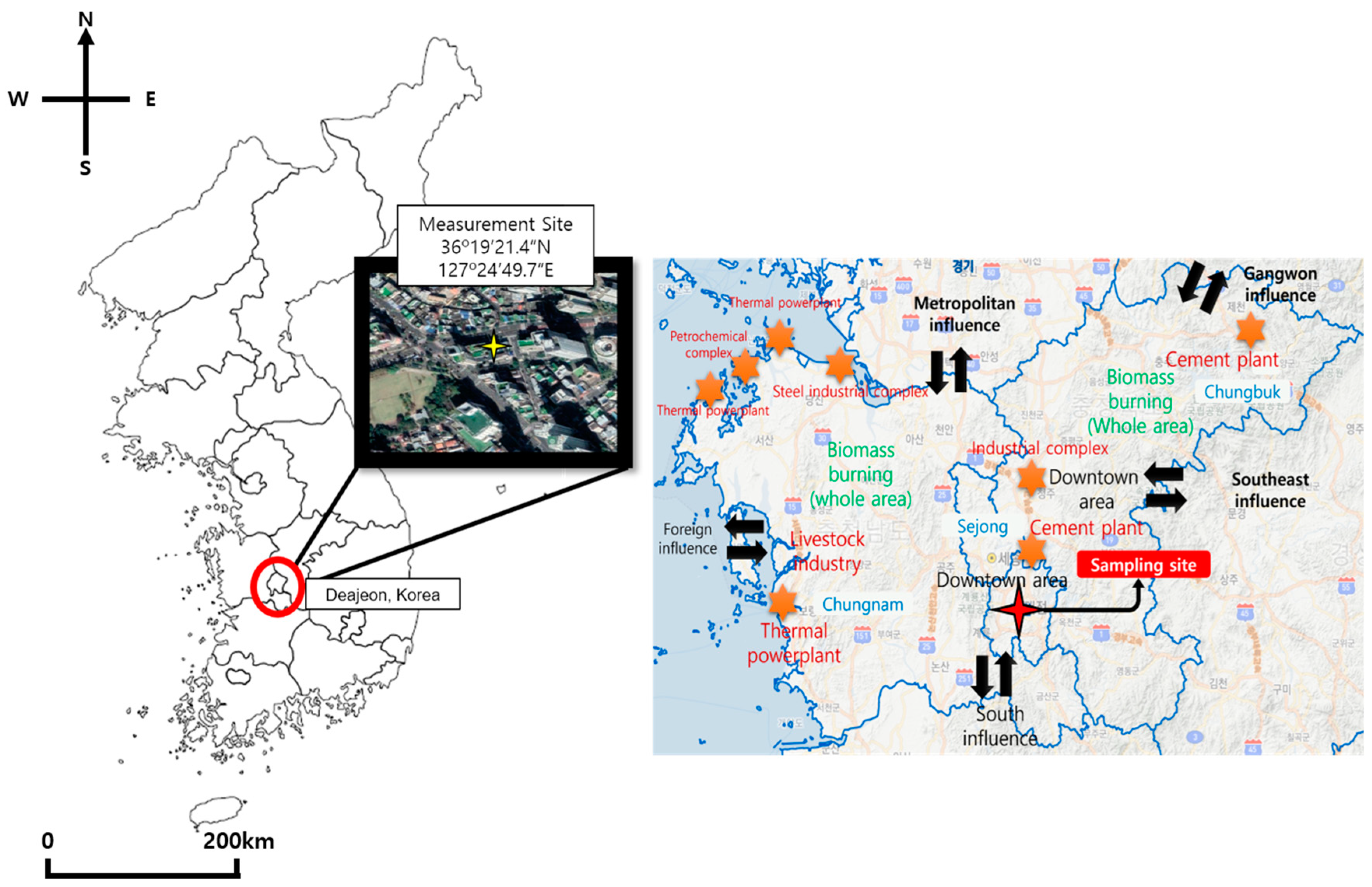
2.1. Sampling Location and Monitoring Site
2.2. Sampling and Data Analysis
2.3. Positive Matrix Factorization (PMF)
2.4. Emission Inventories
2.5. Advanced Concentration, Emission, and Retention Time-Weighted Trajectory (ACERWT)
3. Results and Discussions
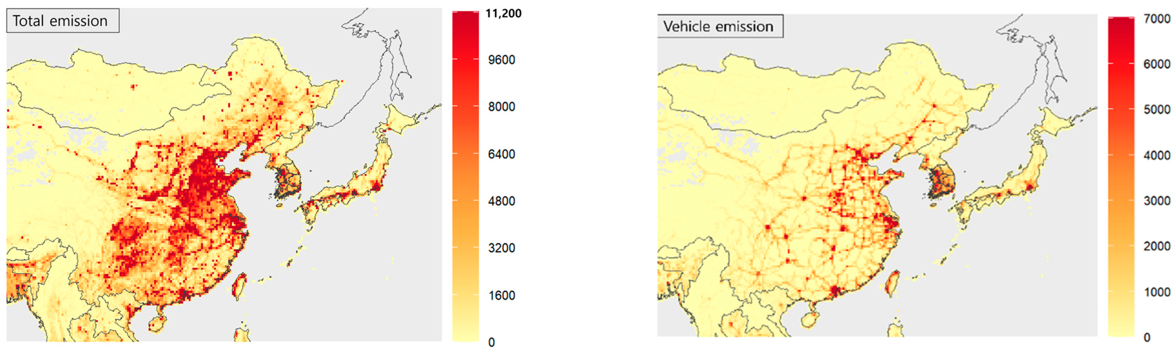
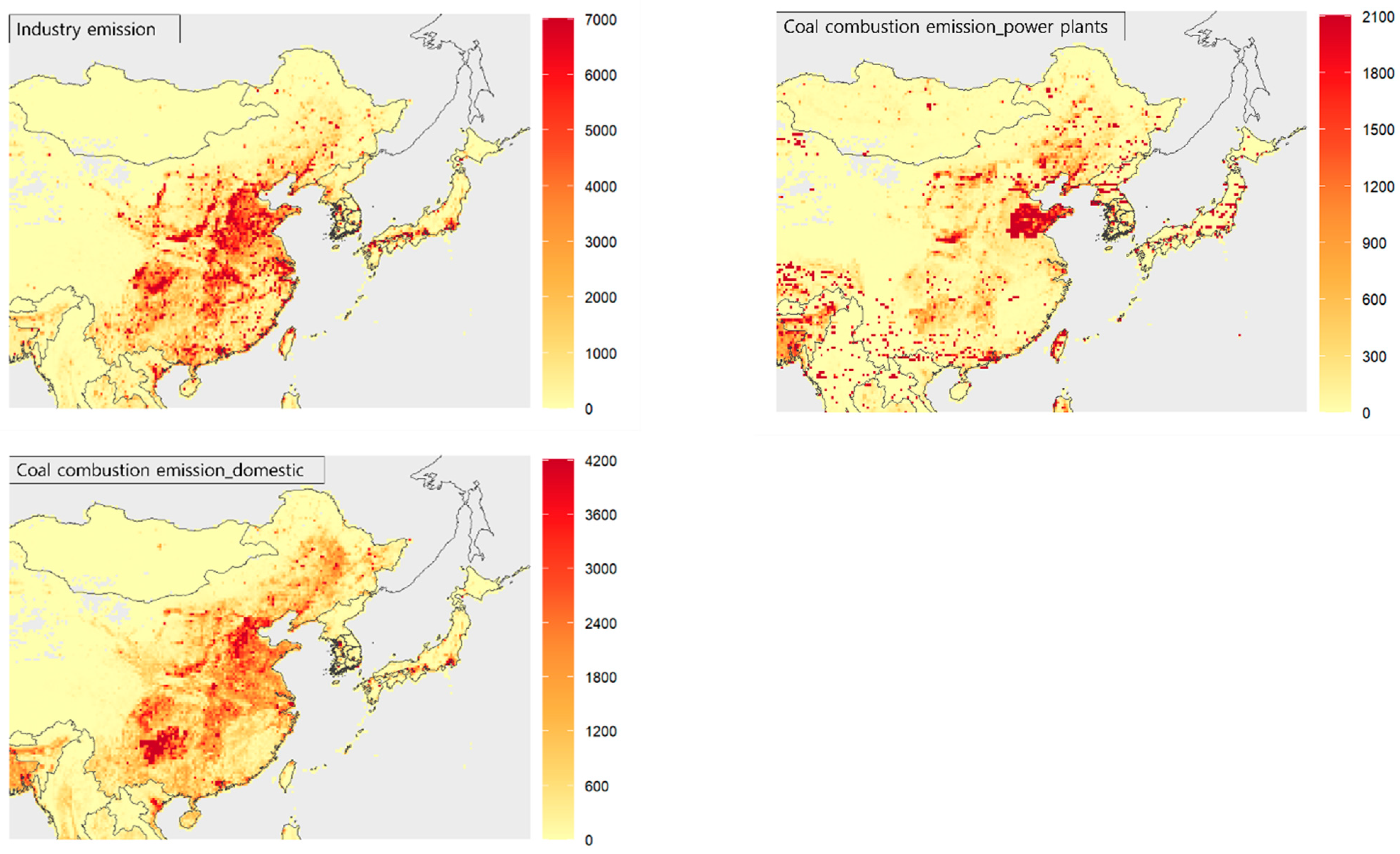
3.1. Emission Inventory
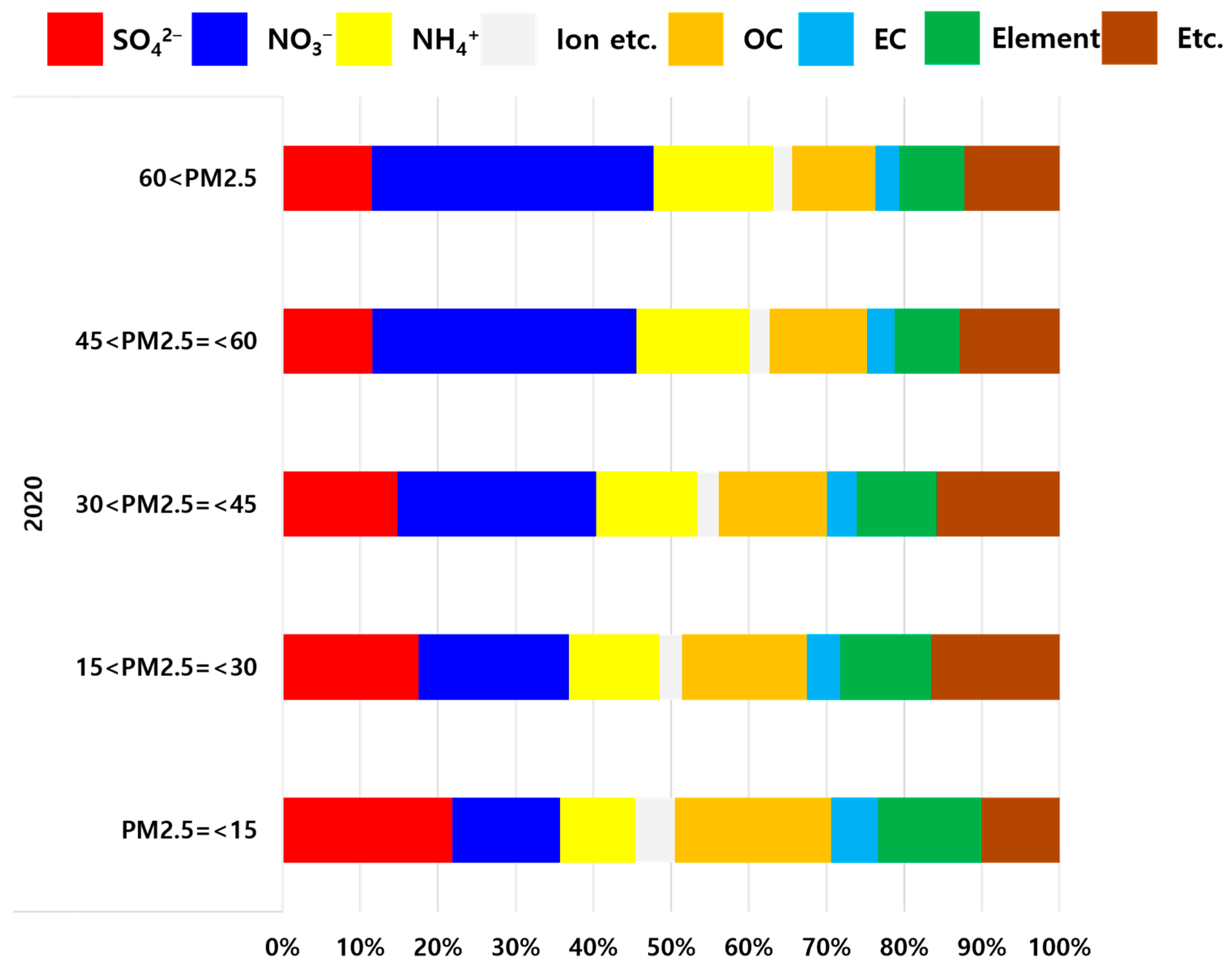
3.2. Chemical Composition of PM2.5
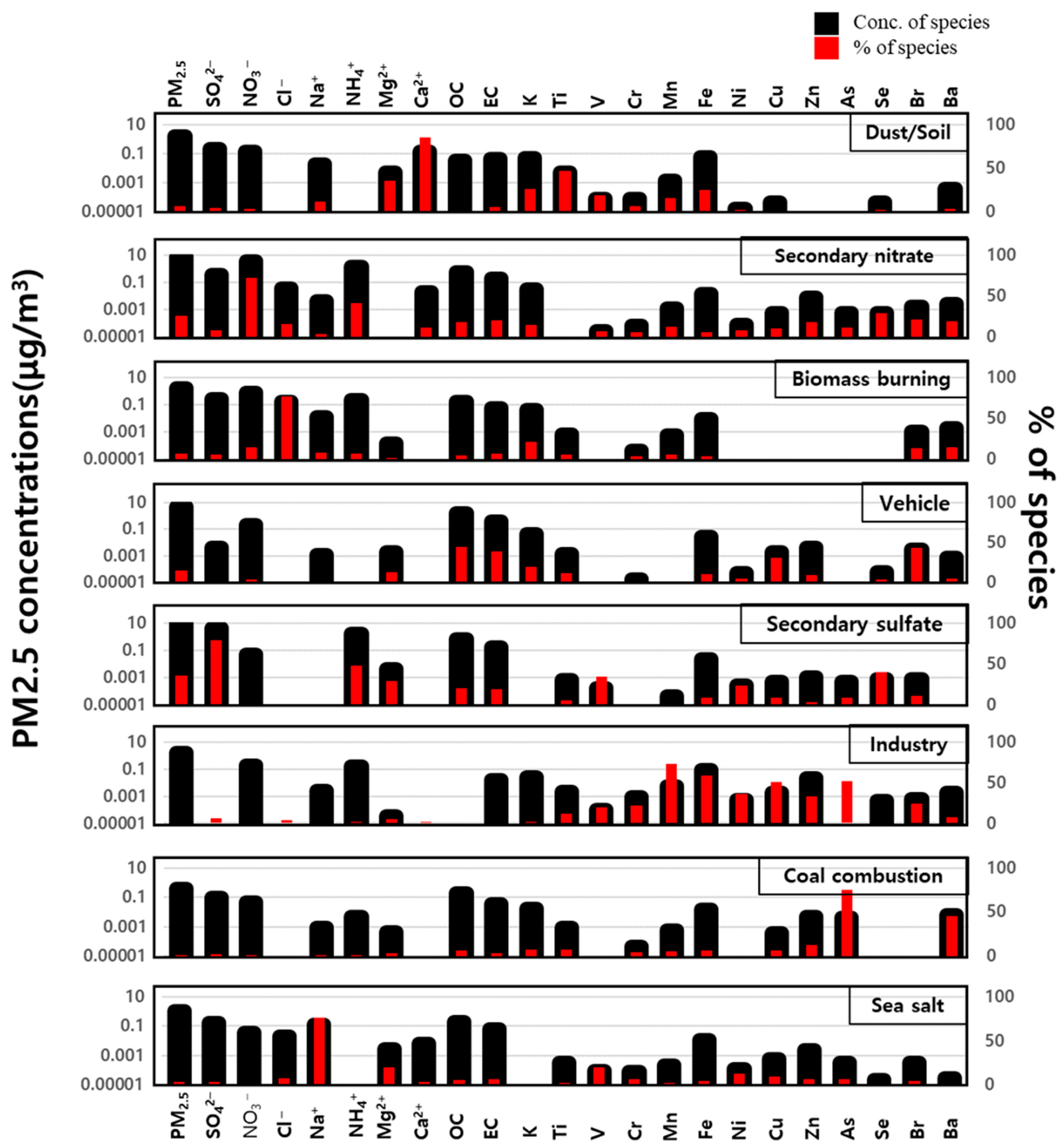
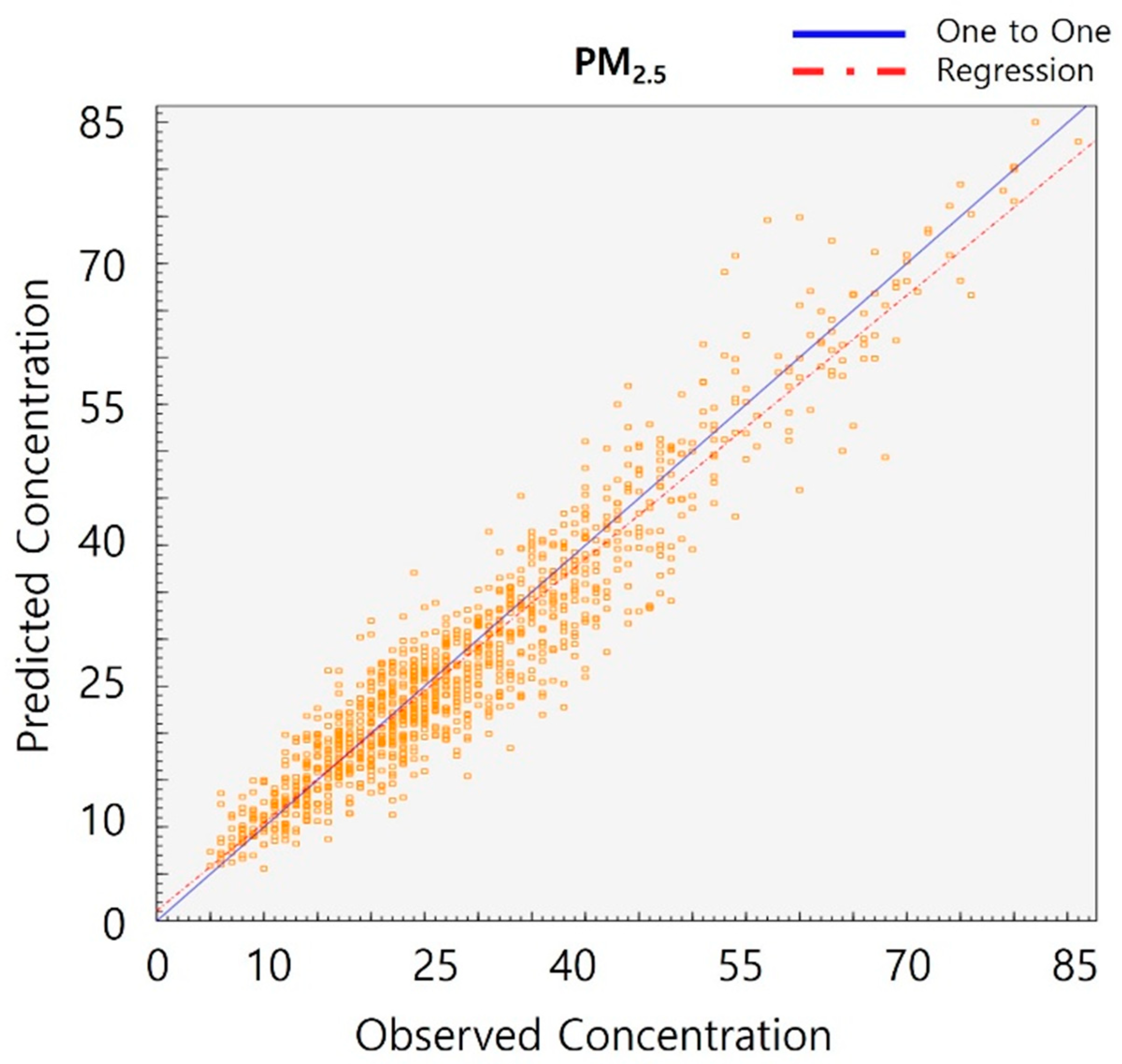
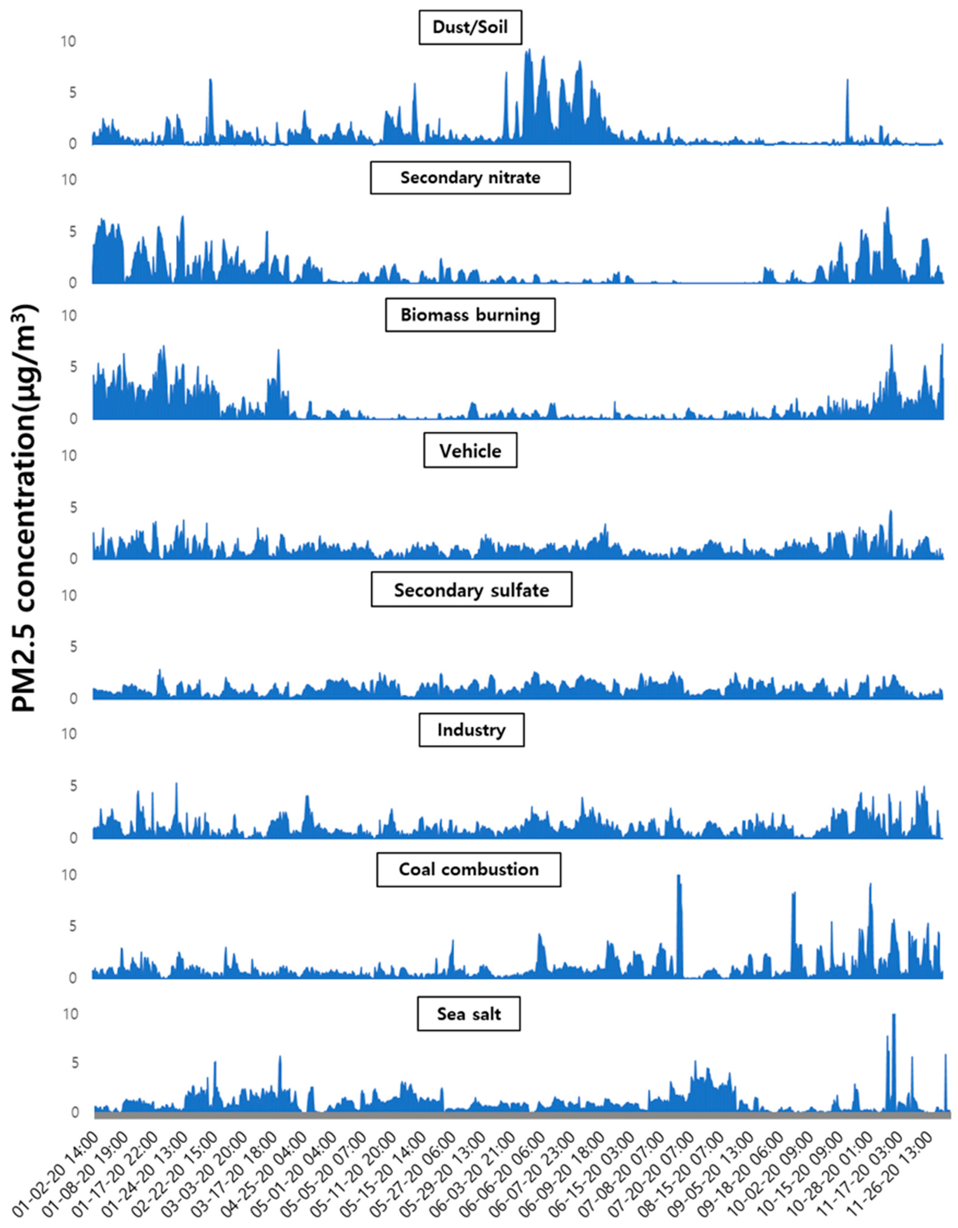
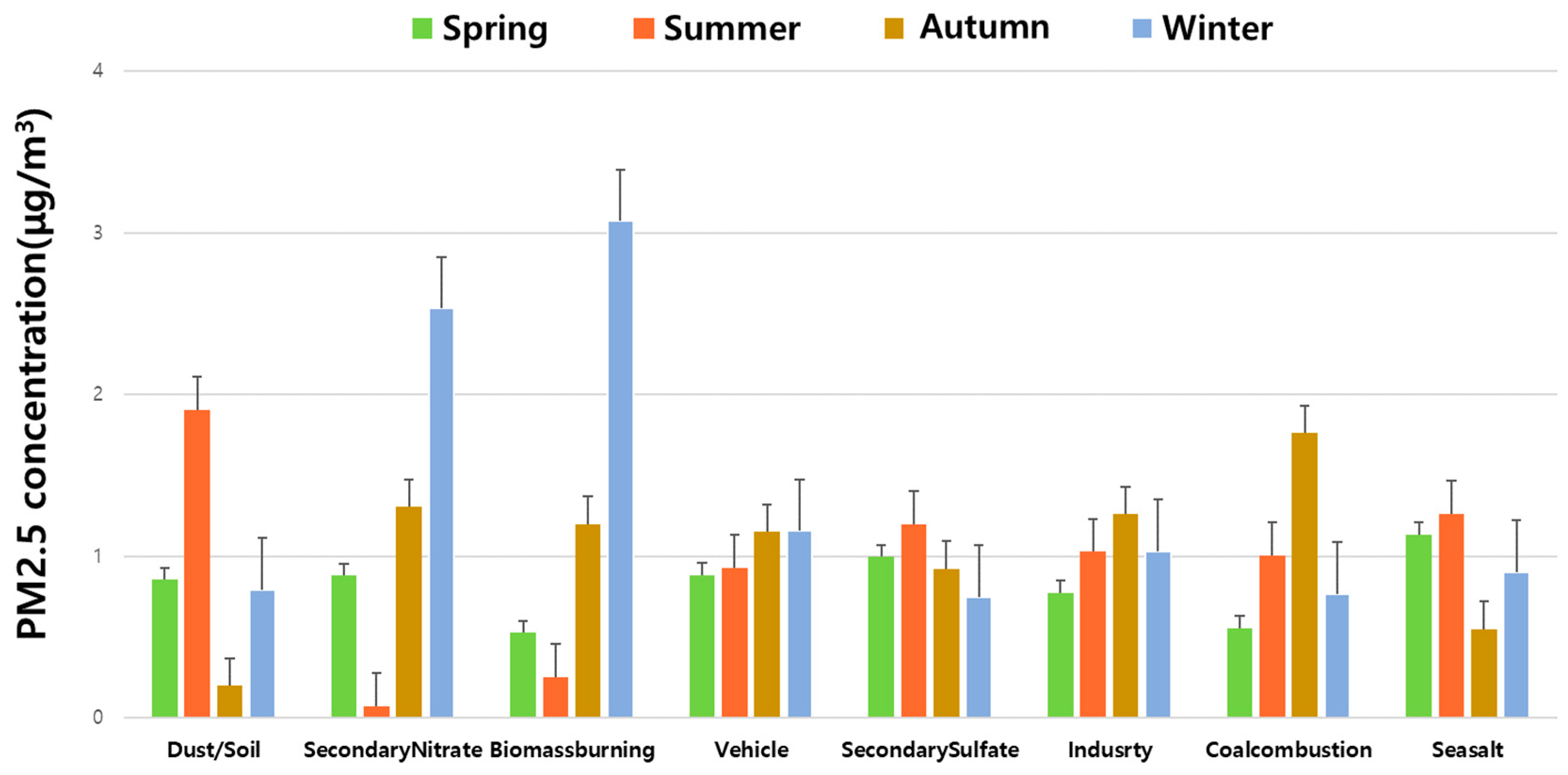
3.3. Source Apportionment Using PMF Receptor Model
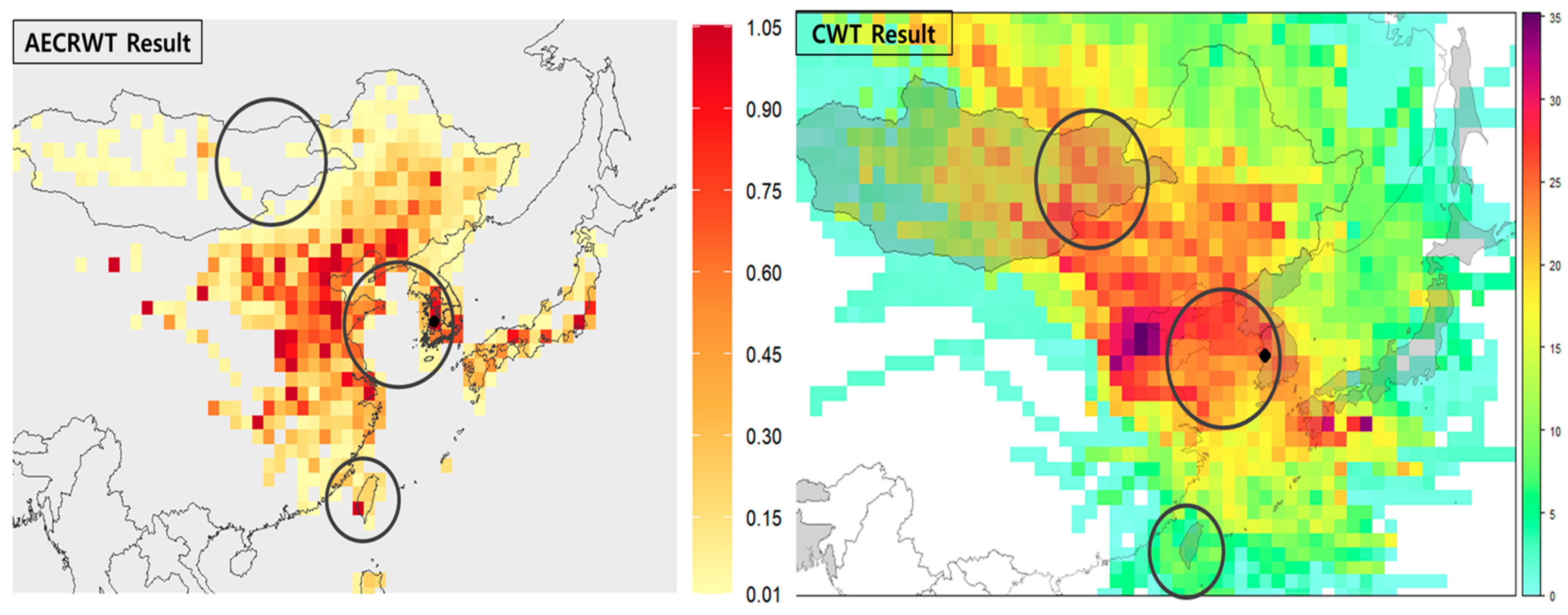
3.4. Results of the Regional Contributions by ACERWT
4. Conclusions
Author Contributions
Funding
Institutional Review Board Statement
Informed Consent Statement
Data Availability Statement
Acknowledgments
Conflicts of Interest
References
- Jung, E.M.; Kim, K.N.; Park, H.; Shin, H.H.; Kim, H.S.; Cho, S.J.; Kim, S.T.; Ha, E.H. Association between prenatal exposure to PM2.5 and the increased risk of specified infant mortality in South Korea. Environ. Int. 2020, 144, 105997. [Google Scholar] [CrossRef]
- Han, J.S.; Moon, K.J.; Kim, Y.J. Identification of potential sources and source regions of fine ambient particles measured at Gosan background site in Korea using advanced hybrid receptor model combined with positive matrix factorization. J. Geophys. Res. 2006, 111, D22217. [Google Scholar] [CrossRef]
- Hwang, I.J.; Kim, D.S. Research trends of receptor models in Korea and Foreign Countries and Improvement Directions for Air Quality Management. J. Korean Soc. Atmos. Environ. 2013, 29, 459–476. [Google Scholar] [CrossRef]
- Miller, M.S.; Friedlander, S.K.; Hidy, G.M. A chemical element balance for the Pasadena aerosol. J. Colloid Interface Sci. 1972, 39, 165–176. [Google Scholar] [CrossRef]
- Paatero, P. Least squares formulation of robust non-negative factor analysis. Chemom. Intell. Lab. Syst. 1997, 37, 23–35. [Google Scholar] [CrossRef]
- Reff, A.; Eberly, S.I.; Bhave, P.V. Receptor modeling of ambient particulate matter data using positive matrix factorization: Review of existing methods. J. Air Waste Manag. Assoc. 2007, 57, 146–154. [Google Scholar] [CrossRef]
- Hwang, I.; Hopke, P.K. Estimation of source apportionment and potential source locations of PM2.5 at a west coastal IMPROVE site. Atmos. Environ. 2007, 41, 506–518. [Google Scholar] [CrossRef]
- Thurston, G.D.; Ito, K.; Lall, R. A source apportionment of U.S. fine particulate matter air pollution. Atmos. Environ. 2011, 45, 3924–3936. [Google Scholar] [CrossRef]
- Belis, C.A.; Karagulian, F.; Larsen, B.R.; Hopke, P.K. Critical review and meta-analysis of ambient particulate matter source apportionment using receptor models in Europe. Atmos. Environ. 2013, 69, 94–108. [Google Scholar] [CrossRef]
- Lu, Z.J.; Liu, Q.Y.; Xiong, Y.; Huang, F.; Zhou, J.B.; Schauer, J.J. A hybrid source apportionment strategy using positive matrix factorization (PMF) and molecular marker chemical mass balance (MM-CMB) models. Environ. Pollut. 2018, 238, 39–51. [Google Scholar] [CrossRef]
- Park, M.B.; Lee, T.J.; Lee, E.S.; Kim, D.S. Enhancing source identification of hourly PM2.5 data in Seoul based on a dataset segmentation scheme by positive matrix factorization (PMF). Atmos. Pollut. Res. 2019, 10, 1042–1059. [Google Scholar] [CrossRef]
- Park, J.E.; Kim, H.W.; Kim, Y.K.; Heo, J.B.; Kim, S.W.; Jeon, K.H.; Yi, S.M.; Hopke, P.K. Source apportionment of PM2.5 in Seoul, South Korea and Beijing, China using dispersion normalized PMF. Sci. Total Environ. 2022, 833, 155056. [Google Scholar] [CrossRef]
- Hopke, P.K.; Gao, N.; Cheng, M.D. Combining chemical and meteorological data to infer source areas of airborne pollutants. Chemom. Intell. Lab. Syst. 1993, 19, 187–199. [Google Scholar] [CrossRef]
- Seibert, P.; Kromp-Kolb, H.; Baltensperger, U.; Jost, D.T.; Schwikowski, M.; Kasper, A.; Puxbaum, H. Trajectory analysis of aerosol measurements at high Alpine sites. In Transport and Transformation of Pollutants in the Troposphere; Borrell, P.M., Ed.; Elsevier: New York, NY, USA, 1994; Volumes 689–693. [Google Scholar]
- Stohl, A. Trajectory statistics—A new method to establish sourcereceptor relationships of air pollutants and its application to the transport of particulate sulfate in Europe. Atmos. Environ. 1996, 30, 579–587. [Google Scholar] [CrossRef]
- Han, Y.J.; Holsen, T.M.; Hopke, P.K.; Cheong, J.P.; Kim, H.; Yi, S.M. Identification of source locations for atmospheric dry deposition of heavy metals during yellow-sand events in Seoul, Korea in 1998 using hybrid receptor models. Atmos. Environ. 2004, 38, 5353–5361. [Google Scholar] [CrossRef]
- Lupu, A.; Maenhaut, W. Application and comparison of two statistical trajectory techniques for identification of source regions of atmospheric aerosol species. Atmos. Environ. 2002, 36, 5607–5618. [Google Scholar] [CrossRef]
- Fan, W.; Qin, K.; Xu, J.; Yuan, L.; Li, D.; Jin, Z.; Zhang, K. Aerosol vertical distribution and sources estimation at a site of the Yangtze River Delta region of China. Atmos. Res. 2019, 217, 128–136. [Google Scholar] [CrossRef]
- Dimitriou, K.; Mihalopoulos, N.; Leeson, S.R.; Twigg, M.M. Sources of PM2.5-bound water soluble ions at EMEP’s Auchencorth Moss (UK) Supersite revealed by 3D-Concentration Weighted Trajectory (CWT) model. Chemosphere 2021, 274, 129979. [Google Scholar] [CrossRef]
- Wang, Y.Q.; Zhang, X.Y.; Arimoto, R. The contribution from distant dust sources to the atmospheric particulate matter loadings at XiAn, China during spring. Sci. Total Environ. 2006, 368, 875–883. [Google Scholar] [CrossRef]
- Jeong, U.K.; Kim, J.H.; Lee, H.L.; Jung, J.S.; Kim, Y.J.; Song, C.H.; Koo, J.H. Estimation of the contributions of long range transported aerosol in East Asia to carbonaceous aerosol and PM concentrations in Seoul, Korea using highly time resolved measurements: A PSCF model approach. J. Environ. Monit. 2011, 13, 1905–1918. [Google Scholar] [CrossRef]
- Zachary, M.; Yin, L.; Zacharia, M. Application of PSCF and CWT to Identify Potential Sources of Aerosol Optical Depth in ICIPE Mbita. Open Access Libr. J. 2018, 5, e4487. [Google Scholar] [CrossRef]
- Do, W.G.; Jung, W.S. Estimation of PM10 source locations in Busan using PSCF model. J. Environ. Sci. Int. 2015, 24, 793–806. [Google Scholar] [CrossRef]
- Han, S.; Joo, H.; Song, H.; Lee, S.; Han, J. Source apportionment of PM2.5 in Daejeon metropolitan region during January and May to June, 2021 in Korea using a hybrid receptor model. Atmosphere 2022, 13, 1902. [Google Scholar] [CrossRef]
- National Institute of Environmental Research (NIER). Annual Report of Intensive Air Quality Monitoring Station; NIER: Incheon, Republic of Korea, 2020; NIER-GP2020–2208. [Google Scholar]
- Nuhoglu, Y.; Yazici, M.; Nuhoglu, C.; Kam, E.; Adar, E.; Kuzu, L.; Osmanlioglu, A.E. XRF Analysis of Airborne Heavy Metals and Distribution of Environment in Sivas City Turkey through Dust Samples. In Proceedings of the EurAsia Waste Management Symposium, Istanbul, Turkey, 26–28 October 2020; pp. 26–28. [Google Scholar]
- National Institute of Environmental Research (NIER). Establishment of Guidelines for the PMF Modeling and Applications; NIER: Incheon, Republic of Korea, 2020; NIER-SP2020–2273. [Google Scholar]
- Kurokawa, J.; Ohara, T. Long-Term Historical Trends in Air Pollutant Emissions in Asia: Regional Emission Inventory in Asia (REAS) version 3. Atmos. Chem. Phys. 2020, 20, 12761–12793. [Google Scholar] [CrossRef]
- Guo, S.; Hu, M.; Wang, Z.B.; Slanina, J.; Zhao, Y.L. Size-resolved aerosol water-soluble ionic compositions in the summer of Beijing: Implication of regional secondary formation. Atmos. Chem. Phys. 2010, 10, 947–959. [Google Scholar] [CrossRef]
- National Research Foundation of Korea (NRF). A study on the physicochemical properties and formation mechanism considering the characteristics of domestic and foreign influences of fine particles in the central area. In Fine Particle Reseach Initiative in East Asian Considering National Differences (FRIEND) Project, 2020MG1A1114999; National Research Foundation of Korea (NRF): Daejeon, Republic of Korea, 2022. [Google Scholar]
- Hwang, I.J.; Yi, S.M.; Park, J.S. Estimation of Source Apportionment for Filter-based PM2.5 Data using the EPA-PMF Model at Air Pollution Monitoring Supersites. J. Korean Soc. Atmos. Environ. 2020, 36, 620–632. [Google Scholar] [CrossRef]
- Taghvaee, S.; Sowlat, M.H.; Mousavi, A.; Hassanvand, M.S.; Yunesian, M.; Naddafi, K.; Sioutas, C. Source apportionment of ambient PM2.5 in two locations in central Tehran using the Positive Matrix Factorization (PMF) model. Sci. Total Environ. 2018, 628–629, 672–686. [Google Scholar] [CrossRef]
- Chun, M.Y.; Lee, Y.J.; Kim, H.K. Concentration of NH4NO3 in TSP in Seoul Ambient Air. J. Korean Soc. Atmos. Environ. 1994, 10, 130–136. [Google Scholar]
- Bayramoğlu Karşı, M.B.; Berberler, E.; Berberler, T.; Aslan, Ö.; Yenisoy-Karakaş, S.; Karakaş, D. Correction and source apportionment of vehicle emission factors obtained from Bolu Mountain Highway Tunnel, Turkey. Atmos. Pollut. Res. 2020, 11, 2133–2141. [Google Scholar] [CrossRef]
- Hao, Y.; Gao, C.; Deng, S.; Yuan, M.; Song, W.; Lu, Z.; Qiu, Z. Chemical characterisation of PM2.5 emitted from motor vehicles powered by diesel, gasoline, natural gas, and methanol fuel. Sci. Total Environ. 2019, 674, 128–139. [Google Scholar] [CrossRef]
- Coufalík, P.; Matoušek, T.; Křůmal, K.; Vojtíšek-Lom, M.; Beránek, V.; Mikuška, P. Content of metals in emissions from gasoline, diesel, and alternative mixed biofuels. Environ. Sci. Pollut. Res. Int. 2019, 26, 29012–29019. [Google Scholar] [CrossRef]
- Cheung, K.L.; Ntziachristos, L.; Tzamkiozis, T.; Schauer, J.J.; Samaras, Z.; Moore, K.F.; Sioutas, C. Emissions of particulate trace elements, metals and organic species from gasoline, diesel, and biodiesel passenger vehicles and their relation to oxidative potential. Aerosol Sci. Technol. 2010, 44, 500–513. [Google Scholar] [CrossRef]
- Dockery, D.W.; Stone, P.H. Cardiovascular risks from fine particulate air pollution. N. Engl. J. Med. 2007, 356, 511–513. [Google Scholar] [CrossRef]
- Son, S.E.; Park, S.S.; Bae, M.A.; Kim, S.T. A study on characteristics of high pollution observed around large scale stationary sources in Chungcheongnam-do province. J. Korean Soc. Atmos. Environ. 2020, 36, 669–687. [Google Scholar] [CrossRef]
- Gonçalves, S.J.; Weis, J.; China, S.; Evangelista, H.; Harder, T.H.; Müller, S.; Sampaio, M.; Laskin, A.; Gilles, M.K.; Godoi, R.H.M. Photochemical reactions on aerosols at West Antarctica: A molecular case-study of nitrate formation among sea salt aerosols. Sci. Total Environ. 2021, 758, 143586. [Google Scholar] [CrossRef]
- Filonchyk, M.; Peterson, M. Development, progression, and impact on urban air quality of the dust storm in Asia in March 15–18, 2021. Urban Clim. 2022, 41, 101080. [Google Scholar] [CrossRef]
- Li, Y.; Lin, T.; Hu, L.; Feng, J.; Guo, Z. Time trends of polybrominated diphenyl ethers in east China seas: Response to the booming of PBDE pollution industry in China. Environ. Int. 2016, 92–93, 507–514. [Google Scholar] [CrossRef]
- Garcia Novo, P.; Kyozuka, Y. Tidal stream energy as a potential continuous power producer: A case study for west Japan. Energy Convers. Manag. 2021, 245, 114533. [Google Scholar] [CrossRef]


| Program Activity | Carrier Gas | Ramp Time (Second) | Program Temperature |
|---|---|---|---|
| Oven Purge | Helium | 10 | 1 |
| 1stRamp | Helium | 70 | 310 |
| 2edRamp | Helium | 60 | 480 |
| 3rdRamp | Helium | 60 | 615 |
| 4thRamp | Helium | 90 | 840 |
| - | Helium | 30 | 0 |
| 1stRamp | O2/Helium | 35 | 550 |
| 2ndRamp | O2/Helium | 105 | 850 |
| Internal Std. Calibration | CH4/Helium | 120 | 0 |
| Cool down | Helium | 1 | 0 |
| Components | MDL | Components | MDL | Components | MDL | ||
|---|---|---|---|---|---|---|---|
| Ions | SO42− | 0.00595 | Elements | Si | 0.03690 | Cu | 0.00022 |
| NO3− | 0.01018 | S | 0.00515 | Zn | 0.00019 | ||
| Cl− | 0.00966 | K | 0.00309 | As | 0.00016 | ||
| Na+ | 0.00328 | Ca | 0.00069 | Se | 0.00021 | ||
| NH4+ | 0.00218 | Ti | 0.00036 | Br | 0.00025 | ||
| K+ | 0.04444 | V | 0.00034 | Ba | 0.00088 | ||
| Mg2+ | 0.00106 | Cr | 0.00025 | Pb | 0.00030 | ||
| Ca2+ | 0.00286 | Mn | 0.00032 | ||||
| Carbons | OC | 0.29731 | Fe | 0.00042 | |||
| EC | 0.00084 | Ni | 0.00024 |
| AVG. | MAX. | MIN. | STD. | Sample No. | |
|---|---|---|---|---|---|
| PM2.5 | 22.1 | 104 | 1 | 15.4 | 8460 |
| SO42− | 3.75 | 15.9 | 0.06 | 2.47 | 6244 |
| NO3− | 5.52 | 46.5 | 0.01 | 6.42 | 6258 |
| Cl− | 0.31 | 5.07 | 0.01 | 0.35 | 6257 |
| Anion | 9.56 | 58.2 | 0.11 | 7.92 | 8693 |
| Anion/PM2.5 | 0.38 | 0.81 | 0.06 | 0.20 | 8693 |
| Na+ | 0.15 | 2.62 | 0.01 | 0.17 | 6255 |
| NH4+ | 2.91 | 17.9 | 0.01 | 2.55 | 6258 |
| K+ | 0.15 | 1.14 | 0.01 | 0.12 | 6050 |
| Mg2+ | 0.02 | 0.95 | 0.01 | 0.04 | 6218 |
| Ca2+ | 0.11 | 2.27 | 0.01 | 0.15 | 6223 |
| Cation | 3.30 | 18.2 | 0.05 | 2.67 | 8693 |
| Cation/PM2.5 | 0.002 | 0.07 | 0.0001 | 0.006 | 8785 |
| Ion/PM2.5 | 0.51 | 0.99 | 0.04 | 0.27 | 8693 |
| OC | 3.42 | 16.1 | 0.27 | 2.05 | 7367 |
| EC | 0.95 | 4.69 | 0.02 | 0.58 | 7367 |
| Carbon | 4.38 | 19.2 | 0.46 | 2.85 | 8744 |
| Carbon/PM2.5 | 0.22 | 0.97 | 0.04 | 0.12 | 8744 |
| Metal | 2.41 | 10.4 | 0.06 | 1.66 | 8780 |
| Metal/PM2.5 | 0.12 | 0.86 | 0.01 | 0.06 | 8780 |
| Period | Season | PM2.5 ≤ 15 | 15 < PM2.5 ≤ 30 | 30 < PM2.5 ≤ 45 | 45 < PM2.5 ≤ 60 | 60 < PM2.5 |
|---|---|---|---|---|---|---|
| 1~2, 12.2020 | Winter | 560 | 748 | 480 | 230 | 165 |
| 3~5.2020 | Spring | 690 | 1027 | 355 | 82 | 23 |
| 6~8.2020 | Summer | 1180 | 633 | 247 | 17 | 1 |
| 9~11.2020 | Autumn | 986 | 679 | 229 | 76 | 52 |
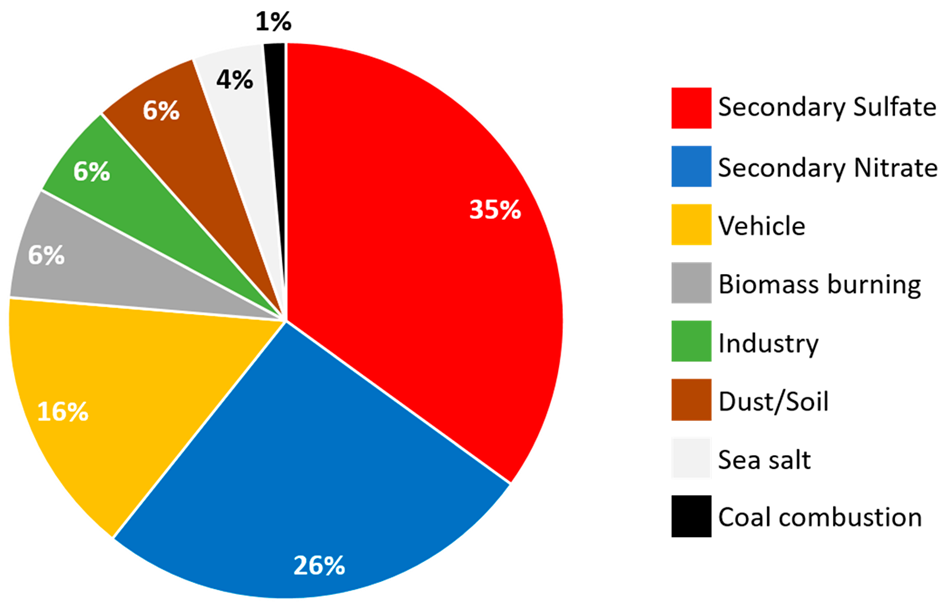
| Source | Contribution |
|---|---|
| Secondary Sulfate | 35% |
| Secondary Nitrate | 26% |
| Vehicle | 16% |
| Biomass burning | 6% |
| Industry | 6% |
| Dust/soil | 6% |
| Sea salt | 4% |
| Coal combustion | 1% |
| Pie chart | |
 | |
Disclaimer/Publisher’s Note: The statements, opinions and data contained in all publications are solely those of the individual author(s) and contributor(s) and not of MDPI and/or the editor(s). MDPI and/or the editor(s) disclaim responsibility for any injury to people or property resulting from any ideas, methods, instructions or products referred to in the content. |
© 2024 by the authors. Licensee MDPI, Basel, Switzerland. This article is an open access article distributed under the terms and conditions of the Creative Commons Attribution (CC BY) license (https://creativecommons.org/licenses/by/4.0/).
Share and Cite
Han, S.-w.; Joo, H.-s.; Kim, K.-c.; Cho, J.-s.; Moon, K.-j.; Han, J.-s. Modification of Hybrid Receptor Model for Atmospheric Fine Particles (PM2.5) in 2020 Daejeon, Korea, Using an ACERWT Model. Atmosphere 2024, 15, 477. https://doi.org/10.3390/atmos15040477
Han S-w, Joo H-s, Kim K-c, Cho J-s, Moon K-j, Han J-s. Modification of Hybrid Receptor Model for Atmospheric Fine Particles (PM2.5) in 2020 Daejeon, Korea, Using an ACERWT Model. Atmosphere. 2024; 15(4):477. https://doi.org/10.3390/atmos15040477
Chicago/Turabian StyleHan, Sang-woo, Hung-soo Joo, Kyoung-chan Kim, Jin-sik Cho, Kwang-joo Moon, and Jin-seok Han. 2024. "Modification of Hybrid Receptor Model for Atmospheric Fine Particles (PM2.5) in 2020 Daejeon, Korea, Using an ACERWT Model" Atmosphere 15, no. 4: 477. https://doi.org/10.3390/atmos15040477
APA StyleHan, S.-w., Joo, H.-s., Kim, K.-c., Cho, J.-s., Moon, K.-j., & Han, J.-s. (2024). Modification of Hybrid Receptor Model for Atmospheric Fine Particles (PM2.5) in 2020 Daejeon, Korea, Using an ACERWT Model. Atmosphere, 15(4), 477. https://doi.org/10.3390/atmos15040477