Abstract
The incoming solar radiation arriving the Earth’s surface is strongly influenced by surface terrain. Conventional global weather forecast models, with grid scales of about 10 km, lack the resolution to accurately capture terrain-induced variations. We devised a new parameterization method to incorporate high-resolution subgrid-scale terrain data into grid-scale radiative flux calculations without averaging or smoothing topographic features. Utilizing a 15″ digital elevation model from the Shuttle Radar Topography Mission, we computed subgrid-scale data and transformed them onto the Korean Integrated Model’s cubed sphere grid using a Voronoi diagram to maintain geographical accuracy. The new scheme was initially evaluated through offline ideal tests and case studies. The results demonstrated that the scheme accurately captured the variations in downward shortwave flux, keeping the mean flux on a global scale nearly constant. The global mean flux difference in all skies was less than 0.01%. Statistical analyses demonstrated improved temperature and geopotential height predictions compared to reanalysis data. The anomaly correlation coefficient for East Asia at 850 hPa increased by 0.036 at 240 forecast hours. Overall, the anomaly correlation coefficient and root mean square error of geopotential height and temperature showed enhancements, particularly in the Northern Hemisphere and tropics. Importantly, the scheme introduces negligible additional memory and CPU requirements, making it suitable for both regional and global models. Only a 0.58% increase in CPU time was observed for the 10-day forecast.
1. Introduction
Surface radiation can be strongly influenced by the topological features of mountainous terrains. Ref. [1] analyzed the surface radiation budget in an alpine valley and showed that incoming direct solar radiation can differ by approximately 200 Wm−2 at different sites in the valley, with a phase lag in the diurnal cycle. The sloping terrain modifies the solar incidence angle. Direct solar radiation can be greatly increased even when the solar elevation is near the horizon during sunset or sunrise. Shading is also an important factor determining the final arrival flux at the surface. The side of the mountain opposite the sun is self-shadowed, blocking direct radiation. Ref. [2] investigated the magnitude and causes of spatial variability in surface radiative fluxes in a complex alpine landscape using a surface radiation budget model. They found that, in order of importance, the characteristics that influencing flux variability were the slope aspect, slope angle, elevation, albedo, shading, sky view factor, and leaf area index. We implemented the subgrid topographic radiative effect on a numerical weather forecasting model, focusing on the following main characteristics: slope aspect, slope angle, and self-shading of solar direct radiation. In terms of weather and climate, uneven solar radiation reaching the ground due to topology is essential for predictive improvement. Additionally, predicting such variability in solar radiation has various agricultural applications [3].
A number of works have been conducted on subgrid-scale topographic effects on solar radiation. Ref. [4] incorporated the terrain effect on radiation into the National Oceanic Atmosphere Administration/National Centers for Environmental Protection Non-Hydrostatic Mesoscale Model. They introduced a sub-grid scale correction factor and nonlocal sky view factor to the downward flux of a model grid cell. In order to optimize computational resources during model execution, correction factors are calculated diagnostically for each hour of the model run period in advance of the actual model execution. They showed that the parametrization improved 2 m temperature forecasts over the Alps. Furthermore, refs. [5,6] also implemented the topographic effect parameterized in the High-Resolution Limited Area Model, based on the approach proposed by [4]. They processed high-resolution orography data to incorporate the impact of topography. Ref. [7] introduced a scheme in the Met Office Unified Model, which conserves energy over an extended region where the mean flux into the surface is independent of resolution. The first- and second-order surface topography, including its interaction with the surrounding terrain, is applied for both solar and thermal radiation. Ref. [8] implemented a grid and subgrid-scale radiation parameterization for the mesoscale Weather Forecast Model with the immersed boundary method, which uses a nonconforming grid and represents the topography by imposing boundary conditions along an immersed terrain surface. A subgrid terrain radiative forcing scheme is also implemented in the Regional Climate Model Version 4.1 by [9]. The scheme primarily considers slope effect on both solar and thermal radiation and has been tested over the Tibetan Plateau.
All of the aforementioned previous works were conducted at the regional scale. Ref. [10] proposed an efficient method that can be applied to global climate models, utilizing 3D Monte Carlo photon tracing simulations. They developed a parameterization scheme that employs a set of multiple linear regression equations to relate the subgrid terrain effects to the domain-averaged topographic factors. Their method has been implemented to regional and global model; in the Weather Research and Forecasting model [11,12], Community Land Model [13], Taiwan Earth System Model [14], and Energy Exascale Earth System Model Land Model [15].
The most challenging aspect of applying high-resolution topological data to an NWP model is the computational cost. The schemes described by [4] and [6] do not require an additional large computational cost but the coefficients must be pre-calculated prior to each forecast run for all periods in the forecasting time. Here, we introduce a new scheme with the subgrid-scale slope factor as defined in [4] that can be applied to NWP with negligible computational memory and CPU usage. This scheme can be used not only for the limited-area model but also for the global model. However, as a compromise for the application in operational global models, the topographic terrain effect is selectively applied on certain criteria, where the mean flux on a global scale remains nearly constant. We introduce our scheme and describe how it is applied in a cubed sphere grid earth system in the following sections. Subsequently, we discuss the caveats and limitations associated with the scheme.
2. Methods
Ref. [16] introduced a basic theory describing the effect of slope on direct solar radiation. Direct solar flux arriving at a slope in a certain direction is determined by multiplying the flux by the cosine of the angle n between the direction of the sun rays and the normal of the slope surface:
where is the slope height angle, the solar height angle, is the solar azimuth angle, and the slope aspect angle. Ref. [4] introduced a slope factor, , that modifies the arriving direct solar radiation by considering the area of a sloping surface by a factor . The final downward direct solar flux (assuming no shading is present) is given by:
The slope factor can be decomposed into two parts: solar-related and topography-related variables. If we define and , the slope factor of Equation (2) can be rewritten as:
Because the and terms are computed using topography-related variables , ), they can be considered as constant fields. These terms are precomputed only once and can then be input to the NWP for any starting forecasting time and period. However, the solar-related variables and cannot be precomputed because they depend on the running time of the NWP. Two issues can arise when applying this method. The first is resolution; solar-related variables are computed in a model grid, typically with a resolution of a few kilometers in the case of global circulation models. However, topographic data have a much higher resolution of at least a few hundred meters. If these data are averaged at the model grid scale, all topographic information is smoothed, and their effect becomes negligible. Although the radiation fluxes should be averaged, the orography should not be smoothed. The average flux in a model grid over N topographic data (i.e., subgrid) can be expressed as follows:
where and . As shown in Equation (4), the solar-related variables and are constant over the model grid; thus, the summation applies only to topography-related variables. Using this approach, the averaged flux can be obtained over N subgrids without smoothing the orography. Another issue arises when the term becomes negative (/2 < < ). This case occurs at the self-shielded face of a mountain, where the sun ray arrives on the opposite side. If some subgrids in a model grid are self-shielded, the slope factor becomes negative, resulting in an incorrectly averaged flux . The negative flux of the self-shield subgrids should not be counted on because all direct radiation components are blocked out. However, the sign of the slope factor depends on both the solar position and slope direction, and thus cannot be predicted before running the NWP model. A negative slope factor typically occurs at low solar altitudes in deep valleys where other characteristics are also important, such as shadows from the surrounding terrain and sky views. As a conservative approach, to ensure that all subgrid slope factors are positive, we applied the radiative topographic effect when the average slope of the model grid was smaller than the solar height angle.
Thus, the A, B, and C coefficients defined above for each grid point of the NWP were pre-computed and provided as ancillary data.
3. Topographic Data
High-resolution topographic data, the slope height angle , and the slope aspect angle , were produced from the Digital Elevation Model (DEM) of the Shuttle Radar Topography Mission (SRTM). The SRTM project ([17]) was a joint endeavor of National Aeronautics and Space Administration, the National Geospatial-Intelligence Agency, and the German and Italian Space Agencies and flew in February 2000. It produced the most complete, high-resolution (at 1 arcsec resolution) digital elevation model of the Earth. All data were produced in a uniform latitude–longitude grid with a 15″ resolution (approximately 450 m).
There are several algorithms for calculating slope and aspect angle from the raster DEM. All algorithms are window-based, where the angle at a certain grid is influenced by its surrounding neighbors. Ref. [18] suggest calculation through either four neighboring pixels (first-order derivative) or eight pixels (second-order derivative). While considering more surrounding neighbors with weighted contributions may yield more accurate results, we chose Burrough’s method for the sake of computational efficiency.
The slope of terrain and direction of the steepest slope were computed from DEM through eight surrounding pixels (second-order derivative), as suggested by [18], in a 3 × 3 window. The partial derivatives along the longitudinal and latitudinal lines are described as
where i and j are the longitudinal and latitudinal indices in the DEM matrix, respectively, and and are the horizontal resolutions. The slope height angle is defined as follows:
where the aspect angle follows the north–clockwise convention. Figure 1 shows data at 2° × 1° (72° W:70° W, 15° S:14° S) in part of the Andes mountains where the topographic effect is expected to be significant. The slope height and slope aspect angles are properly represented along the river between the deep valleys in the northeast part of the figure. Both slope and aspect angles are simultaneously calculated from the and values obtained from the surrounding eight pixels. The process of generating slope and aspect data in the NetCDF (Network Common Data Form) format is described in [19].
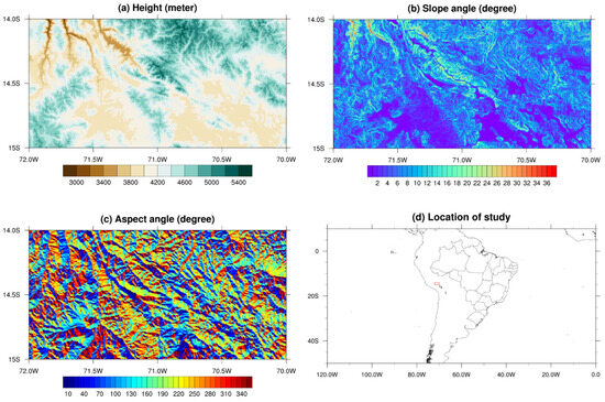
Figure 1.
Topographic data produced from the digital elevation model (DEM) of the Shuttle Radar Topography Mission, part of Andes Mountains (72° W:70° W, 15° S:14° S), (a) DEM (m), (b) slope height angle (degree), (c) slope aspect angle (degree), and (d) location of study indicated in red box.
4. Application to the Korean Integrated Model
The Korean Integrated Model (KIM) ([20]) developed by the Korea Institute of Atmospheric Prediction Systems is a global circulation model that uses a cubed sphere grid. This model has been used as the operating model of the Korea Meteorological Administration since April 2020. The operating version has a horizontal resolution of 12 km with 91 vertical layers up to 0.01 hPa. The regularly updated KIM uses a spectral element non-hydrostatic dynamical core and physics parameterization package. Therefore, the topographic data produced in a latitude–longitude grid with a 450 m resolution should be remapped in the cubed sphere grid of the KIM with a resolution of a few kilometers. We constructed a Voronoi tessellation for conservative area-weighted remapping from the latitude–longitude grid to the cubed sphere grid as described by [20]. One Voronoi cell is matched to each grid point of the cubed sphere, as shown in Figure 2. The horizontal resolution used in Figure 2 is about 830 km, which has been represented differently from the actual resolution to aid visual comprehension. The black points in Figure 2 are unique in the cubed sphere grid, where all dynamical and physical variables are computed. One Voronoi cell contains one unique point. For each unique point, we identified all high-resolution topographic data points (,) inside the Voronoi cell. Therefore, the average flux in Equation (4) is computed for N topographic high-resolution data points inside the Voronoi cell. For example, at a horizontal resolution of 12 km, one unique point at mid-latitude (40° N) had approximately 1600 topographic data points in the corresponding Voronoi cell. Using this method, all topographic data are matched to unique points of the cubed sphere grid without reuse of or missing topographic data. Coefficients A, B, and C are calculated at each unique point over the sub-grid N members identified from the Voronoi diagram. Figure 3 shows the A, B, and C coefficients of the Korean Peninsula in an 8 km resolution cubed sphere grid. (a) and (b) show the directional differences in the slope aspect angles (north–south or east–west) with the slope height angle, whereas (c) shows only height angle information. The Korean Peninsula is not a region where the topographic effects are as dramatically pronounced as the selected Andes Mountains in Figure 1. However, it is a significant target area for the KIM model to improve forecast performance. Therefore, the radiative topographic auxiliary data used for the Korean Peninsula is presented. The solar azimuth angle is also required to solve Equation (4). To obtain the solar azimuth angle, we require three formulas as a function of the declination and zenith angle of the sun and latitude and hour angle of the observers’ points (e.g., [21]). However, further and difficult circumstantial treatment is required to place the result from inversion of the trigonometric function into the correct quadrant.
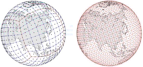
Figure 2.
(left) Cubed sphere grid of Korean Integrated Model (KIM) and (right) Voronoi tesselleation.
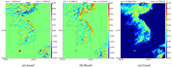
Figure 3.
A, B, and C coefficients of Korean peninsula in 8 km horizontal resolution of cubed sphere grid.
Ref. [7] proposed an alternative approach using the solar position and local direction, employing the Fortran intrinsic function atan2. Moreover, ref. [22] developed a concise formula for computing the solar azimuth angle based on the subsolar point and atan2 without circumstantial treatment. Using the formula suggested by [22], we computed the solar zenith and azimuth angles simultaneously, through a unit vector originating from the observer’s location and pointing toward the center of the sun. S gives unambiguous solution of the solar zenith angle and solar azimuth angle in the north–clockwise convention.
5. Results
The direct component of radiation in an ideal case with no absorption and no scattering at a horizontal resolution of 8 km was tested to validate the scheme. Figure 4 shows a snapshot of the flux difference experiment (EXP)-control (CTL) performed at 00 UTC on 21 June 2017. The Tibetan Plateau, with its vast expanse of high-altitude and complex terrain, has been extensively studied as a region for investigating the radiative topographic effects. Numerous prior studies have focused on this area ([13,15], etc.). Considering that the mid- and long-term performance of the East Asian region, including the Korean Peninsula, is directly influenced by the Tibetan Plateau, it is essential for the KIM model to accurately simulate the radiative input to the surface. The EXP contains a topographic radiative effect in the radiation module, whereas the CTL does not. The subsolar point at which the sun is perceived to be directly overhead is at approximately 173° E and 8° N in the middle of the Pacific Ocean. Depending on the relative position with respect to the sun, the illuminated and shadowed faces of the mountains are properly placed. The flux difference is particularly remarkable in rough terrain around the Tibetan Plateau. The cumulative global mean flux difference over 24 h (hourly calculation of the radiative process) is approximately 1.25%. However, this value is obtained in an ideal case of no absorption or scattering. In a realistic case with the same initial conditions, the 24 h cumulative global mean flux difference is almost zero.
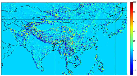
Figure 4.
Flux difference [experiment (EXP) − control (CTL)] of the incident direct radiation at surface assuming no absorption and scattering (Wm−2) in offline simulation. North is at top, South at the bottom, West to the left, and East to the right. One grid size corresponds to 4500 km.
After evaluating the offline ideal case, we performed a case study (8 km resolution) with the initial condition at 00 UTC of 6 July 2018. The atmospheric initial and surface boundary conditions are derived from the European Center for Medium-Range Weather Forecasts global reanalysis (ERA) version 5 (ERA5; [23]). The flux difference is less prominent than in the ideal case. We confirmed that the slope effect on the mountain faces was properly applied relative to the sun’s position. The most prominent feature is found near the Andes Mountains, as shown in Figure 5. In other regions, the radiative topographic effect was not prominent in the all-sky conditions between 18 and 24 h due to cloud perturbations. The averaged flux was extracted from the KIM’s standard output in 6 h intervals, which was averaged from 18 to 24 forecast times. The average solar zenith angle in this region during the corresponding output forecast time is approximately 60°. The flux level of EXP on the west side is larger than that on the CTL because the sun is on the west side of the map in the Pacific Ocean. In contrast, flux was smaller on the east side. The difference is more clearly observed in clear sky because the direct component of radiation drastically decreases in the presence of clouds. The flux difference varies from -30 to +30 Wm−2 depending on the slope position with respect to the sun. During the output frequency shown in Figure 5 (18–24 forecast times), the region is approximately maintained as clear sky such that the flux difference has a similar pattern in both clear and all-sky conditions. However, in other cloudy regions, the flux difference due to orography is erased by clouds because direct radiation is mostly scattered out before reaching surface. The cloud fluctuations begin to amplify right after the first radiation call, resulting in distinct cloud structures in a few hours that lead to the observed flux difference. The global mean flux difference in all skies was less than 0.01%.
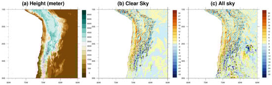
Figure 5.
Flux difference [experiment (EXP) − control (CTL)] of the incident radiation at surface. The map shows the Andes Mountain area (80° W:60° W, 35° S:15° S). The flux is time averaged from 18 to 24 forecast hours (6 h frequency output). (a). Height(meter); (b) Clear Sky; (c) All sky.
We ran a series of 10-day forecasts during one month of the boreal summer (1–31 July 2017) to examine the statistical performance. Both CTL and EXP have a horizontal resolution of 8 km and had 91 hybrid sigma-pressure vertical levels. Figure 6 shows geopotential height anomaly correlation coefficient (ACC) compared to ERA5. This ACC index was used as part of the standard verification package of KIAPS to test KIM for mid-term forecasting accuracy, and the details of this standard verification process are described in [24]. The comparison with ERA5 aims to evaluate the predictive performance of the model as the forecast time progresses. Although this scheme constitutes the largest impact among various factors of terrain-induced radiation effect, its influence decreases under all-sky conditions where the scattering radiation becomes dominant. This effect accumulates cumulatively towards the end of mid-term forecasts, manifesting in geopotential height, the most temperature-sensitive variable. Figure 6 indicates improvement in geopotential height across the majority of regions spanning the South Hemisphere, Northern Hemisphere, and the Tropical area. The East Asian region (60° E:144° E, 25.5° N:64.5° N), characterized by complex topology, particularly exhibits slightly superior improvement compared to other regions. Figure 7 shows the ACC and RMSE of geopotential height and temperature of the East Asian region. The ACC for this region at 850 hPa increased by 0.036 at 240 forecast hours. Other variables such as precipitation, humidity, and wind, excluding temperature and geopotential height, were found to be largely neutral between CTL and EXP. This scheme considers only the first-order effect of direct radiation influenced by the terrain, and quantifying the impact solely from the terrain effect under predominant cloud perturbations in all-sky conditions is challenging. However, it is expected that the radiative terrain effect will contribute to more accurate surface temperature predictions by simulating the time-varying solar energy input. Geopotential height, obtained by integrating temperature, provides a more sensitive assessment of model changes than temperature alone. In particular, the extensive Asia region highlighted in Figure 7, including areas with complex terrain, exhibited a more significant improvement in the geopotential height anomaly correlation coefficient compared to other regions, especially in the Northern Hemisphere. On the other hand, the global mean of the total radiative flux (both shortwave and longwave) is almost unchanged between CTL and EXP, as verified in the case study.
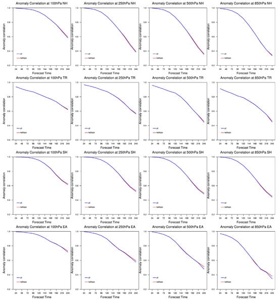
Figure 6.
Time series of the anomaly correlation coefficient (w.r.t ERA5) of geopotential height over (1st row) Northern Hemisphere, (2nd row) Tropical Region, (3rd row) Southern Hemisphere, and (4th row) East Asia.
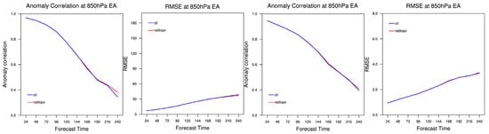
Figure 7.
Time series of the anomaly correlation coefficient and RMSE (w.r.t ERA5) of geopotential height and temperature over Asia (60° E:144° E, 25.5° N:64.5° N) at 850 hPa.
Additionally, we have depicted the temperature changes over the Korean Peninsula relative to Integrated Forecasting System (IFS) analysis data of the European Centre for Medium-Range Weather Forecast (ECMWF [25]) for a typical heatwave case on 6 July 2018, frequently employed for standard verification, in Figure 8. As evident in coefficient maps A, B, and C in Figure 3, the eastern side of the peninsula, adjacent to the sea, constitutes a region characterized by the representative mountain ranges of Korea, resulting in meteorological differences between the two regions centered around the mountain ranges. We observed a reduction in the extent of temperature anomalies during the summer heatwave event following clear-sky days.
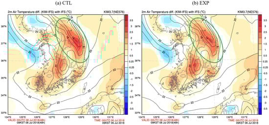
Figure 8.
Comparison of 2 m temperature (w.r.t. IFS) during the heatwave event on the Korean Peninsula at 48 forecast hours with an initial time of 00UTC on 6 July 2018. The most sloped area in South Korea is marked with a green oval line. (a). CTL; (b) EXP.
The greatest advantage of this scheme is its very low computational cost and memory requirements. Some coefficients must be calculated prior to the model run; however, this step must only be performed once for a given horizontal resolution, regardless of the initial condition or model starting time. Table 1 lists the average CPU time of the main radiation module during a 10-day forecast with a resolution of 24 km. Each run uses 9120 CPUs in a message passing interface environment. The main radiation module is called every hour, and each run has a total CPU time of 240 executions. Only a 0.58% increase in CPU time was observed for the 10-day forecast.

Table 1.
CPU computation time test for CTL and EXP. Each run uses 9120 CPUs in message-passing interface environments.
6. Discussion and Conclusions
We implemented subgrid-scale topographic effects on radiation using the global weather forecast model KIM, a model in which a typical grid size reaches at least a few kilometers. At this coarse scale of NWP, all topographic features are usually averaged and smoothed out. However, we developed a new scheme that considers subgrid-scale orography. The main characteristics considered in the scheme are the slope aspect, slope angle, and self-shading on the direct radiation solar flux. The slope factor is divided into time-dependent and time-independent parts. The time-independent part is a function of topographic data, and thus can be computed only once prior to all forecasting model runs. High-resolution topographic data were produced from the DEM of the Shuttle Radar Topography Mission on a regular latitude–longitude grid with a 15” horizontal resolution. The subgrid-scale data are linked to one grid of the KIM using a Voronoi diagram. Thus, all topographic high-resolution data are used without missing or reusing on the cubed sphere grid of NWP. The coefficients A, B, and C, defined in Equations (4) and (5), can be computed prior to the model run for a given resolution and are provided as ancillary data. This scheme was first verified using an ideal offline test. The observed flux difference (EXP-CTL) of the arriving direct solar radiation at the surface indicates that the scheme is properly applied. The flux difference varies from −30 to +30 Wm−2 depending on both the direction and altitude of the sun and slope. The scheme does not change the global mean energy balance, as shown in both the case and statistical tests. The statistical test of the mid-range forecast demonstrates improved temperature and geopotential height performance, particularly over land. The necessary ancillary file is only 95 MB in the case of an 8 km horizontal resolution of the KIM. The CPU requirement is almost negligible despite the additional calculation terms implemented in the new scheme.
The shadowing effects caused by surrounding sub-grid points have a significant impact especially when the solar altitude is low, but implementing such effects requires intensive computations and memory resources. As a compromise for application in operational global models, we have chosen to apply the scheme only when certain criteria are met. Currently, the criterion is based on the average slope value of the sub-grid points being lower than the solar altitude. However, as the number of sub-grid points involved in topography calculations within a grid point of the global-scale computation increases, the average slope value tends to decrease, potentially leading to less stringent criteria. In this study, the sub-grid topography data used had a horizontal resolution of approximately 460 m (15 s), while the horizontal resolution of the global-scale grid used in the experiments was about 8 km. In an ideal experiment that considered only direct radiation and excluded all scattering (gas, aerosol, clouds), the difference in cumulative flux was 1.25%. In real all-sky case, the percentage drops to 0.01%. Based on this result, we adopted this criterion for the 8 km horizontal resolution environment of the global-scale grid. In the future, as the resolution of the global-scale grid increases and the number of sub-grid points within a grid decreases, this criterion may become more suitable as a judgment criterion for applying radiation terrain effects. Ideally, introducing criteria that quantitatively and distinctly define the role of surrounding sub-grid points would be necessary.
Author Contributions
Conceptualization, S.B.; Methodology, S.B.; Software, S.B. and J.K.; Validation, S.B.; Formal analysis, S.B.; Data curation, S.B.; Writing—original draft, S.B.; Visualization, S.B. and J.K. All authors have read and agreed to the published version of the manuscript.
Funding
This work was conducted through the R&D project “Development of a Next-Generation Numerical Weather Prediction Model by the Korea Institute of Atmospheric Prediction Systems (KIAPS)”, funded by the Korea Meteorological Administration (KMA2020-02212).
Institutional Review Board Statement
Not applicable.
Informed Consent Statement
Not applicable.
Data Availability Statement
The ERA5 data can be obtained from the Climate Data Store (CDS; http://climate.copernicus.eu (accessed on 11 April 2024)). Software supporting this research is available in two technical reports of KIAPS, [3] and [13], not accessible to the public but it can be provided in a limited manner upon request to the author.
Conflicts of Interest
The authors declare no conflict of interest.
References
- Matzinger, N.; Andretta, M.; Van Gorsel, E.; Vogt, R.; Ohmura, A.; Rotach, M.W. Surface radiation budget in an Alpine valley. Q. J. R. Meteorol. Soc. 2003, 129, 877–895. [Google Scholar] [CrossRef]
- Oliphant, A.J.; Spronken-Smith, R.A.; Sturman, A.P.; Owens, I.F. Spatial variability of surface radiation fluxes in mountainous terrain. J. Appl. Meteorol. 2003, 42, 113–128. [Google Scholar] [CrossRef]
- Araghi, A.; Martinez, C.J.; Olesen, J. Evaluation of multiple gridded solar radiation data for crop modeling. Eur. J. Agron. 2022, 133, 126416. [Google Scholar] [CrossRef]
- Müller, D.M.; Scherer, D. A grid- and subgridscale radiation parameterization of topographic effects for mesoscale weather forecast models. Mon. Weather Rev. 2005, 133, 1431–1442. [Google Scholar] [CrossRef]
- Rontu, L.; Wastl, C.; Niemelä, S. Influence of the details of topography on weather forecast—Evaluation of HARMONIE experiments in the Sochi Olympics domain over the Caucasian Mountains. Front. Earth Sci. 2016, 4, 13. [Google Scholar] [CrossRef]
- Senkova, A.V.; Rontu, L.; Savijarvi, H. Parametrization of orographic effects on surface radiation in HIRLAM. Tellus A Dyn. Meteorol. Oceanogr. 2007, 59, 279–291. [Google Scholar] [CrossRef]
- Manners, J.; Vosper, S.B.; Roberts, N. Radiative transfer over resolved topographic features for high-resolution weather prediction. Q. J. R. Meteorol. Soc. 2012, 138, 720–733. [Google Scholar] [CrossRef]
- Arthur, R.S.; Lundquistm, K.A.; Mirocha, J.D.; Chow, F.K. Topographic Effects on Radiation in the WRF Model with the Immersed Boundary Method: Implementation, Validation, and Application to Complex Terrain. Mon. Weather Rev. 2018, 146, 3277–3292. [Google Scholar] [CrossRef]
- Gu, C.; Huang, A.; Wu, Y.; Yang, B.; Mu, X.; Zhang, X.; Cai, S. Effects of Subgrid Terrain Radiative Forcing on the Ability of RegCM4.1 in the Simulation of Summer Precipitation Over China. J. Geophys. Res.-Atmos. 2020, 125, e2019JD032215. [Google Scholar] [CrossRef]
- Lee, W.-L.; Liou, K.N.; Hall, A. Parameterization of solar fluxes over mountain surfaces for application to climate models. J. Geophys. Res. 2011, 116, D21111. [Google Scholar] [CrossRef]
- Gu, Y.; Liou, K.N.; Lee, W.-L.; Leung, L.R. Simulating 3-D radiative transfer effects over the Sierra Nevada Mountains using WRF. Atmos. Chem. Phys. 2012, 12, 9965–9976. [Google Scholar] [CrossRef]
- Liou, K.N.; Gu, Y.; Leung, L.R.; Lee, W.L.; Fovell, R.G. A WRF simulation of the impact of 3-D radiative transfer on surface hydrology over the Rocky Mountains and Sierra Nevada. Atmos. Chem. Phys. 2013, 13, 11709–11721. [Google Scholar] [CrossRef]
- Lee, W.-L.; Liou, K.N.; Wang, C.-C. Impact of 3-D topography on surface radiation budget over the Tibetan Plateau. Theor. Appl. Climatol. 2013, 113, 95–103. [Google Scholar] [CrossRef]
- Lee, W.-L.; Wang, Y.-C.; Shiu, C.-J.; Tsai, I.; Tu, C.-Y.; Lan, Y.-Y.; Chen, J.-P.; Pan, H.-L.; Hsu, H.-H. Taiwan Earth System Model Version 1: Description and evaluation of mean state. Geosci. Model Dev. 2020, 13, 3887–3904. [Google Scholar] [CrossRef]
- Hao, D.; Bisht, G.; Gu, Y.; Lee, W.L.; Liou, K.N.; Leung, L.R. A Parameterization of Sub-grid Topographical Effects on Solar Radiation in the E3SM Land Model (Version 1.0): Implementation and Evaluation over the Tibetan Plateau. Geosci. Model Dev. 2021, 14, 6273–6289. [Google Scholar] [CrossRef]
- Kondratyev, K.Y. Radiation Regime of Inclined Surfaces (WMO Technical Note 152, 82); World Meteorological Organization: Geneva, Switzerland, 1977. [Google Scholar]
- Farr, T.G.; Rosen, P.A.; Caro, E.; Crippen, R.; Duren, R.; Hensley, S.; Kobrick, M.; Paller, M.; Rodriguez, E.; Roth, L.; et al. The Shuttle Radar Topography Mission. Rev. Geophys. 2007, 45, RG2004. [Google Scholar] [CrossRef]
- Burrough, P.A. Monographs on soil and resource surveys. In Principles of Geographical Information Systems for Land Resources Assessment; Claredon Press: New York, NY, USA, 1986. [Google Scholar]
- Baek, S.; Kim, J. Producing Ancillary Files for Topographic Radiative Effects; Technical Report; Korea Institute Atmospheric Prediction System: Seoul, Republic of Korea, 2023; No. 2023-01. [Google Scholar]
- Hong, S.Y.; Kwon, Y.C.; Kim, T.H.; Esther Kim, J.E.; Choi, S.J.; Kwon, I.H.; Kim, J.; Lee, E.H.; Park, R.S.; Kim, D.I. The Korean Integrated Model (KIM) System for Global Weather Forecasting. Asia-Pacific J. Atmos. Sci 2018, 54 (Suppl. 1), 267–292. [Google Scholar] [CrossRef]
- Soulayman, S. Comments on solar azimuth angle. Renew. Energy 2018, 123, 294–300. [Google Scholar] [CrossRef]
- Zhang, T.; Stackhouse, P.W.; Macpherson, B.; Mikovitz, J.C. A solar azimuth formula that renders circumstantial treatment unnecessary without compromising mathematical rigor: Mathematical setup, application and extension of a formula based on the subsolar point and atan2 function. Renew. Energy 2021, 172, 1333–1340. [Google Scholar] [CrossRef]
- Hersbach, H.; Bell, B.; Berrisford, P.; Hirahara, S.; Horányi, A.; Muñoz-Sabater, J.; Nicolas, J.; Peubey, C.; Radu, R.; Schepers, D.; et al. The ERA5 global reanalysis. Q. J. R. Meteorol. Soc. 2020, 146, 1999–2049. [Google Scholar] [CrossRef]
- Lee, E.H.; Park, H.J.; Shin, H.J.; Lee, E.H.; Cho, G.H.; Cho, S.J.; Jung, J.Y.; Park, R.S. KIM Medium-Range Forecast Verification; Technical Report; Korea Institute of Atmospheric Prediction System: Seoul, Republic of Korea, 2021; No. 2021-01. [Google Scholar]
- Flemming, J.; Huijnen, V.; Arteta, J.; Bechtold, P.; Beljaars, A.; Blechschmidt, A.M.; Diamantakis, M.; Engelen, R.J.; Gaudel, A.; Inness, A.; et al. Tropospheric chemistry in the Integrated Forecasting System of ECMWF. Geosci. Model Dev. 2015, 8, 975–1003. [Google Scholar] [CrossRef]


Disclaimer/Publisher’s Note: The statements, opinions and data contained in all publications are solely those of the individual author(s) and contributor(s) and not of MDPI and/or the editor(s). MDPI and/or the editor(s) disclaim responsibility for any injury to people or property resulting from any ideas, methods, instructions or products referred to in the content. |
© 2024 by the authors. Licensee MDPI, Basel, Switzerland. This article is an open access article distributed under the terms and conditions of the Creative Commons Attribution (CC BY) license (https://creativecommons.org/licenses/by/4.0/).