Satellite Time-Series Analysis for Thermal Anomaly Detection in the Naples Urban Area, Italy

Abstract

Naples is the most densely populated Italian city (7744 inhabitants per km²). It is located in a particular geological context: the presence of Mt Vesuvius characterizes the eastern part, and the western part is characterized by the presence of the Phlegrean Fields, making Naples a high-geothermal-gradient region. This endogenous heat, combined with the anthropogenic heat due to intense urbanization, has defined Naples as an ideal location for Surface Urban Heat Island (SUHI) analysis. SUHI analysis was effectuated by acquiring the Land Surface Temperature (LST) over Naples municipality by processing Landsat 8 (L8) Thermal Infrared Sensor (TIRS) images in the 2013–2023 time series by employing Google Earth Engine (GEE). In GEE, two different approaches have been followed to analyze thermal images, starting from the Statistical Mono Window (SMW) algorithm, which computes the LST based on the brightness temperature (Tb), the emissivity value, and the atmospheric correction coefficients. The first one is used for the LST retrieval from daytime images; here, the emissivity component is derived using, firstly, the Normalized Difference Vegetation Index (NDVI) and then the Vegetation Cover Method (VCM), defining the Land Surface Emissivity (LSɛ), which considers solar radiation as the main source of energy. The second approach is used for the LST retrieval from nighttime images, where the emissivity is directly estimated from the Advance Spaceborne Thermal Emission Radiometer database (ASTER-GED), as, during nighttime without solar radiation, the main source of energy is the energy emitted by the Earth’s surface. From these two different algorithms, 123 usable daytime and nighttime LST images were downloaded from GEE and analyzed in Quantum GIS (QGIS). The results show that the SUHI is more concentrated in the eastern part, characterized by intense urbanization, as shown by the Corine Land Cover (CLC). At the same time, lower SUHI intensity is detected in the western part, defined by the Land Cover (LC) vegetated class. Also, in the analysis, we highlighted 40 spots (10 hotspots and 10 coldspots, both for daytime and nighttime collection) that present positive or negative temperature peaks for all the time series. Due to the huge amount of data, this work considered only the five representative spots that were most representative for SUHI analysis and determination of thermal anomalies in the urban environment.

1. Introduction

Global warming has been an ever-increasing phenomenon since the first industrial revolution, mainly due to human activity [1,2,3]. The IPCC Sixth Assessment Report (AR6) [1,4] confirms that the global surface temperature reached 1.1 °C above 1850–1900 values in 2011–2020. This temperature increase is due, principally, to human activities through emissions of greenhouse gasses. Global greenhouse gas emissions effects have continued to increase in the last decade, with an unequal historical and ongoing contribution arising from unsustainable energy use, land use, and land-use changes in lifestyles and patterns of consumption and production across regions [4]. Human-caused climate change is already affecting many weather and climate extremes across the entire globe. Evidence of observed changes in extremes such as heatwaves, heavy precipitation, droughts, and tropical cyclones has also been strengthened in the IPCC Assessment reports [5,6], which highlight that hot extremes (including heatwaves) have become more frequent and more intense since the 1950s, as the global population has increased. A heatwave may be defined as a period where local excess heat accumulates over a sequence of unusually hot days and nights [3]. Heatwaves in urban environments are often exacerbated by the “Surface Urban Heat Island” (SUHI) effect [7], meaning that the increase in temperature within the urban environment is greater than in surrounding rural areas due to human activities, altered land surfaces, and increased energy consumption [7]. Over the past 20 years, SUHI has been an increasing phenomenon in several Italian cities; more precisely, in summer 2023, different Italian regions recorded temperature records due to the strong heatwave in July 2023 and the relative SUHI that was generated in several cities. Examples of these elevated temperatures are 46.3 °C in Cagliari, 39 °C in Naples, and 42.9 °C in Rome, reached on 18 July [8]. Northern Italy also recorded maximum temperature values in July 2023, like in Turin and Milan, with temperatures above 40 °C. During these heatwaves, temperatures remained extreme even at night, with values above 30 °C; these are temperature values far above seasonal averages, posing serious health risks to the elderly, children, and those most at risk [9,10,11]. The SUHI phenomenon has been known since the 19th century, with the exponential growth of urbanization, but has only recently attracted scientific interest. In Italy, Naples is a representative city that is characterized by the higher urbanization rate, and the SUHI issue is compounded by dense construction, limited green spaces, and a growing population. As a result, the city faces elevated temperatures, which can have adverse effects on public health, energy consumption, and overall quality of life. Therefore, we focus this paper on Naples, which offers a suitable geographical context and long-term data availability to approach this issue. Despite the high volcanic risk due to the presence of active volcanoes such as Vesuvius and Phlegrean Fields, Naples is one of the most densely urbanized areas and has about 1.5 million inhabitants, making it the most densely populated Italian city. Due to urban development, the city is affected by a pronounced heat island, accentuated by the density of building areas, narrow streets, small parks, and a particularly tight architecture that limits air circulation, adding to a high geothermal gradient due to volcanic activity [12]. Within an urban area, the temperature is not recorded uniformly but rather is a function of the percentage of vegetation present and land use. It is a common experience that an urban area has higher temperature values than the surrounding rural or non-urbanized areas [7,9,13]. This temperature difference depicts one or more smaller urban sectors that can be affected by SUHI, which is attributed to the change in energy exchange between urban heat surfaces and the atmosphere, primarily caused by increased surface cover replacing cooler vegetation surfaces and anthropogenic heat releases [14]. Different strategies have been analyzed to reduce the SUHI effects; according to one set of authors, heat island mitigations can be performed by increasing the presence of parks and plants [15], i.e., vegetation that can absorb light radiation because of the high albedo, generating a cooling effect and taking advantage of evapotranspiration [16]. On the other hand, sustainable materials for construction and asphalt (cool and green roofs, reflecting asphalt) are being studied to reduce the materials’ ability to absorb heat [17,18,19,20,21].

1.1. Aim of the Work

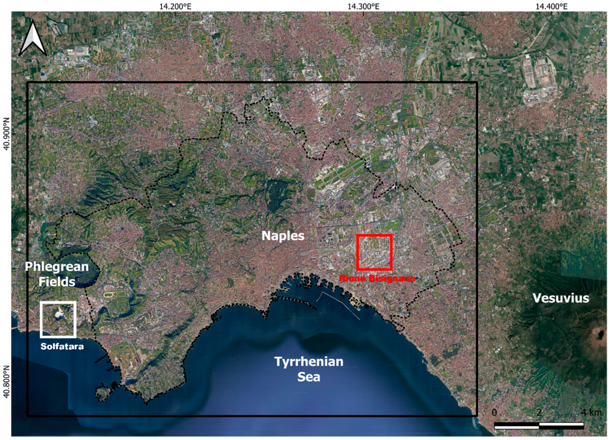
The purpose of this work is to define/detect the SUHI on the Naples urban area by analyzing the variation in both the time and spatial domains of the surface temperature over land. This analysis has been performed by using multispectral remote-sensed data that are suitable to retrieve the Land Surface Temperature (LST) and are available for the last 10 years; the United States Geological Survey (USGS) Landsat catalog has been used. To process this huge amount of data, GEE procedures [22] have been used to define the maximum intensity of SUHI found close to Garibaldi Square near the Central Station (Naples); high temperatures in this area may be attributed to the high urbanization and also to the presence of a high concentration of low-albedo materials, such as asphalt pavements or dark roofs, with absence of vegetation favoring the absorption of solar radiation [23]. From the Google Earth Engine (GEE), 59 daytime and 64 nighttime images, from 2013 to 2023, for a total of 123 images, were downloaded and analyzed by using QGIS (release 3.28), computing both spatial and temporal analyses. In the GIS environment, the isotherms were clusterized, with a temperature range of 3° to identify pixels that were characterized by excessive (hot and/or cold) temperature values for both daytime and nighttime collections. Pixels with lower temperature values were defined as coldspots (CS), while the ones that represented higher temperature values were the hotspots (HS). From the spatial analysis, 40 spots (10 hotspots and 10 coldspots for each daytime and nighttime collections) were identified within Naples’ territory. To better comprehend the correspondence between the spot location and land use, an overlap of the Corine Land Cover (CLC) [24] was effectuated. The temporal analysis results showed that, for the entire time series, the urban class is the best guess for the hotspots, while the vegetated class hosts the coldspots. Two anomalies are highlighted: one refers to the pixel located on the Solfatara vent located in the western part of the study area, and the second one refers to the locomotive depots located in the eastern part of the study area in Rione Bisignano (Figure 1).

1.2. Study Area

This study is focused on the Naples urban area, located on the west coast of southern Italy. Naples is the most densely populated city in Italy, with about 1.5 million inhabitants in an area of 117 km², making it the most densely populated city nationally, with 7744 inhabitants per square kilometer [25]. Naples is situated close to two main volcanic areas: the Phlegrean Fields (located in the western part in proximity to Pozzuoli municipality) and Mt. Vesuvius (located in the eastern part) (Figure 1). The geomorphology of this region is strictly dependent on structural highs generated by these two nested calderas, creating several steep scarps and cliffs that may affect the incoming solar radiation and generate important temperature variations. Nowadays, Phlegrean Fields are defined by bradyseism and degassing activity, especially in the Solfatara region, where the temperature, at the vent may reach maximum values of 147 °C [26,27,28]. The urban center is in the southern part of the city (in proximity to the coast), while the industrial area is concentrated in the east-northeastern part and the northern part of the city. In contrast, the western part, where Phlegrean Fields craters are present, is less urbanized and, therefore, is more vegetated due to the impossibility of building in a geologically active area. Naples presents a Mediterranean and humid subtropical climate, characterized by hot, dry summers and cool, wet winters [29]. Precipitation is concentrated principally in the spring and fall seasons and is about 1006.6 mm/y. The mean annual temperature is 15.5 °C. Summer is characterized by average daily temperature ranges from 17.2 °C to 28.3 °C, while, during winter, temperature ranges from 4.4 °C to 13.1 °C [30]. Because of the climatic conditions and urban development, during summers, when temperatures are elevated and precipitation is minimal, the city is affected by a pronounced heat island, accentuated by the distribution of building areas, narrow streets, small parks, and a particularly tight architecture that limits air circulation [19]. The Neapolitan area is affected by three main heat contribution effects: anthropogenic heat sources due to intense urbanization, endogenous source heat due to dominant volcanic activity (at a very local scale, i.e., near Phlegrean Fields), and the surrounding sea which operates as a mitigator, close to the sea (coastal area near the shoreside) [31]. Considering the conditions mentioned above (population density, urban texture, and heat sources), Naples represents a suitable area to test the solution proposed in the definition of SUHI.

2. Materials and Methods

To perform the SUHI estimation, an approach based on the assimilation of remote-sensed data, used for both the definition of brightness temperature and emissivity values and the parametrization of the atmosphere (to define its effects on the LST estimation), has been used. The satellite data were obtained from the Landsat Thermal Infrared Sensor (TIRS) and the Advanced Spaceborne Thermal Emission Radiometer (ASTER) sensors. The atmospheric parameters were provided by the National Center for Atmospheric Research (NCAR) and the National Center for Environmental Prediction (NCEP). In the next paragraphs, input and procedure are better described.

2.1. Data

2.1.1. Satellite Data LST

Since 1972, Landsat satellites have consistently gathered imagery of the Earth’s surface, building an unparalleled historical archive. The extensive collection, housed in the USGS archives, serves as a valuable scientific resource for users across the globe. Landsat 8 (L8), launched on 11 February 2013, which, at the start of the time series, stands as the most recent satellite in the series [32,33], incorporates two primary sensors: the Operational Land Imager (OLI) and the TIRS. OLI captures images through nine spectral bands in various wavelengths of visible, near-infrared, and shortwave electromagnetic energy. This allows for the observation of a 185 km wide swath of the Earth, with a spatial resolution ranging from 15 to 30 m. This spatial resolution is sufficient to discern features such as urban centers, farms, forests, and other land uses, covering extensive areas of the Earth’s landscape. On the other hand, TIRS images include two bands (10 and 11) that contribute to more precise surface temperature measurements and are collected with 100 m spatial resolution. For easier use by users, the USGS made a resampling with cubic convolution; hence, bands 10 and 11 have 30 m resolution in the delivery product data, coinciding with the OLI and TIRS spatial resolutions. The approximate scene size is 170 km north–south by 183 km east–west. To compute the surface temperature using L8 data, despite its two thermal bands, it is noteworthy that, in considering the caution issued by the USGS regarding the utilization of Band 11 due to calibration uncertainties [34], the application of the single-channel algorithm has been directed towards Band 10.

2.1.2. Emissivity

Emissivity is an intrinsic property of a material, is often regarded as an indicator of material composition, and can be derived from the emitted radiance measured from space [35]. Emissivity is a dimensional quantity that can range between 0 and 1; the two extreme values refer to a body that reflects the full incident radiation (ɛ = 0) and to a body that absorbs the full incident radiation (ɛ = 1), respectively. Between these two values, each different material assumes a different emissivity value (e.g., Sand = 0.9, Snow = 0.8, Soil (Dry) = 0.92, Soil (Saturated) = 0.95, Water = 0.95, Solar panels = 0.94) [35,36]. Considering the role of surface emissivity in surface temperature retrieval, the ASTER Global Emissivity Dataset (GED) emissivity data, available for free download on the USGS website [37], were used. The ASTER-GED land surface temperature and emissivity data products are generated using all clear-sky pixels of ASTER scenes acquired from 2000 through 2008, with a spatial resolution of 100 m [38]. In this study, considering that L8 data are delivered at 30 m but acquired at 100 m, the ASTER-GED emissivity is appropriately resized to match the L8 pixel spatial resolution. To tighten the historical series, we decided to also add the L8 daytime passages, doubling the amount of data.

Whilst the ASTER-GED data set is used to process nighttime images, to process the daytime L8 acquired images, we decided to use the emissivity value estimated by the relation between Normalized Difference Vegetation Index (NDVI), Fractional Vegetation Cover (FVC), and emissivity. The association between the emissivity value and the percentage of vegetation cover is explained by the NDVI, which uses spectral reflectance ($\rho$) in the near-infrared (NIR) band and the red (R) band (L8, OLI, band 4 and band 5); it is defined as

$$NDVI=\frac{\rho NIR-\rho RED}{\rho NIR+\rho RED}$$

(1)

NDVI values range between −1 and 1; higher NDVI values indicate high vegetation vigor, while lower NDVI values indicate low vegetation cover (typically from 0 to 0.2), like water bodies or bare soil [37,39].

In this paper, NDVI threshold values are useful to define the FVC, an index that estimates the proportion of an area covered by vegetation and, consequently, the fraction of green vegetation viewed by the sensor [29,31]:

$$FVC=(\frac{NDVI-NDVIb}{NDVIv-NDVIb}){ }^2$$

(2)

where NDVIb and NDVIv are NDVI threshold values for bare soil pixels and vegetation soil pixels, respectively [17]. Under global conditions, values of NDVIv = 0.86 and NDVIb = 0.2 have been proposed by [22,40,41]. According to the Vegetation-Cover Method (VCM), based on the assumption that the effective emissivity of a given area can be modeled as a linear combination of the emissivity of the vegetated and bare ground portions of an area, it is possible to define the land surface emissivity (LSɛ) as

$$LS\epsilon =FVC\epsilon veg+(1-FVC)\epsilon bare$$

(3)

where ɛveg and ɛbare are the values computed for vegetated soil and bare soil, respectively. The emissivity of vegetated surfaces shows low variation in the TIR region; hence, this value is prescribed as constant and equal to ɛveg = 0.99 [22]. LSɛ is an intrinsic property of all materials that measure their efficiency in converting heat into radiation; it represents a critical variable in the quantification of the surface energy budget and for the estimation of surface parameters from earth observation data [41,42]. LSɛ values extracted by the VCM method are strictly dependent on the surface classification and may not represent variability associated with changes in surface conditions. Indeed, the assigned emissivity value for a particular pixel may be inaccurate if it does not fully represent the complexity of the surface [43]. LSɛ retrieval through the VCM here is used for the LST computation in the daytime image collection, where it is possible to exploit the Reflectance of Solar Radiation by vegetation to calculate NDVI and FVC because of the correlation between the emissivity value and the vegetation cover of the surface. However, for the nighttime image collection, when solar radiation is absent and the main source of energy is emission by the Earth, it is preferable to use a global database of emissivity values such as ASTER-GED to cope with the difficulty in estimating emissivity in the absence of solar radiation.

2.1.3. Atmospheric Correction Coefficients (A, B, and C)

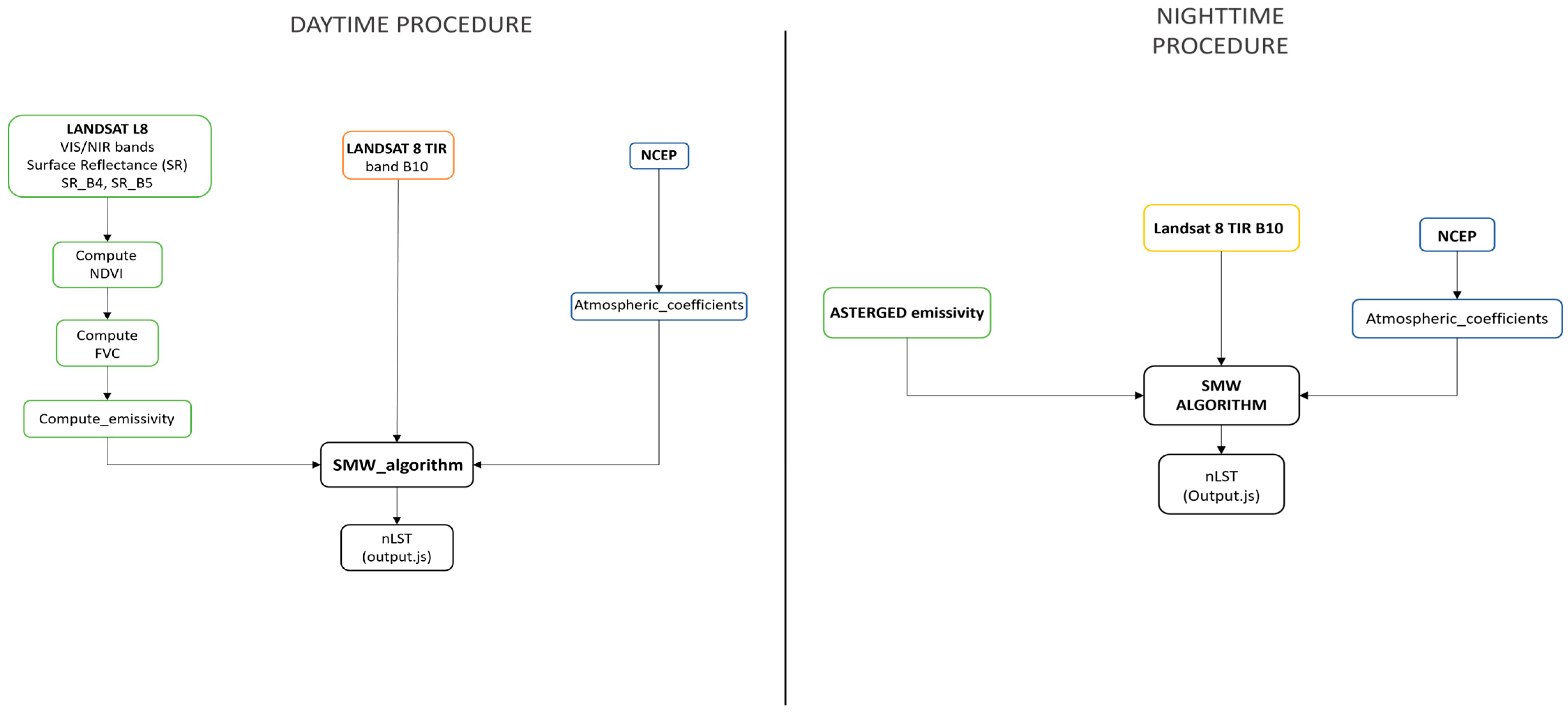
Information on the atmospheric water vapor content is required to better account for atmospheric contributions in the TIR observations [22]. Correcting for the atmospheric effects requires accurate knowledge of the vertical profiles of atmospheric water vapor and temperature, both of which are highly variable. The information about the Total Column Water Vapor (TCWV) values is provided by the NCAR and NCEP and are all available on GEE with the NCEP/NCAR reanalysis collection [15]. From the NCEP/NCAR collection, atmospheric water vapor data are extracted to define the Total Precipitable Water (TPW), which is a product that represents the total integrated moisture in the atmospheric column from the surface to the Top of Atmosphere (TOA). Therefore, for every daily and temporal interval, a precise value of TPW has been assigned on a scale of 10 classes (from 0 to 9), with an interval of 6 cm in the water vapor column.

2.2. Processing

The SUHI estimation is based on the Statistical Mono Window (SMW) algorithm, proposed by [22]. This algorithm is dedicated to processing single-diurnal images and estimating the LST. We have modified this procedure to process time series for both daytime and nighttime images due to differences in the emissivity estimation. The original SMW performed to estimate the LST is defined as follows:

$$LST=A\frac{Tb}{\epsilon }+\frac{B}{\epsilon }+C$$

(4)

where the variables are as follows:

Tb = Brightness temperature, which is derived from L8 TIRS data by using the thermal channel centered at 11 μm, which corresponds to band 10;

ɛ = emissivity. Emissivity values are necessary for LST computation from Tb images;

A, B, C = atmospheric correction coefficients. These are required to constrain the atmospheric contributions in the TIR observations [22].

The paradigm adopted in this study relies on the GEE platform to process the L8 archived dataset, which is composed of an unpredictable number of images. The GEE platform employs web access based on JavaScript language and Python, which makes it extremely versatile to elaborate data without downloading data onto local premises. It also takes advantage of re-use scripts already developed by other users such as the code proposed in [22] (

Table 1. Satellite, bands, GEE dataset, and ETC for the daytime collection.

Satellite	Bands	Wavelength (μm)	GEE Dataset	Equatorial Crossing Time
Landsat 8 (OLI, TIRS)	RED B4	0.64–0.67	LANDSAT/LC08/C02/T1-L2	10:00 a.m. 16 days
	NIR B5	0.85–0.88	LANDSAT/LC08/C02/T1-L2
	TIR B10	10.06–11.19	LANDSAT/LC08/C02/T1_TOA

). Following this approach, the procedure in [22] has been modified to process the L8 2013–2023 daytime and nighttime time series, obtaining an estimation of the LST over Naples.

Since, in previous work [15], the SMW algorithm in GEE is applied only for a single daytime image, to increase the density of the analyzed collection, it was necessary to readapt the code in [22] for the LST retrieval in the nighttime by adopting ASTER-GED emissivity. When the main energy source is the Sun’s radiation (during daytime), the surface emissivity is computed by starting from the FVC retrieval and the VCM method due to the correlation between the emissivity value and the vegetation cover on the surface [44]. To obtain the FVC, in [22], the NDVI was computed from the Surface Reflectance L8 collection band 4 and band 5. Finally, following Equation (3), LSɛ is obtained for the daytime collection. Without the Sun component (during nighttime), the main source of energy is not the solar radiation reflected by the Earth to the sensor, but is the energy emitted by the Earth itself; thus, it is not possible to use methods that are reflectance-based. In ASTER-GED, the TIR emissivity is defined by ASTER band 13 because of its similarity to the Landsat 8 band 10 wavelength (

Table 2. Satellite, bands, GEE dataset, and ETC for the nighttime collection.

Satellite	Bands	Wavelength (μm)	GEE Dataset	Equatorial Crossing Time
Landsat 8 (OLI, TIRS)	TIR B10	10.06–11.19	LANDSAT/LC08/C02/T1_TOA	10:00 a.m. 16 days
Terra (ASTER)	TIR B13	10.95–10.95	NASA/ASTER_GED/AG100_003

).

The use of nighttime data allows us to avoid both direct solar heating and the topographic effect, minimizing their influence, as well as rendering the reflectance component negligible. Another advantage of nighttime images is that surface temperature is more constant than in daytime due to the absence of solar radiation, and temperature values are dependent only on the thermal energy remitted by buildings [45]. The TOA brightness temperature is provided by L8 band 10, queried through the GEE capabilities, and is common for daytime and nighttime procedures. The emissivity is obtained using different methods that depend on the acquisition timing. The LST retrieval tailored code requires the same input data for the atmospheric correction, obtaining a flexible version of the SMW algorithm (Figure 2).

As seen in Figure 2, both daytime and nighttime codes present several different subroutines. These codes are started by the main subroutine, which is the Landsat_LST, which includes the L8 TOA collection and the L8 SR collection (this collection is applied only for the daytime LST retrieval). L8 SR is used for extracting the VIS (red) and NIR bands (SR_B4 and SR_B5) that are applicable for the NDVI computation; meanwhile, the TOA_B10 is directly imported into the final LST retrieval. In the daytime code, the following subroutines refer to the emissivity definition, starting with NDVI (compute_NDVI), FVC (compute_FVC), and the final subroutine (compute_emissivity) in which the NDVI and FVC subroutines are required, and the surface emissivity is calculated starting from Equation (3). These steps, which are useful for the emissivity computation in the nighttime code, are not required because the emissivity is directly extrapolated by band 13 of the ASTER-GED dataset. In both codes, in addition to the operations described above, there is the atmospheric correction retrieval, which comprehends the NCEP_TPW subroutine, where the atmospheric water vapor data are matched to each Landsat image. Then, in the SMW_coefficients subroutine, all the atmospheric coefficients are computed. Finally, all the components for the LST retrieval are defined and required in the final subroutine, which is the SMW_algorithm. Within that, based on Equation (4), the A, B, and C coefficients, defined in the SMW_coefficient subroutine, are applied and the emissivity is computed by the FVC method or by ASTER-GED and the Tb extracted by the TOA B10. In the Output subroutine, the LST retrieval for the daytime and nighttime images is shown and, in the task window, it is possible to download the LST images. The Output subroutine also presents the string for the batch download, which permits one to download the entire LST image collection. In QIS, from the images, isotherms were extracted with a range of 3 degrees to identify those pixels characterized by extreme temperature for both nighttime and daytime collections. Based on the average temperature values in the images, the authors decided on the scale of 3 degrees to represent the temperature scale that was used to individuate the spots.

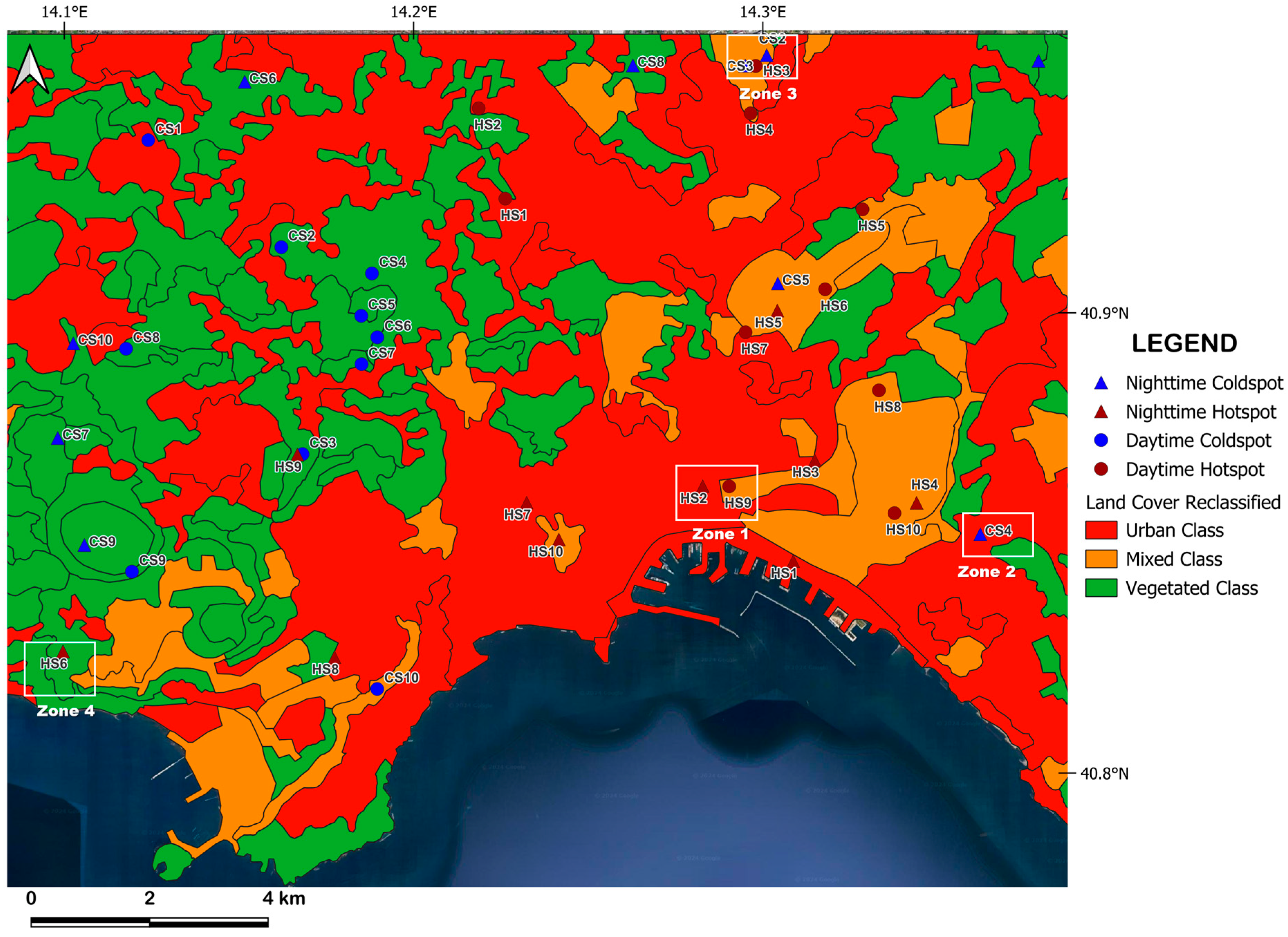
2.3. Results Characterization by Using the Land Cover

To better comprehend the characterization of urban thermal environments, including the SUHI effect, the authors investigated the relationship between LST and Naples’ land cover and soil use using the Corine Land Cover (CLC). CLC is the database of Copernicus Land-Monitoring Service (CLMS) and represents the European reference for land-cover and land-use inventory [46]. The CLC includes land-use/land-cover (LULC) status for European countries [47] and represents the spatial distribution of different types of physical coverage of the Earth’s surface. For the sake of this work, the 44 standard thematic classes (CLC-2018) have been newly clusterized to match the L8 Ground Sample Distance (GSD) of the remote-sensed data used (90 × 90 m). Indeed, for this paper, considering the complexity of the study area and the granularity of the information in the CLC classification, CLC may be overly detailed, and no significant differences in temperature between similar classes are noticed. For this reason, and considering the L8 GSD, it was decided to simplify the land-cover classification by reducing it into three main macro-classes: the first class refers to the urban area, the second refers to the vegetated area, and the third one refers to mixed area, i.e., sparse vegetation and discontinuous urbanization (Figure 3).

3. Results and Discussion

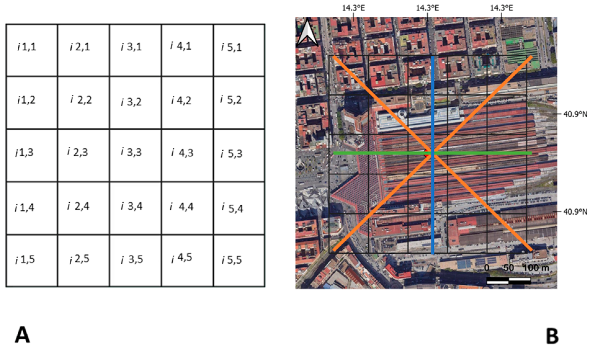
In this section, the results are shown. A total of 434 daytime images and 230 nighttime images were downloaded from the task window in GEE, according to the methodology previously illustrated. For the sake of the quality of results, cloudy images were removed and not processed. For the daytime collection, the code provided by [22] presents a cloud-mask sub-routine, but, for nighttime images, due to the complexity of the atmospheric parameters’ definition, it is not reasonable to use a cloud mask; hence, to apply the same analysis method to both daytime and nighttime collections, cloudy images have been removed manually. After this removal phase, 123 images constitute the bulk of the images to be processed for the SUHI analysis—64 nighttime and 59 daytime. Images in both collections present a half-pixel shift, for this reason, to build a unique stack, with the images coming from different platforms. QGIS software version 3.28 has been used to pile up the 123 used images by utilizing the “co-registration” plug-in, where it considered a reference nighttime and daytime image to construct the co-registered stack.

Spatial Analysis

Spatially analyzing the studied area, in a general view, two main clusters can be identified (Figure 3): a warmer eastern zone, which can be attributed to the urban center and industrial area of Naples, and a cooler western zone, near the Phlegrean Fields craters and the vegetated area to the north. This spatial pattern is coherent with [29], which shows that the spatial disposition of hotter areas and cooler areas is also strictly dependent on NDVI values. In the entire time series, there are individual pixels that constantly show the highest or the lowest temperature values. Pixels that show the highest temperature values are named hotspots and pixels characterized by the lowest temperature values are named coldspots, with a total number of 40 spots (10 daytime hotspots, 10 daytime coldspots, 10 nighttime hotspots, and 10 nighttime coldspots). These spots represent the positive or negative extreme temperature compared to the images’ mean temperature. Temperature trends around each spot are inspected by building a 5 × 5 pixel grid, where the cell i_3,3 (Figure 4A) corresponds to the spot and the other 24 cells are the background. It is important to highlight that cells are ordered following a column per row disposition. Within each grid, the mean temperature of each cell (which corresponds to the pixel mean temperature) is extracted by univariate statistics, computed in GRASS GIS with the v.rast.stat plugin. In the grids, we have defined four different directions along the temperature values that were studied to comprehend the behavior around the spot. Two directions represent the 1,1–5,5 and 1,5–5,1 diagonals, while the third one is E–W (i.e., from 1,3 to 5,3 in the matrix cells) and the fourth one is N–S (from 3,1 to 3,5) (Figure 4B).

From the univariate statistic, it was revealed that temperature behavior is coherent, with CLC showing that the urban class is characterized by higher temperature values and that vegetated class is characterized by the lower. This affirmation is also confirmed by the NDVI: pixels with lower NDVI values, related to sparse vegetation, as is typical of urban areas, present higher temperature values, while vegetated pixels characterized by higher NDVI values show lower temperature. More precisely, hotspots, both diurnal and nocturnal, are concentrated more in the eastern part of the city of Naples, characterized by the urban center and industrial area. In contrast, coldspots are concentrated more in the western and northern portions of the study area, which are characterized by the vegetated class of CLC. In addition, five spots were identified that could be grouped into four different zones (Figure 3) that show singular temperature behaviors and are explained individually.

The results of the statistics for each of the four directions within the grid are represented as four different graphs, where the Y axis represents the temperature and the X axis is the cell i_xy. Within each graph, we report the temperature profiles for each date of the time series for all the directions (Figure 5, Figure 6, Figure 7, Figure 8 and Figure 9).

The first zone (Zone 1, Figure 3) is Garibaldi Square, in the city center (Figure 5a), and it is characterized by the presence of the Naples Central Station. At the “grid” scale in the area, there is no vegetation—the square is surrounded by tall buildings and narrow streets. Within this area, we observe both Nighttime HS2, slightly west of Garibaldi Square, and Daytime HS9, located close to (and to the north of) the Central Station. Nighttime HS2 shows no notable changes in temperature over the historical series, but the particularity of Nighttime HS2 is that, despite being nocturnal, it shows some of the highest temperature values achieved within the urban CLC class and over the entire time series. On summer nights, the temperature at pixel i_3,3 exceeds 40 °C (Figure 5b–e).

Daytime HS9 includes the rooftop of Naples Central Station (Figure 6a). Throughout the area, no vegetation is present and long iron structures cover the tracks. The temperature, as seen in the graphs (Figure 6b–e), is higher in all the pixels that fall above the tracks that run in the W–E direction, while the lower temperature values fall instead in the pixels that cover the building outside the station in the northern part of the analyzed grid (indices from i_1,1 to i_5,1). During daytime, the higher temperatures are above the iron structures due to the high thermal conductivity of the iron materials and because of the elevated emissivity value (i.e., 0.7–0.95 in the 8–14 μm wavelength range), increasing the indoor ambient temperature, resulting in the use of air conditioners to cool indoor air but contributing to a greater increase in outdoor temperature. Considering the vicinity of the hottest pixels for both the Nighttime HS2 and Daytime HS9, we can assume that this can be defined as the hottest zone within the study area.

The second zone where we focus our attention is Zone 2 (Figure 3). It hosts the unique nighttime coldspot that falls within the CLC urban class, named Nighttime CS4, and it is coincident with the roof of the Ente Autonomo Volturno (EAV) locomotive depot (Figure 7a). By analyzing the obtained results (Figure 7b–e), despite the complexity of the figure, we emphasize that the temperature has a constant value until 2018; after this year, the i_3,3 is characterized by a temperature decrease of about 7 °C, also confirmed by a negative value of the linear regression of cell i_3,3. By a qualitative visual inspection through a comparison with the historical images on Google Earth, after 2018, a solar panel was installed above the roof of the analyzed depot. After this installation, a significant reduction in the temperature of the area during nighttime was recorded. Indeed, from the graphs in Figure 7b–e, the trend of the curves is evident, with a point of inflection after 2018. Our interpretation of this temperature decrease is to relate to the solar panel installation. During the day, the Sun’s rays strike the outer surfaces of the solar panel, which is glazed, and are absorbed by a black capturing plate that heats up. During the night, these materials do not absorb energy but rather cool very quickly, recording a temperature decrease that is directly connected to the signal inversion due to the failure to absorb energy.

A similar case is described by the Nighttime CS2, located at the northern boundary of the investigated area (Zone 3, Figure 3). This coldspot includes the roof of the SEDA SpA packaging factory (Figure 8a), which belongs to the mixed urban/vegetation class of CLC (Figure 3). In this area, the temperature was quite constant until 2021; from the images, in January 2022, there is an important decrease in temperature, with the absolute minimum of the time series touching −9.99 °C (i_3,3) just above the structure (Figure 8b–e). As for the previous coldspot, Nighttime CS2 shows a negative value of linear regression, and, from a qualitative visual inspection through a comparison with the historical images on Google Earth, it is evident that, in September 2021, the roof of the structure was probably coated with reflective paint. Reflective paints are high-emissivity paints that can reflect the Sun’s rays while keeping the surfaces they cover cool. The use of reflective paints accompanied by several different techniques, such as cool roofs, green roofs or, indirectly, the installation of solar panels, represents the main SUHI mitigation effort [48,49].

The last area (Zone 4, Figure 3) that the authors decided to highlight is the Nighttime HS6, which includes the Solfatara crater, one of the active craters of the Phlegrean Fields (Figure 9a). The Phlegrean Fields is a multi-center volcanic complex with two nested calderas, Campanian Ignimbrite (39 ky) and Neapolitan Yellow Tuff (14 ky), situated northwest of Vesuvius. It is a volcanic belt composed of dozens of eruptive, explosive, and effusive centers over an area of more than 200 km². After the last eruption of Monte Nuovo occurred in 1538, the volcanic complex was characterized by quiescence [28]. Minimal volcanic activity is recorded only by the bradyseism phenomena and through fumarole emission, i.e., Pisciarelli and the Solfatara, both characterized by an intense SO₂ degassing, also monitored by the ground station placed near the vent [26]. More precisely, the Nighttime HS6 is located above the Solfatara and consists of the unique hotspot located in the vegetated CLC class. As shown in the graphs (Figure 9b–e), the temperature trend is constant through the time series, with the temperature peaks reached right near the vent. Lower temperature values occur where vegetation is present and volcanic activity is not present. It is important to note that this spot is recognized as a hotspot only by nighttime images whilst, during the day, there is no evidence of such behavior. The Solfatara is in an area where the temperatures are normally lower than the surrounding urban area; hence, during the day, this spot cannot be detected as a hotspot because of the higher urban center temperature. The Solfatara is characterized by a higher geothermal gradient: it can only be detected during the night, when temperatures in the urban area decrease because of the absence of sunlight, while, in volcanic areas, due to the elevated geothermal gradient, the surface temperature also remains constantly high during the nighttime.

4. Conclusions

In this paper, the LST retrieval over the Neapolitan area has been effected by processing data from the high-resolution L8 TIRS sensor. The algorithm proposed for the LST retrieval is the SMW, which requires, as input, the brightness temperature, the surface emissivity, and the atmospheric coefficient (NCEP collection). The surface emissivity has been derived with two different procedures, according to the timing of the Earth Observation (EO) data used: estimated by the NDVI for daytime and from the ASTER-GED collection for the nighttime images. By applying the SMW algorithm, 123 images, both diurnal and nocturnal, were obtained, and they were statistically examined using QGIS release 3.28. In total, 10 hotspots and 10 coldspots for both nighttime and daytime have been highlighted, and 4 zones show particular temperature trends. The statistical temperature analysis computed by QGIS has shown a hot region surrounding Naples’ urban center; in particular, the hottest area is in Garibaldi Square, and the coolest area is close to the Phlegrean Fields in the western sector. It is important to underline that the Nighttime HS6 (Solfatara crater) is the only hotspot located in the vegetated area. This hotspot is detected only in nighttime images. This means that, during daytime, the LST retrieved for this area is not significant for the surrounding zone. On the contrary, nighttime data are suitable to detect the natural thermal source represented by the Solfatara di Pozzuoli; therefore, this method can also be suitable for monitoring purposes.

The use of mitigation measures (e.g., cool roofs) produces a positive effect on the SUHI intensity; furthermore, vegetation can be considered to reduce the variation of the surface temperature and for mitigating high temperature, which is becoming a health issue. Solar panel installation (e.g., at Nighttime CS4) is not considered a proper mitigation measure. Still, nocturnal remote-sensed data show a signal inversion—recorded as a decrease in temperature—because of the absence of irradiation of the solar panels by solar radiation.

This work, merging innovative solutions (GEE) and using consolidated algorithms and procedures for remote-sensed data analysis, shows a versatile procedure for the SUHI definition and monitoring. The paradigm used can be exported to any geographical area to also allow a historical analysis, considering that the Landsat mission, with the updated version, has been orbiting since 1972. At the same time, remotely sensed data used in the UHI monitoring may present some limitations, like the necessity to use cloud-free images, which greatly decreases the number of usable images within a time series. Also, L8 has 16 days of revisit time, so it cannot be used for continuous monitoring. More precisely, the algorithm proposed requires the attribution of emissivity value, which is difficult to define for the different materials that compose an image. It is often defined not precisely but by using global databases, as in the case of ASTER-GED.

We are experiencing the impact of global climate change with extreme heat wave events in our region. Analyses like the one proposed can positively support the scientific research needed to understand such phenomena and to provide more reliable information to those in charge of managing such events. The incoming missions and the development of future sensors can only improve our capabilities in analyzing and mitigating the SUHI effect.

References

1. Available online: https://www.ipcc.ch/report/ar6/syr/downloads/report/IPCC_AR6_SYR_LongerReport.pdf (accessed on 15 March 2024).
2. Masson-Delmotte, V.P.; Zhai, H.-O.; Pörtner, D.; Roberts, J.; Skea, P.R.; Shukla, A.; Pirani, W.; Moufouma-Okia, C.; Péan, R.; Pidcock, S.; et al. (Eds.) Global Warming of 1.5 °C. An IPCC Special Report on the Impacts of Global Warming of 1.5 °C above Pre-Industrial Levels and Related Global Greenhouse Gas Emission Pathways, in the Context of Strengthening the Global Response to the Threat of Climate Change, Sustainable Development, and Efforts to Eradicate Poverty; IPCC: Geneva, Switzerland, 2018. [Google Scholar]
3. Jenkins, S.; Povey, A.; Gettelman, A.; Grainger, A.; Stier, P.; Allen, M. Is Anthropogenic Global Warming Accelerating? J. Clim. 2022, 35, 7873–7890. [Google Scholar] [CrossRef]
4. IPCC. Sections. In Climate Change 2023: Synthesis Report. Contribution of Working Groups I, II, and III to the Sixth Assessment Report of the Intergovernmental Panel on Climate Change; Core Writing Team, Lee, H., Romero, J., Eds.; IPCC: Geneva, Switzerland, 2023. [Google Scholar]
5. Pachauri, R.k.; Meyer, L. Synthesis Report; IPCC: Geneva, Switzerland, 2014. [Google Scholar]
6. IPCC. 2007: Climate Change 2007: Synthesis Report. Contribution of Working Groups I, II and III to the Fourth Assessment Report of the Intergovernmental Panel on Climate Change; Core Writing Team, Pachauri, R.K., Reisinger, A., Eds.; IPCC: Geneva, Switzerland; 104p.
7. Zhou, D.; Xiao, J.; Bonafoni, S.; Berger, C.; Deilami, K.; Zhou, Y.; Frolking, S.; Yao, R.; Qiao, Z.; Sobrino, J.A. Satellite Remote Sensing of Surface Urban Heat Island: Progress, Challenges, and Perspectives. Remote Sens. 2018, 11, 48. [Google Scholar] [CrossRef]
8. Available online: https://www.regione.campania.it/regione/it/news/comunicati-2023/17-07-2023-comunicato-stampa-n-181-ondata-di-calore-in-campania-temperature-anche-al-di-sopra-dei-40-gradi?page=1#:~:text=Comunicato%20stampa%20n.-,181%20%2D%20Ondata%20di%20calore%20in%20Campania%3A%20temperature%20anche%20al,di%20sopra%20dei%2040%20gradi&text=La%20Protezione%20Civile%20della%20Campania,dal%20Centro%20Funzionale%20della%20Regione (accessed on 17 March 2024).
9. Available online: https://wmo.int/topics/heatwave (accessed on 17 March 2024).
10. Available online: http://www.nimbus.it/eventi/2023/230721CaldoEstremoItalia.htm (accessed on 17 March 2024).
11. Available online: https://www.ansa.it/english/news/general_news/2023/07/18/italys-extraordinary-heatwave-approaches-peak_3e7befc4-eaab-4eb9-ae12-14eef73d0d83.html (accessed on 17 March 2024).
12. Available online: https://meteologix.com/it/reanalysis/ecmwf-era5/foggia/temperature/20230717-1200z.html (accessed on 17 March 2024).
13. Ouyang, Z.; Sciusco, P.; Jiao, T.; Feron, S.; Lei, C.; Li, F.; John, R.; Fan, P.; Li, X.; Williams, C.A.; et al. Albedo changes caused by future urbanization contribute to global warming. Nat. Commun. 2022, 13, 3800. [Google Scholar] [CrossRef] [PubMed]
14. Available online: https://wmo.int/content/climate-change-and-heatwaves (accessed on 17 March 2024).
15. Available online: https://www.cmcc.it/it/report-napoli (accessed on 17 March 2024).
16. Parison, S.; Chaumont, M.; Kounkou-Arnaud, R.; Long, F.; Bernik, A.; Da Silva, M.; Hendel, M. The effects of greening a parking lot as a heat mitigation strategy on outdoor thermal stress using fixed and mobile measurements: Case-study project “tertiary forest”. Sustain. Cities Soc. 2023, 98, 104818. [Google Scholar] [CrossRef]
17. Farhadi, H.; Faizi, M.; Sanaieian, H. Mitigating the urban heat island in a residential area in Tehran: Investigating the role of vegetation, materials, and orientation of buildings. Sustain. Cities Soc. 2019, 46, 101448. [Google Scholar] [CrossRef]
18. Kousis, I.; Pisello, A.L. Evaluating the performance of cool pavements for urban heat island mitigation under realistic conditions: A systematic review and meta-analysis. Urban Clim. 2023, 49, 101470. [Google Scholar] [CrossRef]
19. Gartland, L. Heat Island, Understanding and Mitigating Heat in Urban Areas; Routledge: London, UK, 2008. [Google Scholar]
20. Irfeey, A.; Chau, H.; Sumaiya, M.; Wai, C.; Muttil, N.; Jamei, E. Sustainable Mitigation Strategies for Urban Heat Island Effects in Urban Areas. Sustainability 2023, 15, 10767. [Google Scholar] [CrossRef]
21. Gagliano, A.; Detommaso, M.; Nocera, F.; Evola, G. A multi-criteria methodology for comparing the energy and environmental behavior of cool, green and traditional roofs. Build. Environ. 2015, 90, 71–81. [Google Scholar] [CrossRef]
22. Ermida, S.L.; Soares, P.; Mantas, V.; Gottsche, F.; Trigo, I. Google Earth Engine Open-Source Code for Land Surface Temperature Estimation from the Landsat Series. Remote Sens. 2020, 12, 1471. [Google Scholar] [CrossRef]
23. Aletba, S.R.O.; Hassan, N.A.; Jaya, R.P.; Aminudin, E.; Mahmud, M.Z.H.; Mohamed, A.; Hussein, A.A. Thermal performance of cooling strategies for asphalt pavement: A state-of-art review. J. Traffic Transp. Eng. 2021, 8, 356–373. [Google Scholar] [CrossRef]
24. Available online: https://land.copernicus.eu/en/products/corine-land-cover (accessed on 17 March 2024).
25. Cangialosi, D.; Tronu, D.; Vacca, D. Istat, Profili Delle Città Metropolitane. 2023.Istat. 2024. Available online: https://www.istat.it/it/files/2023/02/Statistica-Focus-Citt%C3%A0-Metropolitane.pdf (accessed on 15 March 2024).
26. Silvestri, M.; Diaz, J.A.; Marotta, E.; Dalla Via, G.; Bellucci Sessa, E.; Caputo, T.; Buongiorno, M.F.; Sansivero, F.; Musacchio, M.; Belviso, P. The 2016 Field Campaign of la Solfatara Volcano: Monitoring Methods and Instruments for Volcanic Surveillance; Technical Report; INGV: Roma, Italy, 2017. [Google Scholar]
27. Ascione, A.; Aucelli, P.; CInque, A.; Di Paola, G.; Mattei, G.; Ruello, M.; Ermolli, E.; Santangelo, M.; Valente, E. Geomorphology of Naples and the Campi Flegrei: Human and natural landscapes in a restless land. J. Maps 2021, 17, 18–28. [Google Scholar] [CrossRef]
28. Orsi, G.; De Vita, S.; Di Vito, M. The restless resurgent Campi Flegrei nested caldera (Italy): Constraints in its evolution and configuration. J. Volcanol. Geotherm. Res. 1996, 74, 179–214. [Google Scholar] [CrossRef]
29. Guha, S.; Govil, H.; Dey, A.; Gill, N. Analytical study of Land Surface temperature with NDVI and NDBI using Landsat 8 OLI and TIRS data in Florence and Naples city, Italy. Eur. J. Remote Sens. 2018, 51, 667–678. [Google Scholar] [CrossRef]
30. Available online: https://www.naples.climatemps.com/ (accessed on 17 March 2024).
31. Yang, J.; Xin, J.; Zhang, Y.; Xiao, X.; Xia, J.C. Contributions of sea-land breeze and local climate zones to daytime and nighttime heat island intensity. NPJ Urban Sustain. 2022, 2, 12. [Google Scholar] [CrossRef]
32. Roy, D.P.; Wulder, M.A.; Loveland, T.R.; Woodcock, C.E.; Allen, R.G.; Anderson, M.C.; Helder, D.; Irons, J.R.; Johnson, D.M.; Kennedy, R.; et al. Landsat-8: Science and product vision for terrestrial global change research. Remote Sens. Environ. 2014, 145, 154–172. [Google Scholar] [CrossRef]
33. Landsat 8. Available online: https://landsat.gsfc.nasa.gov/landsat-8/ (accessed on 30 November 2023).
34. USGS. Landsat 8 OLI and TIRS Calibration Notices. Available online: https://www.usgs.gov/land-resources/nli/landsat/landsat-8-oli-and-tirs-calibration-notices (accessed on 30 November 2023).
35. Li, Z.L.; Wu, H.; Wang, N.; Qiu, S.; Sobrino, J.A.; Wan, Z.; Tang, B.H.; Yan, G. LSE retrieval from satellite data. Int. J. Remote Sens. 2013, 34, 3084–3127. [Google Scholar] [CrossRef]
36. Subed, I.; Silverman, T.J.; Deceglie, M.G.; Podraza, N.J. Emissivity of solar cell cover glass calculated from infrared reflectance measurements. Sol. Energy Mater. Sol. Cells 2019, 190, 98–102. [Google Scholar] [CrossRef]
37. Hulley, G.; Hook, S. The Aster Global emissivity database. Geophys. Res. Lett. 2015, 42, 7966–7976. [Google Scholar] [CrossRef]
38. ASTER Global Emissivity Dataset GED. Available online: https://lpdaac.usgs.gov/products/ag100v003/ (accessed on 30 November 2023).
39. Barbieri, T.; Despini, F.; Teggi, S. A multitemporal analysis of Land Surface Temperature using Landsat 8 data over Modena. Sustainability 2018, 10, 1678. [Google Scholar] [CrossRef]
40. Available online: https://www.agricolus.com/indici-vegetazione-ndvi-ndmi-istruzioni-luso/ (accessed on 17 March 2024).
41. Ermida, S.; Hulley, G.; Gottsche, F.; Trigo, I. Combined vegetation cover and Temperature Emissivity Separation (V-TES) method to estimate Land Surface Emissivity. IEEE Trans. Geosci. Remote Sens. 2023, 61, 4407318. [Google Scholar] [CrossRef]
42. Wang, F.; Qin, Z.; Song, C.; Tu, L.; Karnieli, A.; Zhao, S. An improved Mono-Window Algorithm for Land Surface Temperature retrieval from Landsat 8 Thermal InfraRed Sensor Data. Remote Sens. 2015, 7, 4268–4289. [Google Scholar] [CrossRef]
43. Munoz, J.C.; Sobrino, J.; Plaza, A.; Guanter, L.; Moreno, J.; Martinez, P. Comparison between FVC retrievals from Vegetation indices. Sensors 2009, 9, 768–793. [Google Scholar]
44. Rabuffi, F.; Silvestri, M.; Musacchio, M.; Romaniello, V.; Buongiorno, M.F. A statistical approach to Satellite Time Series Analysis to Detect Changes in Thermal Activities: The Volcano Island 2021 Crisis. Remote Sens. 2022, 14, 3933. [Google Scholar] [CrossRef]
45. Orusa, T.; Viani, A.; Moyo, B.; Cammaneri, D.; Borgogno-Mondino, E. Risk Assessment of Rising Temperatures Using Landsat 4-9 LST Time Series and Meta Population Dataset: An Application in Valle D’Aosta Valley, NW Italy. Remote Sens. 2023, 15, 2348. [Google Scholar] [CrossRef]
46. Buttner, G.; Kosztra, B.; Maucha, G.; Pataki, R.; Kleeschulte, S.; Schroder, C.; Littkopf, A. Corine Land Monitoring Service: Corine Land Cover. 2021. Available online: https://land.copernicus.eu/en/technical-library/clc-product-user-manual/@@download/file (accessed on 15 March 2024).
47. Mingarro, M.; Lobo, J.M. European national parks protect their surroundings but not everywhere: A study using Land Use/Land Cover cover dynamics derived from Corine Land Cover data. Land Use Policy 2023, 124, 106434. [Google Scholar] [CrossRef]
48. Uemoto, K.L.; Sato, N.M.N.; John, V.M. Estimating the thermal performance of cool colored paints. Energy Build. 2010, 42, 17–22. [Google Scholar] [CrossRef]
49. Mandal, J.; Yang, Y.; Yu, N.; Raman, A.P. Paints as a Scalable and Effective Radiative Cooling Technology for Buildings. Joule 2020, 4, 1350–1356. [Google Scholar] [CrossRef]
Figure 1. Naples’ location. The black square represents the study area, the white square indicates the Solfatara crater, the red square shows Rione Bisignano, and the dotted black line circumscribes Naples municipality.
Atmosphere 15 00523 g001
Figure 2. GEE processing chain of both daytime and nighttime collections for the LST retrieval.
Atmosphere 15 00523 g002
Figure 3. Land cover reclassified. All spots are reported. From a general view, it is possible to note an E–W disposition of these spots, the hotspots are located in the eastern part of Naples, defined by the urban class, while the coldspots are in the western part, characterized by the vegetated class of LC. The white squares indicate the four zones that will be discussed below.
Atmosphere 15 00523 g003
Figure 4. (A): Grid example, all single cells represent a term of a 5 × 5 matrix, and they are directly associated with the pixels. (B): The dot represents the spot looked at with the isotherms, while the lines represent the profiles along which the temperature profiles were executed. Precisely, the two orange lines represent the main diagonals, the first diagonal (from cell 1,1 to 5,5) and the second diagonal (from cell 1,5 to 5,1), the blue line represents the N–S profile (from cell 3,1 to 3,5), and the green line represents the W–E profile (from cell 1,3 to 5,3).
Atmosphere 15 00523 g004
Figure 5. Nighttime HS2. Garibaldi’s Square and legend (a). Diagonal 1,1 to 5,5 (b). Diagonal 1,5 to 5,1 (c). Direction W–E cells 1,3 to 5,3 (d). Direction N–S cells 3,1 to 3,5 (e). The arrows indicate the direction of the diagonals.
Atmosphere 15 00523 g005
Figure 6. Daytime HS9. Naples Central Station and legend (a). Diagonal 1,1 to 5,5 (b). Diagonal 1,5 to 5,1 (c). Direction W–E cells 1,3 to 5,3 (d). Direction N–S cells 3,1 to 3,5 (e). The arrows indicate the direction of the diagonals.
Atmosphere 15 00523 g006
Figure 7. Nighttime CS4. Ente Autonomo Volturno (EAV) locomotive depot and legend (a). Diagonal 1,1 to 5,5 (b). Diagonal 1,5 to 5,1 (c). Direction W–E cells 1,3 to 5,3 (d). Direction N–S cells 3,1 to 3,5 (e). The arrows indicate the direction of the diagonals.
Atmosphere 15 00523 g007
Figure 8. Nighttime CS2. SEDA SpA factory and legend (a). Diagonal 1,1 to 5,5 (b). Diagonal 1,5 to 5,1 (c). Direction W–E cells 1,3 to 5,3 (d). Direction N–S cells 3,1 to 3,5 (e). The arrows indicate the direction of the diagonals.
Atmosphere 15 00523 g008
Figure 9. Nighttime HS6. Solfatara vent and legend (a). Diagonal 1,1 to 5,5 (b). Diagonal 1,5 to 5,1 (c). Direction W–E cells 1,3 to 5,3 (d). Direction N–S cells 3,1 to 3,5 (e). The arrows indicate the direction of the diagonals.
Atmosphere 15 00523 g009