Article

The Influence of Sudden Stratospheric Warming on the Development of Ionospheric Storms: The Alma-Ata Ground-Based Ionosonde Observations

Institute of the Ionosphere, 050020 Almaty, Kazakhstan
*
Author to whom correspondence should be addressed.
Atmosphere 2024, 15(6), 626; https://doi.org/10.3390/atmos15060626
Submission received: 2 April 2024 / Revised: 16 May 2024 / Accepted: 17 May 2024 / Published: 23 May 2024
(This article belongs to the Special Issue Effect of Solar Activities to the Earth's Atmosphere)

Abstract

:
This paper examines the response of the ionosphere to the impact of two moderate geomagnetic storms observed on January 17 and 26–27, 2013, under conditions of strong sudden stratospheric warming. The study uses data from ground-based ionosonde measurements at the Alma-Ata ionospheric station (43.25 N, 76.92 E) combined with optical observation data (The Spectral Airglow Temperature Imager (SATI)). Ionosonde data showed that the geomagnetic storms under consideration do not generate ionospheric storms but demonstrate some unusual types of diurnal foF2 variations with large (up to 60%) deviations in foF2 from median values observed during the night/morning periods on 13–15 and 20–23 January, which do not have any relation to solar or geomagnetic activity. Wave-like disturbances in ΔfoF2, Δh’F, and daily averaged foF2 values with a quasi-period of 5–8 days and peak-to-peak amplitude from about 1 MHz to 2 MHz (~from 20% to ~40%) and ~40 km are observed during the period 9–28 January, after registration of the occurrence of the major SSW event on 6–7 January. The observed variations in the OH emission rate are found to be quite similar to those observed in the ionospheric parameters that assume a community of processes in the stratosphere/mesosphere/ionosphere system. The study shows that the F region of the ionosphere is influenced by processes in the lower ionosphere, in this case by processes associated with sudden stratospheric warming SSW-2013, which led to modification of the structure of the ionosphere and compensation of processes associated with the development of the ionospheric storms.

1. Introduction

The Earth’s ionosphere, the charged part of the upper atmosphere with maximum ionization at an altitude of about 300 km, is very variable. For the most part, the state of the ionosphere depends on the level of solar and geomagnetic activity, but part of its variability is also associated with processes in the lower atmosphere [1]. It means that there is a large class of disturbances in the F region of the ionosphere, which can be superimposed on regular diurnal variations in the electron concentration. Moreover, different types of disturbances are characterized by different physical mechanisms of their generation.
The main mechanisms for the formation of ionospheric storms acting during the geomagnetic disturbances are well known and presented in detail in numerous works [2,3,4,5,6,7,8,9,10]. It has been generally accepted that a large amount of energy deposited into the thermosphere at high latitudes during the geomagnetic disturbances leads to heating of the lower part of the thermosphere in the auroral zone, to an increase in the neutral gas temperature T, and variations in the neutral composition (depletion of the atom-to-molecular ratio, [O]/[N2]). Both these factors are a main reason for the decrease in electron concentration Ne (the negative phase of the ionospheric storm) in the high-latitude ionosphere. The heating, in turn, causes its own circulation, which tends to move the air towards the equator to lower latitudes. However, this circulation can coincide in direction or be reversed with respect to the background circulation, which is determined by the time of the day and the season. As a result, an interference of the storm induced and regular circulations determines the spatial distribution of the electron concentration in various seasons with the manifestation of Ne variations in a wide range of heights, according to ionosonde observations, from 100 km to the maximum of the F region [11,12].
The response of the F region of the ionosphere to a geomagnetic storm (an ionospheric disturbance) was manifested by the deviation in the critical frequencies of the F2 layer from a certain norm (usually from the monthly median) of both signs, ±ΔfoF2. The ionospheric disturbance with ΔfoF2 > |20%|, which corresponds to a change in the electron concentration at the maximum of the F2 layer ΔNmF2 ≈ 40%, is classified (depending on the sign of ΔfoF2) as a positive or negative ionospheric storm [13]. The response of the ionosphere to a geomagnetic storm can be different depending on the coordinates of the observation site, season, and time of day. Thus, for the summer season and middle latitudes during a geomagnetic storm, the most likely negative phase of the ionospheric storm is both day and night. This is due to the nature of the background circulation system in the summer thermosphere, which is directed toward the equator for most of the day coinciding with the storm-induced circulation [9]. For the winter ionosphere, this pattern of thermospheric circulation is different; it is different for day and night conditions. During the daytime, the background and storm-induced circulations are opposite, and the negative phase of the storm is limited to high latitudes. However, at night, both circulations coincide in direction (both equatorward), which leads to the appearance of a negative phase of the ionospheric storm at mid-latitudes at night in winter.
Another type of ionospheric disturbance is unusual variations in the electron concentration of the ionospheric F region during sudden stratospheric warmings (SSWs). Sudden stratospheric warmings are large-scale meteorological events caused by the dissipation of planetary waves propagating upward from the troposphere [14]. The SSW events are identified based on changes occurring in the stratosphere, including rapidly increasing polar temperatures and slowing zonal-mean zonal winds, and classified as major SSW if the mean zonal winds at 60° N and 10 hPa vary from east to west, and are considered minor if the winds remain easterly throughout the event [15]. Although SSWs were originally identified and characterized by changes in stratospheric dynamics, they are now recognized to lead to disturbances throughout the atmosphere. This includes changes in tropospheric weather conditions [16], stratosphere–mesosphere chemistry and dynamics, and ionosphere–thermosphere composition, dynamics, and electrodynamics [17,18], which can subsequently lead to a change in the average state of the ionosphere, affecting ion temperatures, vertical drift, and total electron content [19,20,21].
Experimental, and presented by various models, results have shown many effects in the ionosphere attributed to SSWs [19,22,23,24,25,26,27,28,29,30], where, along with the morphology of the phenomenon, the drivers of the influence of SSW on the ionosphere are considered. All these studies clearly showed an obvious SSW-induced forcing in the ionosphere–thermosphere system. For example, Yue et al. [22], using global COSMIC (Constellation Observing System for Meteorology, Ionosphere, and Climate) data, showed that NmF2, height of the F2 layer maximum (hmF2), and total electron content (TEC) can increase during SSW days by up to 19%, 12 km, and 17% in the morning, and decrease by up to 23%, 19 km, and 25% in the evening, respectively, in comparison with those during non-SSW days.
All these studies are focused on either the ionosphere/thermosphere response to the geomagnetic disturbances or the SSW events. However, simultaneous effects of geomagnetic storms and SSW events were studied in only a few papers (e.g., [31,32,33]).
In [31], the authors used TIE-GCM (Thermosphere–Ionosphere–Electrodynamics General Circulation Model) simulations to investigate how the ionosphere would respond to a super geomagnetic storm (“Halloween Storm” October 2003) if it occurred in January coinciding with a major stratospheric warming event (SSW 2013). Modeling results showed that the total electron content response to a geomagnetic storm can vary up to 100% relative to storm-induced change, and temporal variability of the TEC values during the storm recovery phase is also considerably different if SSW events are considered in the model.
Three major SSWs observed over Europe were studied in [32]; one occurred during quiet geomagnetic conditions (SSW 2009) and two during minor-to-moderate geomagnetic storms (SSW 2019 and 2018/2019). In all three studied SSW events, an increase in the foF2 values (by about 20–30% compared to reference days) around the peak height of the F2 region, in TEC, and presence of wave activity were found on days maxima of stratospheric temperature (or very close to them) and in coincidence with the reversal zonal wind that defines the occurrence of major SSW. Moreover, if during SSW 2009 the increase in foF2 was about 1 MHz (Figure 4 in [32]), then for SSW2018/2019 this increase was more significant, approximately 2 MHz (Figure 10 in [32]). The authors presume that the ionospheric changes observed during 2018 and 2018/2019 SSWs are a combination of both geomagnetic and SSW forcing.
Siddiqui et al. [33] investigated the nature of the Total Electron Content (TEC) variability during the same SSW 2009 and SSW 2019 events using the GNSS (Global Navigation Satellite System)-based TEC observations and the TIE-GCM (Thermosphere–Ionosphere–Electrodynamics General Circulation Model) simulations. The authors reported that the TIE-GCM simulation reproduces the observed TEC variations during both SSWs, and the comparison of the TIE-GCM simulation results with and without geomagnetic forcing showed that the dominant TEC enhancement during the 2019 SSW event was geomagnetically forced and may be a result of large-scale traveling ionospheric disturbances (LSTIDs), while for the 2009 SSW event the TEC enhancement was mainly due to lower atmosphere forcing.
In general, the global picture of ionospheric disturbances is quite complex, especially if the ionosphere is under the influence of various physical processes and results of their interaction. The purpose of this work is to study the features of the formation of the ionospheric response over Almaty [43.25 N, 76.92 E] to two minor (−100 < Dst < −50 nT) geomagnetic storm events of January 2013 which occurred under conditions of strong sudden stratospheric warming. Ionosonde measurements of critical frequency foF2 and virtual heights h’F combined with independent Spectral Airglow Temperature Imager (SATI) observations of the OH emission rate were used in the study.

2. Materials and Methods

Ionosonde observations: The ionospheric response to the January 2013 geomagnetic storms was studied using ionosonde observations from the mid-latitude station Alma-Ata (geographic latitude 43.25° N, geographic longitude 76.92° E, and geomagnetic latitude 34.11° N). Ionograms have been recorded at 60 min intervals using a Russian advanced digital ionosonde PARUS (e.g., [34] and references therein; for a description, please, also see http://www.izmiran.rssi.ru “URL (accessed on 16 May 2024)”. The ionospheric data are obtained by semiautomatic ionogram scaling with the participation of an operator using a program designed at the Institute of Ionosphere (Almaty, Kazakhstan). The ionosonde provides accuracy of 0.05 MHz for the critical frequency of F2 (foF2) and ~2.5 km for h’(t).
To describe the F-layer behavior, the observed hourly F region critical frequency (foF2) and the minimum virtual height of the ordinary wave F trace (minimum heights of the Fl layer (h’F1) in daytime; in nighttime—h’F) measured at the station were analyzed to look for the time ionospheric changes over Almaty. The fluctuating components of the critical frequency (ΔfoF2) and height (Δh) obtained as a relative deviation in the hourly foF2 values from their corresponding background level are analyzed to estimate the ionospheric state and describe the day-to-day ionospheric variability:
foF2 = [(foF2-foF2med)/foF2med] (in % according to foF2med)
Δh’F = h’Fobs − h’Fmed (in km.)
Optical Observations: The Spectral Airglow Temperature Imager (SATI) is a spatial scanning Fabry–Perot spectrometer (described in more detail by Sargoytchev et al. [35]) that observes two airglow emissions, for which the unperturbed (6,2) Meinel band of the hydroxyl radical is emitted from about 87 km altitude, and the O2 (0,1) Atmospheric band is emitted from about 94 km. The instrument resolves the integrated emission rates (photon s−1 from a vertical 1 cm2 column) of the rotational lines in the Meinel and Atmospheric bands observed. The ratios of the rotational lines give the rotational temperature because the population of the rotational levels depends on temperature. The absolute column-integrated emission rate of the band-integrated emission is a measure of the column-integrated atomic oxygen concentration over the altitudes of the OH and O2 airglow layers. These airglow emissions are observable from the Earth’s surface only at night, since the light of the daytime sky is many orders of magnitude larger. The ground-based SATI instrument is operated at the experimental station “Orbita” (43°03 N, 76°58 E) near Almaty, at 2730 m altitude above sea level in the absolute absence of the Almaty city light. An observational run is about 8–10 h, the temporal resolution is 2 min, and the observational time period is January–February 2013.
Information about space weather events was used from the “WEEKLY HIGHLIGHTS” prepared by the Space Weather Prediction Center (CWPC), http://www.swpc.noaa.gov/ (accessed on 15 May 2024). The IMF parameters and SYM-H data were downloaded from OMNIWeb (https://omniweb.gsfc.nasa.gov/ (accessed on 15 May 2024)). The Dst data were obtained at the http://wdc.kugi.kyoto-u.ac.jp/ accessed on 11 March 2024 site, the daily F10.7 solar flux was used as a measure of solar activity provided by the Solar Influences Data analysis Center (SIDC) of the Royal Observatory of Belgium at http://www.sidc.be/products/bul (accessed on 15 May 2024). The geomagnetic planetary Ap-index provided by the GFZ German Research Centre for Geosciences at http://ftp.gfz-potsdam.de/pub/home/obs/Kp_ap_Ap_SN_F107/ accessed on 11 March 2024 was used to estimate level of the geomagnetic field activity in January 2013. An Ap-index less than 8 indicates quiet, the Ap greater or equal to 8 and less than or equal to 15–unsettled, Ap greater than 15 and less than 30—active geomagnetic conditions, and the Ap index greater than 29 indicates geomagnetic storms (http://www.sidc.oma.be/ (accessed on 15 May 2024)).

3. Results

As presented above, this paper examines the effects in the ionosphere during the geomagnetic field disturbance and sudden stratospheric warming (SSW) events observed in January 2013. Below are the features of these events.

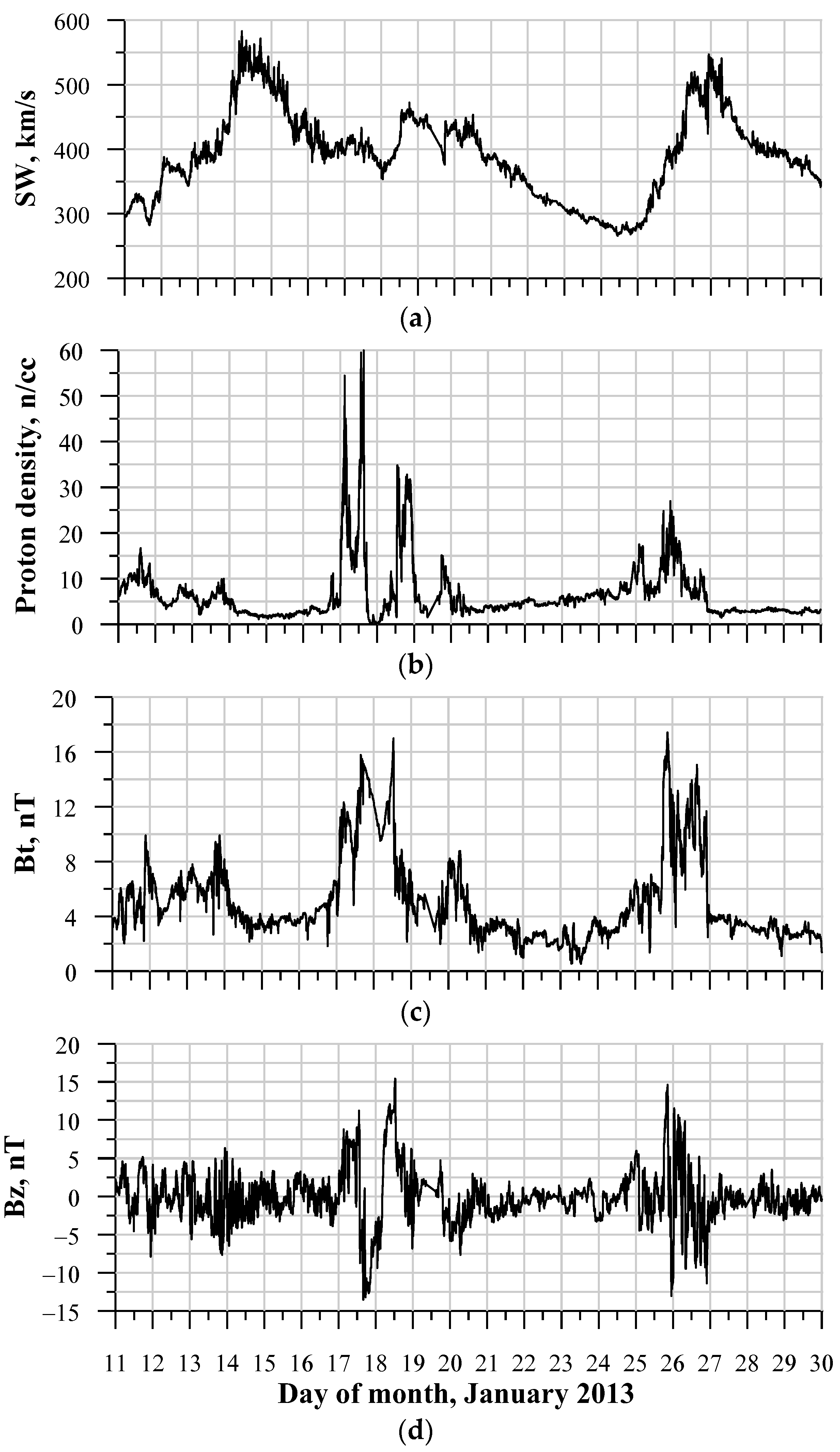
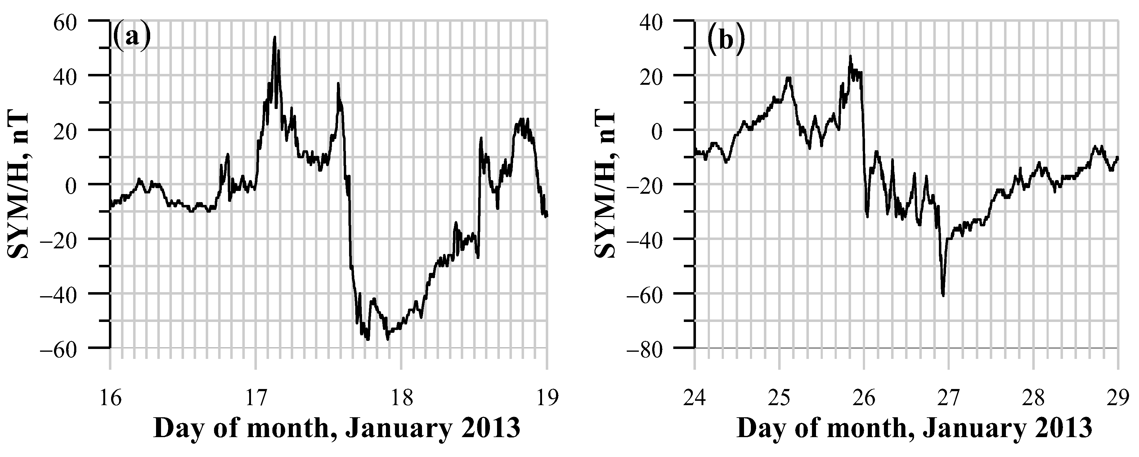
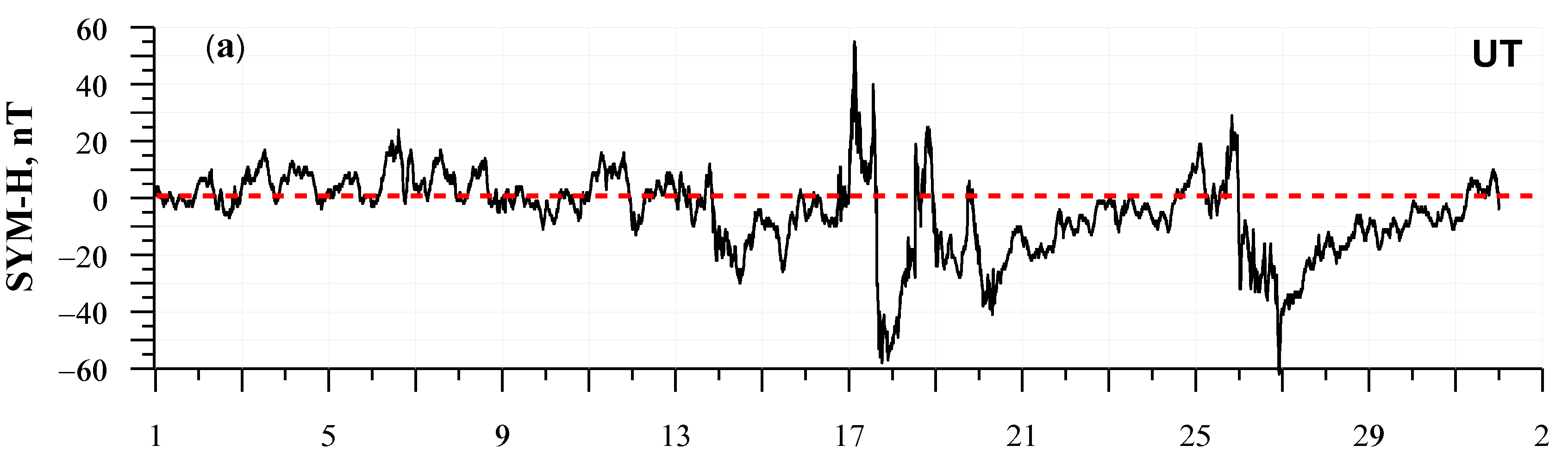
3.1. The January 2013 Solar and Geomagnetic Conditions

Variations in the parameters of the interplanetary magnetic field (IMF) for January 2013 (solar wind speed SW, proton density, total field values Bt, and vertical component Bz) are presented in Figure 1. It is shown that the IMF activity changed from a quiet level on January 11 to an active level in subsequent days with an increase in solar wind speeds (Figure 1, bottom panel) up to 590 km/sec and 579 km/sec on 14 January and 26 January, respectively, which indicated the arrival of a coronal hole high-speed stream (CH HSS). By 17 January and 26–27 January, the flow of solar wind particles was characterized by high density, and solar wind proton density was more than 10 units per cubic centimeter (cc) (Figure 1b). The total field values Bt (Figure 1c) increased to 16 nT, while Bz component values (Figure 1d) of approximately +10 nT to −14 nT indicated the arrival of the 13 January and 23 January CMEs.
The geomagnetic field responded to these changes in IMF with periods of minor storm levels on January 17 (SYM-H = −58 nT) and January 25–26 (SYM-H = −61 nT) (Figure 2). The storms were characterized by a sudden commencement (SSC or SC), marked by a sharp jump (Sudden Impuls (SI)) in the Dst values. The corresponding sudden impulses (SIs) were observed in the Boulder magnetometer at 17/0300UT (55 nT) and 25/2000UT (28 nT). The main phases of geomagnetic storms began on 17/1330UT and 25/2300UT, lasting 21 and 48 h, respectively.
The solar flux values (F10.7) shown in Figure 3 for the January 2013 period demonstrate the 27-day variation in the solar activity with enhanced F10.7 values from ~110 up to ~170 sfu. After peaking on 10 January, the solar flux values decreased to the previous level on 19–20 January.

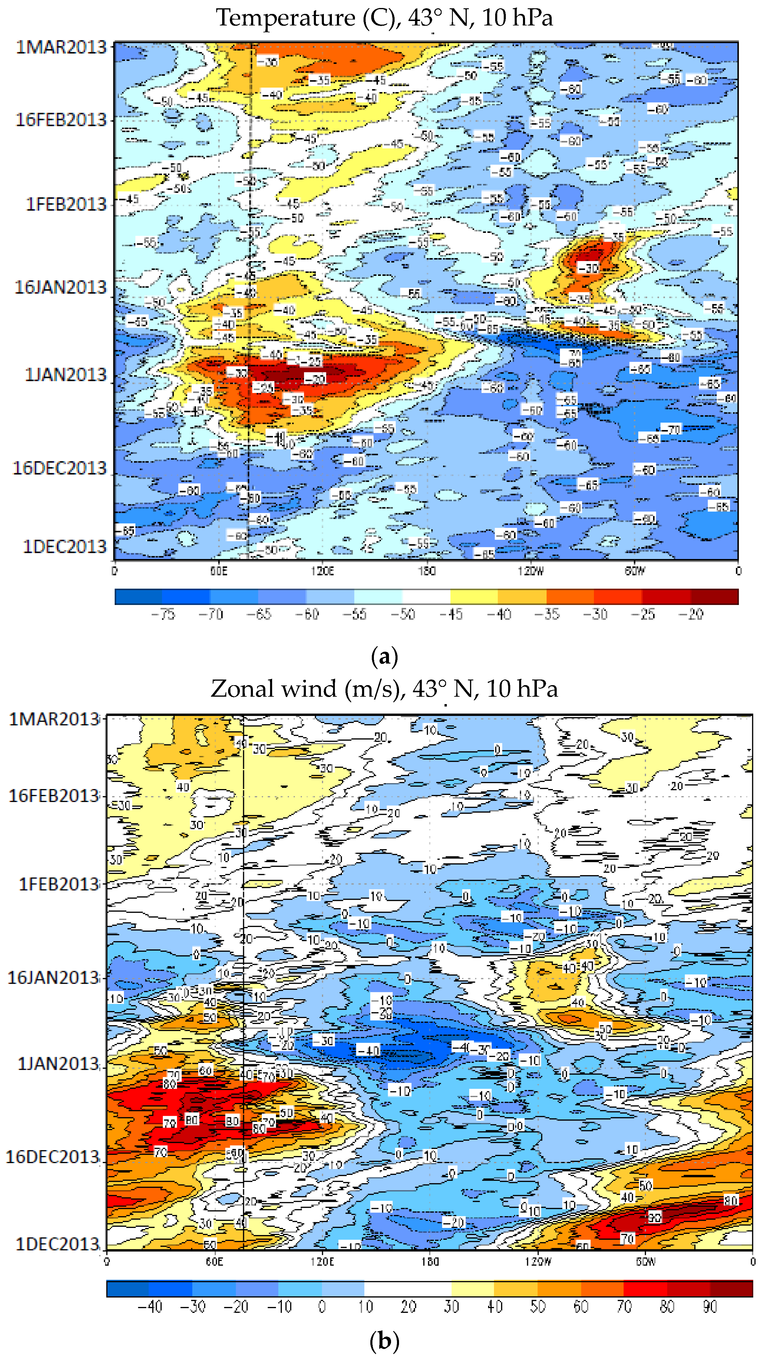
3.2. The January 2013 Major Stratospheric Warming: Temperatures and Dynamics

The SSW-2013 event in this winter has already been described in numerical studies [29,30,36,37,38,39,40,41,42,43]. Therefore, in this work, we will only briefly provide some descriptions of this event.
According to Coy and Pawson [40], the 10 hPa temperature near the North Pole (zonally averaged at 80° N) is 200 K on 1200 UTC 1 January, increasing up to 240 K by 1200 UTC 6 January for a 40 K change in 5 days. After the rapid rise, the North Pole temperature remains warm until 18 January, followed by a slower decay back to near 200 K by 10 February. The 60° N zonal mean of the zonal wind decreases as the 10 hPa polar temperature increases, changing from westerly to easterly at 1200 UTC 6 January. Coupled with the reversed 60° N to pole 10 hPa temperature gradient, this change in sign of the 10 hPa zonal mean zonal wind determined the time of the major SSW event, 1200 UTC 6 January 2013. These winds, after coming close to zero on 10 January, remain easterly until 28 January. Liu and Zhang [39] analyzed the dynamical evolution of the 2012/2013 SSW event and showed that enhanced activity of the wavenumber-2 planetary wave began in late November and early December 2012 (Figure 4), leading to a pronounced disturbance in the stratospheric polar vortex. Two additional bursts of the upward-propagating wavenumber-1 and -2 planetary waves began in mid-December and peaked on 23 December 2012 and on 5 January 2013, which led to a splitting of the stratospheric polar vortex and occurrence of easterly winds at high latitudes on 7 January 2013. After mid-January 2013, the fourth planetary wave burst which was dominated by a wavenumber-2 component occurred around January 20, leading to a persistent disturbance of the stratosphere. An example of overview of anomalies in stratospheric parameters during the November 2012 to March 2013 period is shown in Figure 4 and can be found in [36,40] (see their Figure 1).
A part of the split polar vortex displaced toward Eurasia in association with the major January 2013 SSW event, and the increased stratospheric temperature was seen within 40–60° N over the Russian Asia region [29]. The authors showed that the stratospheric temperature at a 10 hPa level (~30 km) began to rise on 21 December, and the SSW phase, related to the circulation rearrangement in the stratosphere, took place on 27 December–10 January; the zonal wind reversal at the 10 hPa level occurred on 6 January (the warming reached its peak). Figure 5a shows the seasonal march of the 10 hPa (~30 km) temperature at 43° N calculated by using the Climate Data Assimilation System (CDAS) where one can see that the temperature anomaly reaches the Almaty location, and the temperature begins to rise at the end of December 2013, reaching maximum values at the beginning of January 2013, which does not contradict observations given in [29]. The stratospheric circulation over Almaty was characterized by weekend zonal winds with two spots of easterlies in the beginning and mid-January (Figure 5b). Vertical broken lines in Figure 5 indicate the longitude of the Almaty location.
As a result, the January 2013 stratosphere warming was observed from high up to middle latitudes and characterized by numerous dynamical effects and disturbances in the temperature and wind fields caused by the SSW.
The SATI measurements were considered to provide information on the nighttime OH integral emission rates (IER) at 80–95 km. Figure 6 shows the observed OH integral emission rate (OH IER) and peak altitude of the OH layer calculated by using the nightly OH IER data and the method described by Shepherd et al. [44].
Unfortunately, the SATI data do not cover all the time intervals for the January period; there are gaps in the ground-based observations which are due to full moon or bad weather conditions when no meaningful airglow measurements are possible. However, some perturbations can be noticed in the upper mesosphere as it is reflected in the ground-based optical measurements obtained by the SATI instrument. These are quasi-periodic changes in the rate of OH emission and OH peak altitude with a quasi-period of about 6–8 days, observed in January 2013, which are possibly associated with an increase in wave activity in the stratosphere in December 2012–January 2013, as presented above. It can be seen that changes in these parameters occur synchronously: a decrease in the height of the OH IER peak corresponds to an increase in the magnitude of the OH IER on January 6–10 and 15–18, as well as an increase in the height of the OH IER peak and a decrease in the peak OH IER values on 11–14 January.

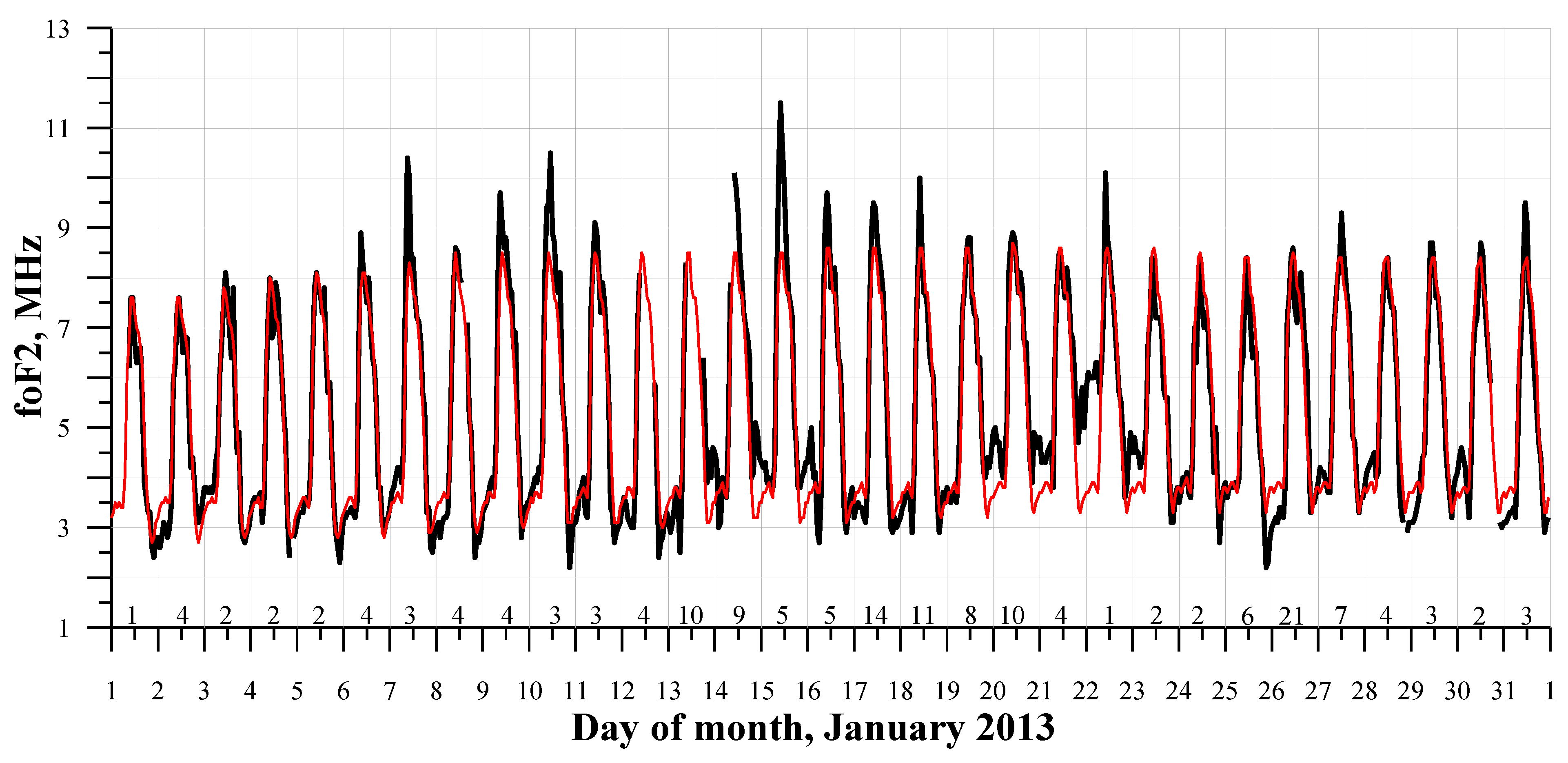
3.3. The January 2013 Dynamics of the Ionosphere

Figure 7 shows the foF2 variations observed during the January 2013 period. The most pronounced feature for the January period is a large difference between observed and running median foF2 values during 20-02LT on 13–15 and 20-06LT on 19–22 January (at night/morning local time period) when, for several hours (5–8 h), the foF2 values increased for 1.0–2.3 MHz, indicating anomalously high electron density. The daytime values are also above the running mean on 13–16 January but remain close to the median on January 19–23. These anomaly foF2 daily variations are observed under conditions of low level of geomagnetic activity;, Ap-indices for the respective days are given in the figure field, under the curves. According to commonly accepted classification (see Section 2), here Ap indices of 8 or less characterize quiet geomagnetic conditions, while Ap indices of the order of 8–15 are considered to represent unsettled geomagnetic conditions. Here, Ap indices of 6 or less characterize quiescent geomagnetic conditions. However, in this case, the variation in geomagnetic activity characterized by the Ap index does not seem to play a significant role in these enhancements since days with different Ap indices (e.g., 11 January, 17 and 31 (with Ap of 3, 14 and 3, respectively) show very similar patterns of the foF2 diurnal variations. Another example is 6 January and 26 (with Ap of 4 and 21, respectively).
The foF2 and h’F2 perturbations expressed as departures from the running medians (foF2 and h’F2) along with the Dst and OH emission rate for the whole month of the year are demonstrated in Figure 8. What is seen in the figure is the lack of the ionosphere responses to the moderate geomagnetic storms occurring on January 17 and January 26–27. The next is some wave-like variations in the foF2 and h’F with a similar quasi-period of approximately 5–8 days and foF2% values up to 60%. Moreover, the observed wave-like variations in the ionospheric parameters are quite similar to those observed in the OH emission rate (Figure 6).
The quasi-periodicity is also seen in the daily averaged foF2 values (foF2d.av.) that are shown in Figure 9 as blue crosses and the solid line. As a whole, in the beginning of January, the daily mean critical frequency has a tendency to increase in the values according to the rise in the F10.7 values (see Figure 3), assuming that the observed enhancement in foF2 can be attributed to the increase in the solar ionizing radiation flux.
But then, if the solar flux values picking around January 10 show a post-picking decrease in solar activity, the foF2d.av values continue to rise, showing that another condition is responsible for the effect. The foF2 standard deviations are smallest on 22–23 January, speaking about smallest amplitude of the foF2 diurnal variations on these days (Figure 9, red full dots and line) when the largest positive foF2 values were observed (Figure 7 and Figure 8, middle panel).
A set of original ionograms showing examples of the foF2 anomalous and typical behavior are illustrated in Figure 10 and Figure 11. They are ionograms with abnormally high F2 layer critical frequency on 21/22 January 2013 (Figure 10a–f).
At night on 22 January, the F region became strongly disturbed, spread (Figure 10d) and forked (Figure 10e) F traces indicating an appearance of different scale are observed on the ionograms in the periods that can be due to the effects of different scale irregularities and tilts in the ionosphere, which can give reflections on different frequencies with different echo delay time.
Typical ionograms for the winter ionosphere conditions are shown in Figure 11a–f which confirm that the increases in the F2 layer critical frequency observed on 21/22 January 2013 are real and foF2 is close to 6.0 MHz, whereas the typical foF2 values are between 3 and 4 MHz.
So, the observed disturbances in the F region of the ionosphere in January 2013 occurred under conditions of two moderate geomagnetic storms observed on 17 and 25–26 January (http://ftp.swpc.noaa.gov/, “URL (accessed on 16 May 2024)”, and a major sudden stratospheric warming developed in early January 2013 [36]. The observations showed: (1) No responses of the ionosphere to the 17 and 25–26 January 2013 geomagnetic storms. (2) The large foF2 (up to 60%) deviations from the running median observed at the night/morning periods on 13–15 and 19–22 January. (3) Quasi-periodic variations in the foF2, h’F, and daily averaged foF2 values occurred in January, the quasi-period of which is about 5–8 days. (4) Spread and forked F traces observed on the ionograms during night/morning periods on 13–15 and 19–22 January that can be due to the effects of different scale irregularities and tilts in the ionosphere, which can give reflections on different frequencies with different echo delay time.

4. Discussion

As shown in Section 3.1, the main phases of the January 2013 geomagnetic storms observed at the Alma-Ata station started at 13:30UT and 23:00UT, that is, at 18:00LT and 04:00LT on 17 January and 26 January 2013. The peak SYM-H values occurred at 17:00–20:00UT and 22:00UT on 17 January and 26 January; what does it mean at 22:00–04:00LT and 03:00LT on 17/18 January and 27 January, respectively. This corresponds to winter conditions and night time for this region. According to the Danilov and Lăstovička’s [5] scheme, in winter, the daytime background circulation is poleward. This leads to the effect of stopping the movement of the negative phase towards the equator, and the negative phase region is “closed to high latitudes”. But at night, these two circulations (background and storm-induced) coincide (both are directed towards the equator), and thus air with a reduced [O]/[N2] ratio spreads to low latitudes, which should lead to the appearance of a negative phase at mid-latitudes at night in winter. In our case, Figure 8 shows that a significant decrease in the foF2 values in ionospheric response to the geomagnetic storms of January 2013 was not observed. This does not mean that the above scheme does not work; perhaps under the influence of another source of disturbance the response of the ionosphere to geomagnetic storms was masked. In this case, such a masking source could be the effect on the ionosphere “from below” caused by processes associated with the major sudden stratospheric warming (SSW) event in January 2013 (see Section 3.2).
In addition, it should be noted the appearance of large (up to 60% and more) foF2 increases relative to the background level at the local night/morning hours and quasi-periodic (~6-day) variations in foF2, h’F over Almaty (see Section 3.3) during periods of increased stratospheric temperatures and easterly winds during the SSW effects in January 2013 (see Section 3.2). These results are in good agreement with Chen et al.’s [45], Mosna et al.’s [32], and Siddiqui et al.’s [33] studies. In [32,33], an increase in foF2 and the presence of wave activity were found on days of maxima of stratospheric temperature and in coincidence with the reversal zonal wind. Chen et al. [45], who studied the 2013 SSW on the meridional chain from 30.5 N to 42.8 N in northern China, showed the foF2 enhancements dominating in 8–12LT and after sunset during the 2013 SSW, and a strong ~7-day oscillation that was observed at 39.5 N and 42.8 N. The prominent “quasi-6-day wave” variations in the dayside low-latitude region, including 20–40% variations in the topside electron density and 5–10% variations in the topside total electron content (TEC), were observed by Yamazaki et al. [46] and references therein, in the ionospheric response to the September 2019 SSW, which occurred in the Southern Hemisphere. These wave-like fluctuations of ionospheric parameters with a period of less than 10 days, observed during stratospheric warmings, interpreted as planetary waves ([30,45]) or large-scale waves [46], which lead to ionospheric variability, should definitely be investigated, but this issue is beyond the scope of our present work. They can be interpreted as a manifestation of wave activity in the lower atmosphere in December 2012–January 2013.
It is difficult to say what led to compensation for the expected response of the ionosphere to geomagnetic storms (changes in stratosphere–mesosphere chemistry, ionosphere–thermosphere composition or dynamics and electrodynamics), but we can definitely say that the mechanisms accompanying SSWs influenced the development of ionospheric storms.
Of course, the explanation presented above and derived from consideration of a single event cannot explain all observations. Research [32,33], in contrast to our assumptions, showed that SSW and geomagnetic storm together strengthen their effect. Here, we can only repeat that “the global picture of ionospheric disturbances is quite complex” and can be different depending on the time of onset of the geomagnetic disturbance, season, and place of observation, demonstrating certain “portraits” of the ionospheric responses to geomagnetic field disturbances. Figure 12 illustrates several examples of differences in such “portraits” observed in winter and near-winter periods, when there was no stratospheric warming.
But at the same time, one can see a stable tendency towards the appearance of a negative phase in the change in foF2 for all the events under consideration, with the largest deviations at night. It can be assumed that a combination of the impact of several events on the ionosphere (for example, a geomagnetic storm and sudden stratospheric warming) can lead to different effects, for example, those presented in our work and in [32,33]. However, to understand the mechanism of such an effect, statistics of such observations are required, as well as model calculations (similar to [31]).

5. Conclusions

In this study, we analyzed ionospheric conditions during two minor geomagnetic storms on 17 and 26–27 January 2013 that coincided with the January major sudden stratospheric warming event that were investigated using the ionosonde and optical measurements over Almaty (Kazakhstan). The results are summarized below:
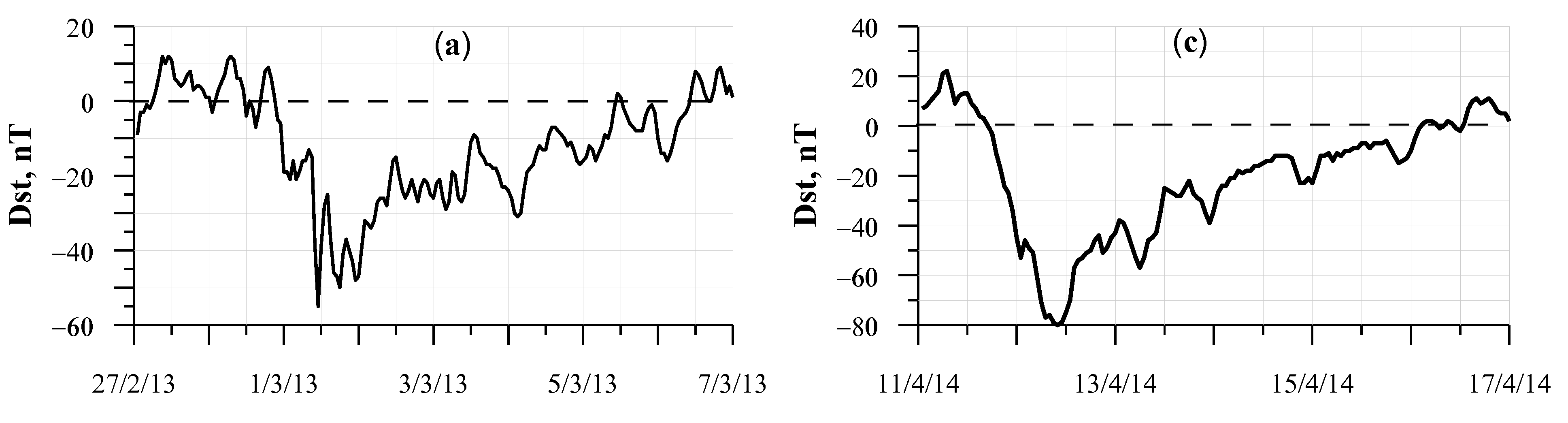
  • The ionosonde observations show no significant ionospheric storms to the 17 and 26–27 January minor (−100 < Dst < −50 nT) geomagnetic storms that indicates that the development of geomagnetic storms does not correspond to the scheme accepted in [5] for the formation of ionospheric storms during geomagnetic disturbances.
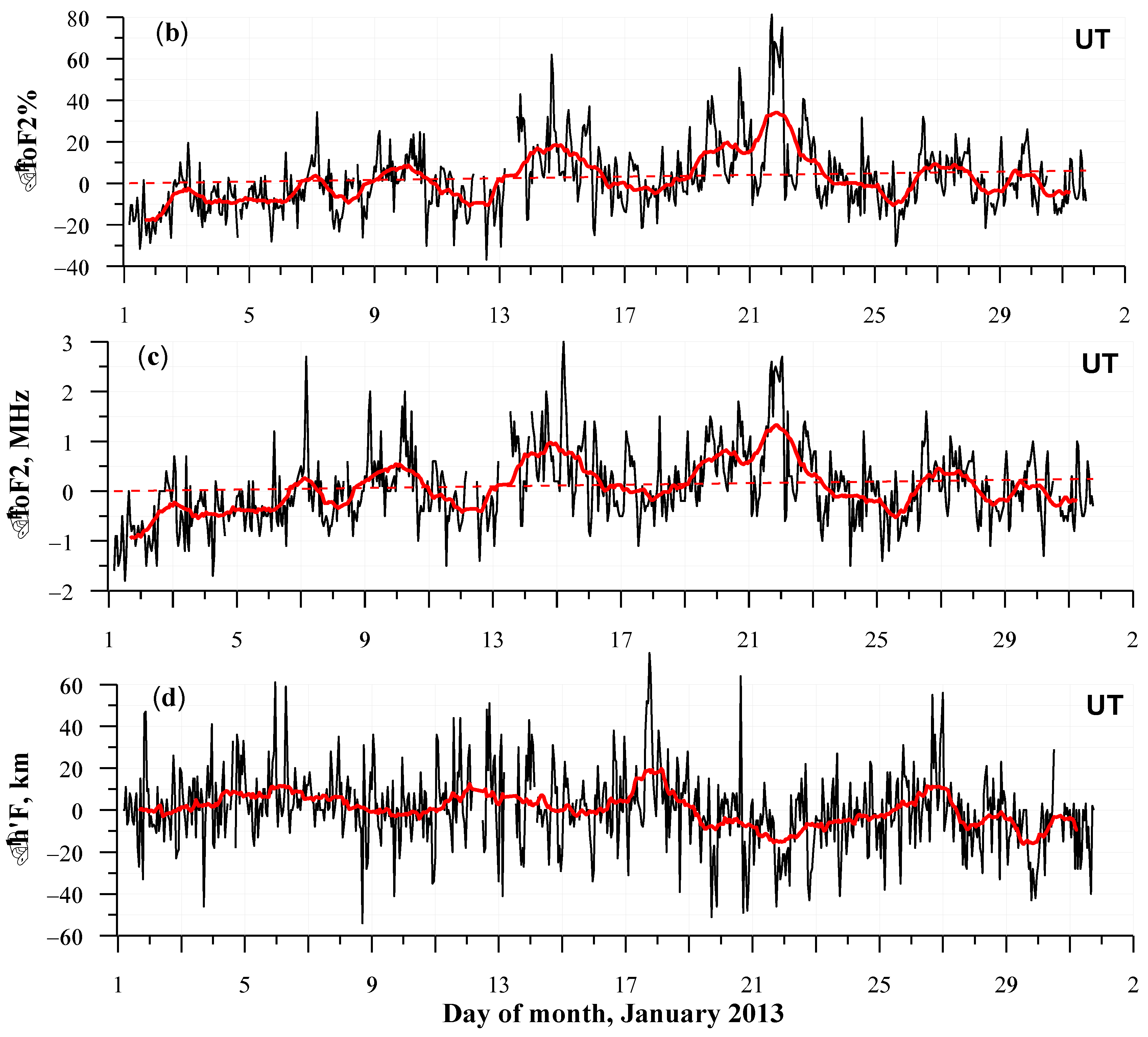
  • Large foF2 (up to 60%) deviations from the running median observed at the night/morning periods on 13–15 and 20–23 January which cannot be associated with either solar or geomagnetic activity. Spread and forked F traces observed in the ionograms at the periods indicate the appearance of different scale irregularities and tilts in the ionosphere.
  • Wave-like disturbances in ΔfoF2, Δh’F, and daily averaged foF2 values with quasi-period of 5–8 h and peak-to-peak amplitude from about 1 MHz to 2 MHz (~from 20% to ~40%) are observed during the 9–28 January period, after registration of the occurrence of the major SSW event on 6 January.
  • The observed variations in the OH emission rate are found to be quite similar to those observed in the ionospheric parameters that assume a community of processes in the stratosphere/mesosphere/ionosphere system.
It is assumed that the absence of noticeable ionospheric storms to geomagnetic disturbances indicates a change in the structure of the ionosphere and the conditions for the development of ionospheric storms caused by processes associated with the major sudden stratospheric warming recorded during this period. The latter demonstrates that the ionospheric F region is significantly influenced by processes in the lower atmosphere even under conditions of increased geomagnetic activity, similar to that concluded by Laskar et al. [30], who found “that even during high solar activity if an SSW event occurs, then the upper atmosphere is influenced significantly by lower atmospheric forcing…”.

Author Contributions

G.G. developed the data analysis methodology, interpreted the results, and drafted the manuscript. A.Y. developed the data analysis methodology, interpreted the results, and drafted the manuscript. Y.L. collected the ionosonde datasets, actively participated in the discussions on this work, and provided improvements during the preparation of the manuscript. A.A. collected the SATI datasets and provided comments on the manuscript. All authors have read and agreed to the published version of the manuscript.

Funding

Researchers GG: AYa and YuL were financially supported by the Science Committee of the Ministry of Education and Science of the Republic of Kazakhstan (project no. BR21882375), researcher AA was supported by project no. BR20280979.

Institutional Review Board Statement

Not applicable.

Informed Consent Statement

Not applicable.

Data Availability Statement

The data presented in this study are available on request from the corresponding author. The data are not publicly available due to privacy.

Conflicts of Interest

The authors declare no conflicts of interest.

References

  1. Forbes, J.M.; Palo, S.E.; Zhang, X. Variability of the ionosphere. J. Atmos. Sol.-Terr. Phys. 2000, 62, 685–693. [Google Scholar] [CrossRef]
  2. Danilov, A.D.; Morozova, L.D. Ionospheric storms in the F2 region: Morphology and physics (Review). Geomagn. Aeron. 1985, 25, 593–605. [Google Scholar]
  3. Buonsanto, M.J. Ionospheric Storms—A Review. Space Sci. Rev. 1999, 88, 563–601. [Google Scholar] [CrossRef]
  4. Mikhailov, A.V. Ionospheric F region storms. Fis. Tierra 2000, 12, 223–262. [Google Scholar]
  5. Danilov, A.D.; Lastovicka, J. Effects of geomagnetic storms on the ionosphere and atmosphere. Geomagn. Aeron. 2001, 2, 209–224. [Google Scholar]
  6. Echer, E.; Gonzalez, W.D.; Tsurutani, B.T. Interplanetary conditions leading to superintense geomagnetic storms (Dst 250 nT) during solar cycle 23. Geophys. Res. Lett. 2008, 35, L06S03. [Google Scholar] [CrossRef]
  7. Echer, E.; Gonzalez, W.D.; Tsurutani, B.T. Statistical studies of geomagnetic storms with peak Dst 50 nT from 1957 to 2008. J. Atmos. Sol.-Terr. Phys. 2011, 73, 1454–1459. [Google Scholar] [CrossRef]
  8. Paznukhov, V.V.; Altadill, D.; Reinisch, B.W. Experimental evidence for the role of the neutral wind in the development of ionospheric storms in midlatitudes. J. Geophys. Res. 2009, 114, A12319. [Google Scholar] [CrossRef]
  9. Danilov, A.D. Ionospheric F-region response to geomagnetic disturbances. Adv. Space Res. 2013, 52, 343–366. [Google Scholar] [CrossRef]
  10. Perrone, L.; Mikhailov, A.V.; Sabbagh, D. Thermospheric Parameters during Ionospheric G-Conditions. Remote Sens. 2021, 13, 3440. [Google Scholar] [CrossRef]
  11. Gordiyenko, G. Ionospheric response over the Middle Asian region to the May 1967 geomagnetic storm. J. Atmos. Sol.-Terr. Phys. 2023, 253, 106151. [Google Scholar] [CrossRef]
  12. Gordienko, G.I.; Vodyannikov, V.V.; Yakovets, A.F. Geomagnetic storm effects in the ionospheric E- and F-regions. J. Atmos. Sol.-Terr. Phys. 2011, 73, 1818–1830. [Google Scholar] [CrossRef]
  13. Cander, L.R. Mid-Latitude Single Station F region Storm Morphology and Forecast. Acta Geophys. 2016, 64, 541–566. [Google Scholar] [CrossRef]
  14. Matsuno, T.A. Dynamical Model of the Stratospheric Sudden Warming. J. Atmos. Sci. 1971, 28, 1479–1494. [Google Scholar] [CrossRef]
  15. Charlton, A.J.; Polvani, L.M. A New Look at Stratospheric Sudden Warmings. Part I: Climatology and Modeling Benchmarks. J. Clim. 2007, 20, 449–469. [Google Scholar] [CrossRef]
  16. Nath, D.; Chen, W.; Zelin, C.; Pogoreltsev, A.I.; Wei, K. Dynamics of 2013 Sudden Stratospheric Warming event and its impact on cold weather over Eurasia: Role of planetary wave Reflection. Sci. Rep. 2016, 6, 24174. [Google Scholar] [PubMed]
  17. Pedatella, N.M.; Chau, J.L.; Schmidt, H.; Goncharenko, L.P.; Stolle, C.; Hocke, K.; Harvey, V.L.; Funke, B.; Siddiqui, T.A. How sudden stratospheric warming affects the whole atmosphere. EOS 2018, 99, 35–38. [Google Scholar] [CrossRef]
  18. Baldwin, M.P.; Ayarzagüena, B.; Birner, T.; Butchart, N.; Butler, A.H.; Charlton-Perez, A.J.; Domeisen, D.I.V.; Garfinkel, C.I.; Garny, H.; Gerber, E.P.; et al. Sudden Stratospheric Warmings. Rev. Geophys. 2021, 59, e2020RG000708. [Google Scholar] [CrossRef]
  19. Goncharenko, L.P.; Chau, J.L.; Liu, H.L.; Coster, A.J. Unexpected connections between the stratosphere and ionosphere. Geophys. Res. Lett. 2010, 37, L10101. [Google Scholar] [CrossRef]
  20. Goncharenko, L.; Zhang, S.R. Ionospheric signatures of sudden stratospheric warming: Ion temperature at middle latitude. Geophys. Res. Lett. 2008, 35, L21103. [Google Scholar] [CrossRef]
  21. Chau, J.L.; Fejer, B.G.; Goncharenko, L.P. Quiet variability of equatorial E × B drifts during a sudden stratospheric warming event. Geophys. Res. Lett. 2009, 36, L05101. [Google Scholar] [CrossRef]
  22. Yue, X.; Schreiner, W.S.; Lei, J.; Rocken, C.; Hunt, D.C.; Kuo, Y.-H.; Wan, W. Global ionospheric response observed by COSMIC satellites during the January 2009 stratospheric sudden warming event. J. Geophys. Res. 2010, 115, A00G09. [Google Scholar] [CrossRef]
  23. Shepherd, M.G.; Shepherd, G.G. Stratospheric warming effects on thermospheric O(1S) dayglow dynamics. J. Geophys. Res. 2011, 116, A11327. [Google Scholar] [CrossRef]
  24. Pancheva, D.; Mukhtarov, P. Stratospheric warmings: The atmosphere–ionosphere coupling paradigm. J. Atmos. Sol.-Terr. Phys. 2011, 73, 1697–1702. [Google Scholar] [CrossRef]
  25. Bessarab, F.S.; Korenkov, Y.N.; Klimenko, M.V.; Klimenko, V.V.; Karpov, I.V.; Ratovsky, K.G.; Chernigovskaya, M.A. Modeling the effect of sudden stratospheric warming within the thermosphere-ionosphere system. J. Atmos. Sol.-Terr. Phys. 2012, 90–91, 77–85. [Google Scholar] [CrossRef]
  26. Sumod, S.G.; Pant, T.K.; Jose, L.; Hossain, M.M.; Kumar, K.K. Signatures of Sudden Stratospheric Warming on the Equatorial Ionosphere-Thermosphere System. Planet. Space Sci. 2012, 63–64, 49–55. [Google Scholar] [CrossRef]
  27. Fang, T.W.; Fuller-Rowell, T.; Akmaev, R.; Wu, F.; Wang, H.; Anderson, D. Longitudinal variation of ionospheric vertical drifts during the 2009 sudden stratospheric warming. J. Geophys. Res. 2012, 117, A03324. [Google Scholar] [CrossRef]
  28. Polekh, N.M.; Kurkin, V.I.; Zolotukhina, N.A.; Chernigovskaya, M.A. On the connection between nighttime winter ionization increase in midlatitude F region and stratosphere warming. Sol.-Terr. Phys. 2013, 22, 41–46. (In Russian) [Google Scholar]
  29. Polyakova, A.S.; Chernigovskaya, M.A.; Perevalova, N.P. Ionospheric effects of sudden stratosperic warmings in eastern Siberia region. J. Atmos. Sol.-Terr. Phys. 2014, 120, 15–23. [Google Scholar] [CrossRef]
  30. Laskar, F.I.; Pallamraju, D.; Veenadhari, B. Vertical coupling of atmospheres: Dependence on strength of sudden stratospheric warming and solar activity. Earth Planets Space 2014, 66, 94. [Google Scholar] [CrossRef]
  31. Pedatella, N.M. Impact of the lower atmosphere on the ionosphere response to a geomagnetic superstorm. Geophys. Res. Lett. 2016, 43, 9383–9389. [Google Scholar] [CrossRef]
  32. Mošna, Z.; Edemskiy, I.; Laštovička, J.; Kozubek, M.; Koucká Knížová, P.; Kouba, D.; Siddiqui, T.A. Observation of the Ionosphere in Middle Latitudes during 2009, 2018 and 2018/2019 Sudden Stratospheric Warming Events. Atmosphere 2021, 12, 602. [Google Scholar] [CrossRef]
  33. Siddiqui, T.A.; Yamazaki, Y.; Stolle, C.; Maute, A.; Laštovička, J.; Edemskiy, I.K.; Mošna, Z.; Sivakandan, M. Understanding the total electron content variability over Europe during 2009 and 2019 SSWs. J. Geophys. Res. Space Phys. 2021, 126, e2020JA028751. [Google Scholar] [CrossRef]
  34. Karpenko, A.L.; Leshchenko, L.N.; Manaenkova, N.I. Peculiarities and perspectives of network digital ionospheric station ‘‘PARUS”. In Proceedings of the Progress in Electromagnetics Research (PIERS) Symposium Proceedings 2009, Moscow, Russia, 18–21 August 2009; pp. 219–222. [Google Scholar]
  35. Sargoytchev, S.; Brown, S.; Solheim, B.; Cho, Y.-M.; Shepherd, G.; López-Gonzàlez, M.-J. Spectral Airglow Temperature Imager (SATI)—A ground based instrument for temperature monitoring of the mesosphere region. Appl. Opt. 2004, 43, 5712. [Google Scholar] [CrossRef] [PubMed]
  36. Goncharenko, L.; Chau, J.L.; Condor, P.; Coster, A.; Benkevitch, L. Ionospheric effects of sudden stratospheric warming during moderate-to-high solar activity: Case study of January 2013. Geophys. Res. Lett. 2013, 40, 4982–4986. [Google Scholar] [CrossRef]
  37. Goncharenko, L.P.; Coster, A.J.; Zhang, S.R.; Erickson, P.J.; Benkevitch, L.; Aponte, N.; Harvey, V.L.; Reinisch, B.W.; Galkin, I.; Spraggs, M.; et al. Deep ionospheric hole created by sudden stratospheric warming in the nighttime ionosphere. J. Geophys. Res. Space Phys. 2018, 123, 7621–7633. [Google Scholar] [CrossRef]
  38. Laskar, F.I.; McCormack, J.P.; Chau, J.L.; Pallamraju, D.; Hoffmann, P.; Singh, R.P. Interhemispheric meridional circulation during sudden stratospheric warming. J. Geophys. Res. Space Phys. 2019, 124, 7112–7122. [Google Scholar] [CrossRef]
  39. Liu, Y.; Zhang, Y. Overview of the major 2012–2013 Northern Hemisphere stratospheric sudden warming: Evolution and its association with surface weather. J. Meteor. Res. 2014, 28, 561–575. [Google Scholar] [CrossRef]
  40. Coy, L.; Pawson, S. The Major Stratospheric Sudden Warming of January 2013: Analyses and Forecasts in the GEOS-5 Data Assimilation System. Mon. Weather. Rev. 2015, 143, 491–510. [Google Scholar] [CrossRef]
  41. De Wit, R.J.; Hibbins, R.E.; Espy, P.J.; Orsolini, Y.J.; Limpasuvan, V.; Kinnison, D.E. Observations of gravity wave forcing of the mesopause region during the January 2013 major Sudden Stratospheric Warming. Geophys. Res. Lett. 2014, 41, 4745–4752. [Google Scholar] [CrossRef]
  42. Shpynev, B.G.; Kurkin, V.I.; Ratovsky, K.G.; Chernigovskaya, M.A.; Belinskaya, A.Y.; Grigorieva, S.A.; Stepanov, A.E.; Bychkov, V.V.; Pancheva, D.; Mukhtarov, P. High-midlatitude ionosphere response to major stratospheric warming. Earth Planets Space 2015, 67, 18. [Google Scholar] [CrossRef]
  43. Yasyukevich, A.S.; Kulikov, Y.Y.; Klimenko, M.V.; Klimenko, V.V.; Bessarab, F.S.; Korenkov, Y.N.; Marichev, V.N.; Ratovsky, K.G.; Kolesnik, S.A. Changes in the stratosphere and ionosphere parameters during the 2013 major stratospheric warming. Sol.-Terr. Phys. 2018, 4, 48–58. [Google Scholar] [CrossRef]
  44. Shepherd, M.G.; Cho, Y.M.; Shepherd, G.G.; Ward, W.; Drummond, J.R. Mesospheric temperature and atomic oxygen response during the January 2009 major stratospheric warming. J. Geophys. Res. 2010, 115, A07318. [Google Scholar] [CrossRef]
  45. Chen, G.; Wu, C.; Zhang, S.; Ning, B.; Huang, X.; Zhong, D.; Qi, H.; Wang, J.; Huang, L. Midlatitude ionospheric responses to the 2013 SSW under high solar activity. J. Geophys. Res. Space Phys. 2016, 121, 790–803. [Google Scholar] [CrossRef]
  46. Yamazaki, Y.; Matthias, V.; Miyoshi, Y.; Stolle, C.; Siddiqui, T.; Kervalishvili, G.; Laštovička, J.; Kozubek, M.; Ward, W.; Themens, D.R.; et al. September 2019 Antarctic sudden stratospheric warming: Quasi-6-Dday wave burst and ionospheric effects. Geophys. Res. Lett. 2020, 47, e2019GL086577. [Google Scholar] [CrossRef]
Figure 1. Solar wind speed SW (a), Proton density (b), total field values Bt (c), and vertical component Bz (d) for the period 11–29 January 2013.
Atmosphere 15 00626 g001
Figure 2. SYM-H data for 16–18 January (a) and 24–28 January 2013 (b).
Atmosphere 15 00626 g002
Figure 3. Solar flux F10.7 and Ap indexes for January 2013.
Atmosphere 15 00626 g003
Figure 4. Evolution of the daily values from 1 November 2012 to 1 April 2013 of 100 hPa eddy heat flux averaged between 45 and 75° N for zonal wavenumber-1 (blue dashed line), wavenumber-2 (red dotted line), and the sum of the first three wavenumbers (black solid line). The dashed vertical line indicates the peak date of the 10 hPa temperature at the North Pole on 7 January 2013 (Figure 1c from [39]).
Atmosphere 15 00626 g004
Figure 5. (a). Longitudinal evolution of the 10 hPa temperature (a) and zonal wind (b) at 43° N for the period from December to February 2013 (Climate Assimilation System, CDAS). Vertical broken line indicates the longitude of the Almaty location. (b). The same as in Figure 5a but only for zonal wind.
Atmosphere 15 00626 g005
Figure 6. The OH airglow integral emission rate (a) and OH IER peak altitude (b) for January 2013. Full dots—observed values, red crosses—nightly averaged, blue line—9-degree polynomial fitting.
Atmosphere 15 00626 g006
Figure 7. The foF2 diurnal variations as observed at Alma-Ata station during 1–31 January 2013 (thick line). The running median (L = 27) is used as a reference and is shown as a thin line. The Ap indices for the respective days are given under the curves.
Atmosphere 15 00626 g007
Figure 8. Variations in SYM-H (a), ΔfoF2% (b), ΔfoF2 (c) and Δh’F (d) in January 2013.
Atmosphere 15 00626 g008aAtmosphere 15 00626 g008b
Figure 9. Diurnal averaged foF2 values (crosses, blue line) and the foF2 standard deviations (filled circles, red line) for Jan. 2013.
Atmosphere 15 00626 g009
Figure 10. A number of typical ionograms for winter nighttime ionospheric conditions, as was observed at the Alma-Ata station from 23LT to 06LT on 21/22 January 2013. 23:10LT (a), 00:00LT (b), 01:00LT (c), 02:40LT (d), 04:00LT (e), 05:30LT (f).
Atmosphere 15 00626 g010
Figure 11. Typical ionograms observed in January from 23LT to 06LT on 23/24 January 2013. 23:10LT (a), 00:00LT (b), 01:30LT (c), 02:40LT (d), 04:00LT (e), 05:30LT (f).
Atmosphere 15 00626 g011
Figure 12. Examples of changes in the critical frequency of the F2 layer during geomagnetic disturbances over the Alma-Ata station. 27 February 2013–6 March 2013 (a,b), 11–16 April 2014 (c,d), 30 December 2015–4 January 2016 (e,f), 1–6 April 2016 (g,h).
Atmosphere 15 00626 g012aAtmosphere 15 00626 g012b
Disclaimer/Publisher’s Note: The statements, opinions and data contained in all publications are solely those of the individual author(s) and contributor(s) and not of MDPI and/or the editor(s). MDPI and/or the editor(s) disclaim responsibility for any injury to people or property resulting from any ideas, methods, instructions or products referred to in the content.

