Mid- and High-Latitude Electron Temperature Dependence on Solar Activity in the Topside Ionosphere through the Swarm B Satellite Observations and the International Reference Ionosphere Model

Abstract

This study focuses on the open question of the electron temperature (T_e) variation with solar activity in the topside ionosphere at mid- and high latitudes. It takes advantage of in situ observations taken over a decade (2014–2023) from Langmuir probes on board the low-Earth-orbit Swarm B satellite and spanning an altitude range of 500–530 km. The study also includes a comparison with T_e values modeled using the International Reference Ionosphere (IRI) model and with Millstone Hill (42.6° N. 71.5° W) incoherent scatter radar observations. The largest T_e variation with solar activity was found at high latitudes in the winter season, where T_e shows a marked decreasing trend with solar activity in the polar cusp and auroral regions and, more importantly, at sub-auroral latitudes in the nightside sector. Differently, in the summer season, T_e increases with solar activity in the polar cusp and auroral regions, while for equinoxes, variations are smaller and less clear. Mid-latitudes generally show negligible T_e variations with solar activity, which are mostly within the natural dispersion of T_e observations. The comparison between measured and modeled values highlighted that future implementations of the IRI model would benefit from an improved description of the T_e dependence on solar activity, especially at high latitudes.

1. Introduction

An accurate description of the electron temperature (T_e) variations with solar activity in the topside ionosphere is still not fully achieved and is, thus, worthy of deeper investigation based on the data gathered from the most recent and state-of-the-art low-Earth-orbit (LEO) satellite missions. A better description of the T_e variations with solar activity would be of benefit not only for empirical and physics-based ionospheric models but also for LEO satellite designers and engineers, with the topside ionosphere being the medium in which these satellites fly.

The topside ionosphere includes plasma in the region extending from the F2-layer peak, which is the electron density (N_e) absolute maximum of the ionosphere at an altitude of about 250–450 km from the ground, to the overlying plasmasphere or plasma trough at high and polar latitudes. The border between the ionosphere and plasmasphere, which is considered to be the so-called upper transition height, is very variable with space, time, and solar activity level [1], ranging from about 450 km of altitude at night for low solar activity [2], to about 1600 km [3] or even 2000 km [4] at daytime for high solar activity. The topside ionosphere is a highly dynamic region characterized by a monotonic decrease in N_e with altitude, accompanied by a monotonic increase in T_e, with a vertical rate of change strongly dependent on the geophysical conditions for both plasma parameters. Such altitudinal variations are driven by the plasma ambipolar diffusion along geomagnetic field lines [5,6], and variations in both physical and chemical plasma parameters are driven by the interaction with solar radiation, solar wind, and neutral atmosphere [7,8]. Moreover, for most of the conditions, in the topside ionosphere, the temperatures of the diverse ionospheric plasma components (i.e., electrons and ions) and neutrals are not in thermal equilibrium [9], with T_e exceeding the temperature of ions (T_i) and neutrals (T_n) and showing much faster variations because of the much lower mass of electrons compared to that of ions and neutrals [10]. To make the description of T_e more complicated, there is also its strict coupling with N_e through the electron conservation energy equation [11], where both N_e and T_e affect the plasma distribution function and concur with the energetic balance of the ionospheric plasma. All these processes make the description of T_e in the ionosphere a rather complex problem.

Since the 1960s, the availability of T_e remote sensing observations from ground-based incoherent scatter radars (ISRs) and in situ T_e observations from Langmuir probes (LPs) and retarding potential analyzers (RPAs) on board LEO satellites [12] allowed for the description of the main large-scale time and spatial features of T_e in the ionosphere. The wealth of information collected in recent decades allowed for the implementation of empirical global models of T_e [13,14,15], on which the International Reference Ionosphere (IRI) model [16] relies. IRI is the empirical climatological ionosphere model of reference for the ionospheric community and describes the median behavior of plasma parameters, including T_e, on a global basis and for different levels of solar and magnetic activity. IRI evolves and improves with time because of the ever-growing availability of new observations to be included in its underlying dataset, and the development of new modeling techniques. The current default option for the T_e modeling in the last version of IRI, i.e., IRI-2020 [16], is based on the works by Truhlik et al. [15,17,18] and also includes the dependence on solar activity. In previous work, Pignalberi et al. [19] compared IRI-modeled T_e with corresponding values observed by the three Swarm satellites for the years 2014–2020, and with observations made by Arecibo, Jicamarca, and Millstone Hill ISRs. That comparison allowed for the evaluation of the IRI model’s ability to predict the large-scale median variations in T_e in the topside ionosphere (450–520 km), as a function of latitude, longitude, local time, and season. However, the T_e variations with solar activity were not addressed. The present study aims to fill this gap.

Besides the validation of the T_e modeling from IRI, the T_e variation with solar activity in the topside ionosphere is itself an issue yet to be solved. Section 2 sets the historical background on the topic based on studies performed from the 1960s on. These studies highlighted the complexity of the T_e dependence on solar activity. Indeed, T_e showed variations with solar activity that are critically dependent on the considered altitude, latitude, local time, and season. Therefore, to properly extract statistically robust information on the T_e dependence on solar activity, the altitudinal, latitudinal, local time, and seasonal variations have to be specified.

The European Space Agency’s (ESA) Swarm LEO satellites offer the opportunity to investigate this issue in unprecedented detail. This is made possible through ten years, from the beginning of 2014 to the end of 2023, of in situ T_e observations made by LPs on board Swarm satellites. This study focuses on the Swarm B satellite which covered the altitude range 500–530 km, and the mid- and high latitudes, specifically from 30° Quasi-Dipole (QD) geomagnetic latitude to the geomagnetic poles, for both hemispheres. The reason for this choice has both scientific and instrumental motivations. Indeed, results from previous studies highlighted that, concerning the Swarm B altitude range, the largest T_e variations with solar activity occur at mid- and high latitudes. Moreover, and more importantly for this study, under high solar activity conditions at low latitudes, Swarm LP data show some features, as detailed in Section 3.1, that need further investigation before being used to extract accurate information on the T_e variation with solar activity.

Section 3 describes the Swarm B dataset, the Millstone Hill ISR observations, and the IRI T_e model. The T_e variations with solar activity are shown in Section 4, for both Swarm B-measured and IRI-modeled T_e values. Section 5 discusses the results in light of the current knowledge of the physical processes involving the topside ionosphere plasma and its coupling with the plasmasphere and the magnetosphere. The same section discusses the implications that this study has on the T_e modeling using IRI. Finally, Section 6 draws the conclusions and possible future developments.

2. Historical Background

A number of authors investigated the T_e variations with solar activity in the ionosphere based on observations made from different facilities, using different instruments, and applying different analysis techniques. The corresponding results in some cases are different, if not conflicting.

A first investigation by Brace et al. [20], through Explorer-22 satellite T_e observations at about 1000 km for the years 1965–1967 (ascending part of the 20th solar cycle), showed a daytime T_e increase with solar activity in the years 1965 and 1966 but a marked decrease in 1967 despite the increasing solar activity. The same study also showed a nighttime T_e increase with solar activity in the years 1965 and 1966, which was, however, not so clear between 1966 and 1967 under higher solar activity.

Through early observations from Millstone Hill (42.6° N. 71.5° W) ISR between 1964 and 1968, Evans [21] found that the seasonal variation in T_e at 300 km and 500 km shows a complex dependence on solar activity and local time. Specifically, at Millstone Hill for daytime conditions, the summer T_e exceeds the winter T_e by an amount that increases with solar activity. Differently, nighttime T_e, which is instead greater in winter than in summer, shows no variation with solar activity.

Mahajan and Pandey [22] complemented the study by Brace et al. [20] by including T_e observations at 1000 km from the ISIS-1 satellite for the years 1969 and 1970 (maximum of the 20th solar cycle). They found a T_e increase with solar activity at all latitudes for both daytime and nighttime conditions.

One of the first comprehensive investigations of the global median behavior of T_e in the ionosphere was provided by Brace and Theis [14], who described the main T_e variations at the altitudes of 300 km, 400 km, 1400 km, and 3000 km through in situ observations recorded by the ISIS-1 and -2 and Atmospheric Explorer-C (AE-C) satellites from 1969 to 1978. They modeled T_e at these altitudes through spherical harmonic expansions as a function of dip latitude, local time, and season, without introducing any solar activity dependence. By studying how the ratios between measured and modeled T_e values behave as a function of solar activity, they concluded that there is little variation with the solar activity at 400 km and 3000 km for daytime conditions at mid-latitudes. For the same conditions, they found a T_e decrease of the order of 20% for high solar activity at 300 km. Instead, at 300 km for nighttime conditions at equatorial latitudes, they found a clear increase in T_e with solar activity. Although they realized that the T_e variation with solar activity is a second-order effect after altitudinal, latitudinal, and local time variations, they also highlighted that the dependence on solar activity is strongly affected by altitude, latitude, and local time, in a complex way.

Brace et al. [23] compared the Dynamics Explorer-2 (DE-2) and AE-C in situ observations between 300 km and 400 km, recorded at high and low solar activity during the daytime. While they found a clear increase in N_e with solar activity, for the same conditions, T_e differed only in detail and with a clear dependence on magnetic latitude.

The dependence on the magnetic latitude of the T_e variation with solar activity was further investigated by Brace et al. [24] through the DE-2 and AE-C in situ observations between 300 km and 400 km from 1973 to 1983. For daytime conditions, they highlighted an increase in T_e with solar activity with a rate of change maximizing at the geomagnetic equator and decreasing towards the poles.

Bilitza and Hoegy [25] reviewed past studies on the T_e variation with solar activity and added new insights based on Arecibo (18.2° N, 66.4° W) ISR observations at 400 km from 1966 to 1984, for daytime and nighttime conditions. Akin to the results found by [21] with the Millstone Hill ISR data, also at Arecibo, Bilitza and Hoegy [25] found that the T_e seasonal variation is larger than that of the solar activity, but with marked seasonal differences compared to Millstone Hill. Indeed, for daytime conditions, while observations at Millstone Hill showed a T_e increase with solar activity during summer and a decrease in winter, observations at Arecibo showed the opposite trend. Differently, for nighttime conditions, T_e showed a slightly increasing trend with solar activity at both Arecibo and Millstone Hill and for both the summer and winter seasons.

Brace and Theis [26] also included the solar activity variation in their global models of T_e at 300 km, 500 km, and 850 km, and interpolated between anchor points at different altitudes through a quadratic function. By comparing global T_e maps modeled at 400 km at different solar activity levels for the March equinox, they found that T_e showed little variation with solar activity compared to N_e, with similar latitudinal and local time patterns (in geomagnetic coordinates) across different solar activity levels. At a 60° geomagnetic latitude, T_e showed the highest values for low solar activity, especially during the daytime. Differently, at 30° and 0° geomagnetic latitudes, T_e showed a less defined pattern with solar activity, with an increase or a decrease at different local times.

Otsuka et al. [27] studied the T_e variations in the range of 200–550 km through observations recorded by the Shigaraki (34.8°N, 136.1°E) ISR from 1986 to 1995. They found that daytime T_e decreases with solar activity, while nighttime T_e increases with solar activity.

Sethi et al. [28] studied the T_e variation with solar activity in the range of 100–700 km through the Arecibo ISR observations. They found that in the F region (200–350 km), T_e increases with solar activity, while in the topside (400–700 km), T_e shows little variation with solar activity, which highlights how the T_e variation with solar activity is strongly dependent on altitude.

Zhang and Holt [29] found a definite dependence on altitude in the solar activity variation in T_e by analyzing the Millstone Hill ISR observations from 1976 to 2001 and associated it with the corresponding N_e variation. Such results were also confirmed by Lei et al. [30], who analyzed observations from the Arecibo and Millstone Hill ISRs and compared them with corresponding values modeled by the TIE-CGM physics-based model. At Millstone Hill, they found that the daytime T_e increases with solar activity in the bottomside ionosphere (below the F2-layer peak) for all seasons, while in summer, the increase also involves the topside ionosphere. At nighttime, T_e generally increases with solar activity in equinoxes and summer. At Arecibo, they found that nighttime T_e generally increases with solar activity, while daytime T_e behaves in a more complex way, increasing clearly with solar activity only in the bottomside. In the topside, slight T_e increases with solar activity were found at equinoxes and in summer. Lei et al. [30] related the complex dependence of T_e on solar activity to the corresponding variations in N_e and T_n.

Bilitza et al. [31] extensively investigated the T_e variation with solar activity for mid-latitudes at 550 km, 850 km, and 2000 km of altitude for different seasons and for daytime and nighttime conditions, through a large collection of in situ observations from different LEO satellites from 1964 to 2005. They highlighted that at mid-latitudes, T_e can increase, decrease, or be constant with solar activity depending on altitude, local time, and season. Specifically, they found that at 550 km and during the daytime, T_e increases with solar activity in summer and decreases at equinoxes, with negligible variations in the winter. During the nighttime at 550 km, the trend reverses in summer and at equinoxes, while in winter, the T_e variations are negligible. At 850 km, T_e showed a decreasing trend with solar activity for winter and equinoxes for daytime conditions, a slightly increasing trend for summer nighttime conditions, and negligible variations in the other cases. At 2000 km, a general decreasing trend is observed except for in winter daytime conditions.

Truhlik et al. [32] extended the study by Bilitza et al. [31] by investigating the latitudinal variation in T_e for different solar activity levels and including the altitude of 1400 km in addition to the altitudes studied by [31]. Truhlik et al. [32] highlighted that at equinoxes, T_e generally increases with solar activity except at 550 km for daytime conditions. Differently, at solstices, the T_e dependence on solar activity is more detailed. At 550 km and for daytime conditions, T_e increases with solar activity in the summer hemisphere while the opposite trend is seen in the winter hemisphere, and these trends maximize in amplitude towards high latitudes, while they are negligible at low latitudes. Differently, at 550 km, but for nighttime conditions, T_e shows a slightly increasing trend with solar activity across different latitudes and seasons. Overall, Truhlik et al. [32] highlighted how at 550 km of altitude, T_e shows a complex dependence on solar activity, which is significantly affected by the latitude, local time, and season.

Stolle et al. [33] found a negative correlation between the amplitude of the morning overshoot in T_e and the solar flux at an altitude of 340 km using the data from the CHAMP satellite. This result was supported by the data from the Jicamarca ISR and agreed well with calculations from the physics-based FLIP model.

Leveraging the achievements by [31,32], Truhlik et al. [15] introduced the solar activity variation in the IRI T_e modeling. This is the default option for T_e modeling in the current IRI version, i.e., IRI-2020, and will be extensively described in Section 3.2.

3. Data, Models, and Methods

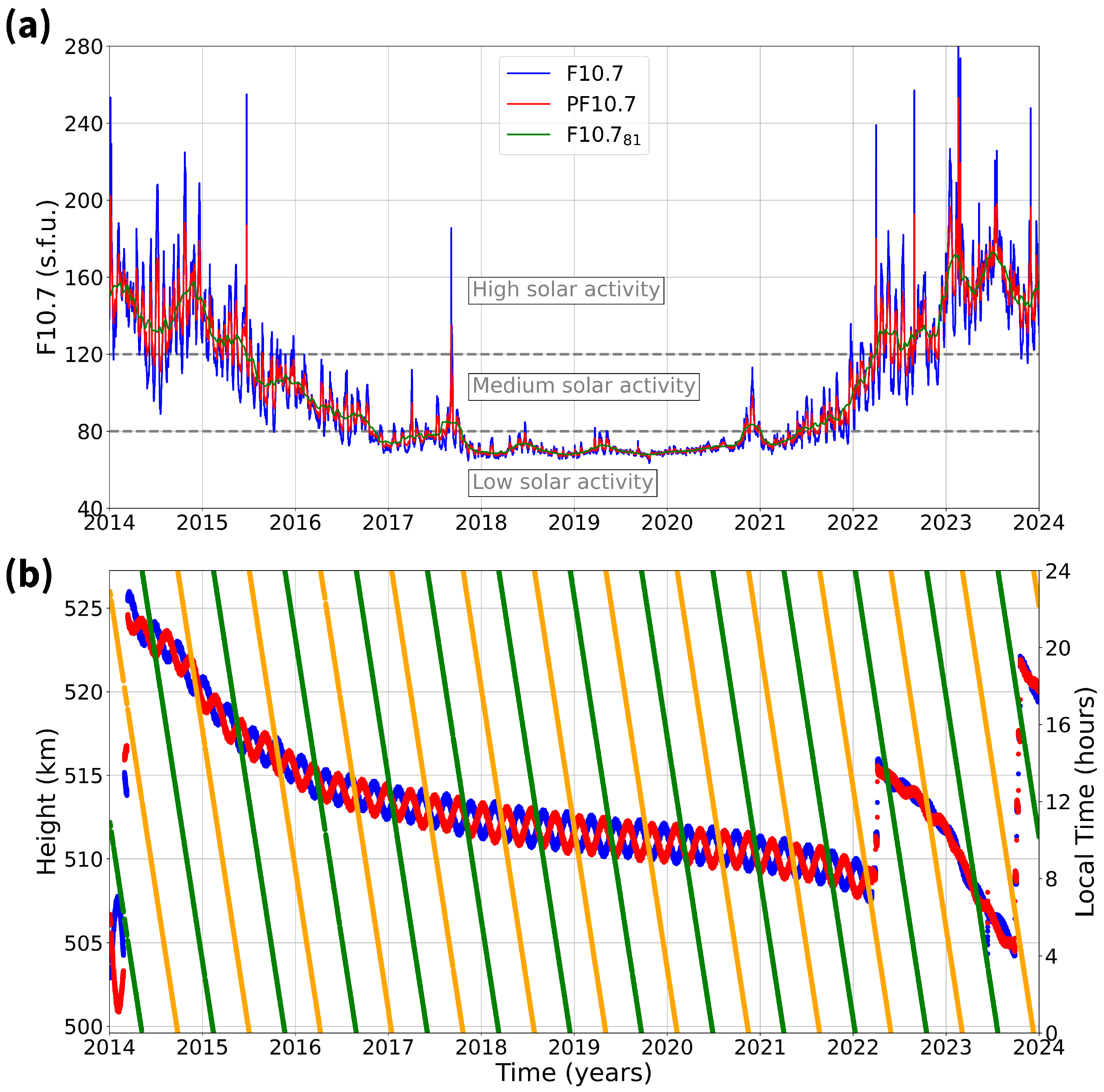
3.1. Swarm B Satellite In Situ Observations and Data Sorting

The ESA Swarm mission, launched at the end of 2013 and still in operation, consists of a trio of LEO satellites designed to investigate various aspects of the Earth’s magnetic field, magnetosphere, ionosphere, and upper atmosphere dynamics [34]. Swarm satellites, denoted as A, B, and C, share identical design and instrumentation, and orbit at LEO altitudes in near-polar circular orbits. Specifically, Swarm A and C share the same orbit configuration with an inclination of 87.35° and an east–west separation of 1°–1.5° in longitude, at an initial altitude of about 460 km from the ground. Meanwhile, Swarm B has an orbit inclination of 87.75°, at an initial altitude of about 510 km from the ground. The Swarm satellites drift in local time (LT) and cover a full LT cycle in approximately 130–140 days. This study focuses on the Swarm B satellite, by considering in situ T_e observations collected from 1 January 2014 to 31 December 2023, thus covering a full solar cycle (Figure 1a). In this timeframe, Swarm B’s altitude ranged between 500 and 530 km and covered different LTs, as reported in Figure 1b. In 2022 and 2023, Swarm B underwent two orbital altitude raises through maneuvers. Only the Swarm B observations from |30°| QD geomagnetic latitude ([35]) to the geomagnetic poles, for both hemispheres, were considered in this study.

Among the suite of Swarm instruments, here, we are interested in LPs that are included in the Electric Field Instrument (EFI) payload [36]. LPs provide in situ measurements of both N_e and T_e, with a sampling frequency of 2 Hz in harmonic mode. This is a level 1b product (EFIx_LP_1B), which regularly undergoes upgrades leading to continuous improvements in the data quality, which are classified through different product baselines identified by two digits in the EFIx_LP_1B filename [37]. For this study, we used the baseline 06, which includes the Lomidze et al. [38] correction factors in the EFIx_LP_1B files, and it is now considered the reference product. The nominal LP observations, recorded in high-gain (HG) mode, have been selected through data flags application [39]. Specifically, we selected those with Flags_LP = 1, Flags_Ne = (10,19,20), and Flags_Te = (10,19,20). Especially during periods of high solar activity, data quality is very often flagged as non-nominal in the equatorial region, probably due to problems with the current saturations of the Langmuir probes. This causes a significant reduction in the statistics in a latitude belt around the equator and gives us a further strong reason to focus our study on mid- and high latitudes, i.e., only the T_e observations above |30°| QD geomagnetic latitude, for both hemispheres, have been considered.

Lomidze et al. [38] devised a correction method for the Swarm LP data for both N_e and T_e. This correction is based on comparisons with measurements from ISRs, COSMIC/FORMOSAT-3 GPS radio occultations, and ionosondes. Pignalberi et al. [19] deeply investigated the effectiveness of the Lomidze et al. [38] correction to the Swarm T_e values, comparing them with IRI-modeled data and ISRs-measured values. The application of the correction improved the agreement between the Swarm-measured and IRI-modeled T_e values, by reducing the mean of residuals by 400 K on average. The improvement was confirmed through a comparison with the Jicamarca, Arecibo, and Millstone Hill ISRs observations. At the same time, Pignalberi et al. [19] evidenced how the calibration procedure is particularly effective at mid-latitudes and in the dayside sector due to the dataset used by Lomidze et al. [38] for the calibration parameter estimations. While the accuracy of the Swarm T_e observations would benefit from the inclusion of the latitudinal and diurnal dependence in the calibration procedure, the Lomidze et al. [38]-calibrated T_e dataset is the most reliable among the released datasets. Based on this and on the results by Pignalberi et al. [19], in this study, we used the Swarm B T_e measurements calibrated according to Lomidze et al. [38].

For the T_e data correction, Lomidze et al. [38] distinguished between measurements obtained in the HG and low-gain (LG) modes, which showed different features and calibration parameters. Since only the HG data are considered in this study, Equation (5) from Lomidze et al. [38] has been applied to the Swarm B T_e measurements for data correction, which is reported below for reference:

$$T_{\mathrm{e},\mathrm{L}\mathrm{o}\mathrm{m}}=1.2248\cdot T_{\mathrm{e},\mathrm{L}\mathrm{P}}-1047+8.548\cdot N_{\mathrm{e},\mathrm{L}\mathrm{P}}/{10}^4.$$

(1)

In Equation (1), $T_{\mathrm{e},\mathrm{L}\mathrm{P}}$ and $N_{\mathrm{e},\mathrm{L}\mathrm{P}}$ are electron temperature and density, respectively, measured with Swarm B LPs, while $T_{\mathrm{e},\mathrm{L}\mathrm{o}\mathrm{m}}$ are electron temperature values after the application of the Lomidze et al. [38] correction. The T_e values are in K, while the N_e values are in cm⁻³.

The Swarm LP data are freely accessible for download at https://swarm-diss.eo.esa.int/, accessed on 15 April 2024.

In addition to the filtering based on LP’s flags, we implemented other constraints to keep the focus on the large-scale climatological features of T_e. In particular, we restricted the T_e magnitude within the range of 100 K and 10,000 K and considered only magnetically quiet time periods for which the global geomagnetic index Kp ≤ 3. Three-hourly values of the Kp geomagnetic activity index were downloaded from the OMNIWeb Data Explorer website https://omniweb.gsfc.nasa.gov/form/dx1.html, accessed on 15 April 2024. The filtering based on the Kp index is driven by the motivation of this study, for which the representation of the geomagnetic activity influence on T_e is out of the study scope. Differently, the need to limit the upper range of T_e at 10,000 K is motivated by the Pignalberi et al. [40] study which showed that around specific MLTs, particularly at low and mid-latitudes, Swarm LP data are characterized by characteristic trains of T_e spikes. These spikes are associated with instrumental issues not captured by LP flags and have to be considered outliers. The same study also identified very high T_e values (≥6000 K) at high latitudes, but these show well-defined spatial and time variations associated with physical phenomena characterizing the high-latitude ionosphere, and then they can be considered trustworthy. The upper threshold at 10,000 K is a tradeoff to limit the influence of T_e spikes identified by [40], while allowing the representation of high T_e values at high latitudes.

To properly characterize the T_e variations with solar activity, the spatial, local time, and seasonal variations have to be specified. Indeed, T_e variations with solar activity and season can be considered second-order effects when compared to the variations with latitude, altitude, and local time, which are first-order effects [15]. The altitudinal variation is inherently constrained by the Swarm B orbit (Figure 1b). Instead, the latitudinal, local time, and seasonal variations have to be extracted by sorting the Swarm B T_e observations. Since the data used in this study concern the topside ionosphere, we use geomagnetic coordinates, specifically, QD geomagnetic latitude [35] and magnetic local time (MLT). Indeed, plasma dynamics in the topside ionosphere is mainly driven by the plasma ambipolar diffusion along geomagnetic field lines [5,6], which makes the use of geomagnetic coordinates the natural basis to represent plasma variations at these altitudes.

First, the data were sorted into three seasons around solstices and combined equinoxes:

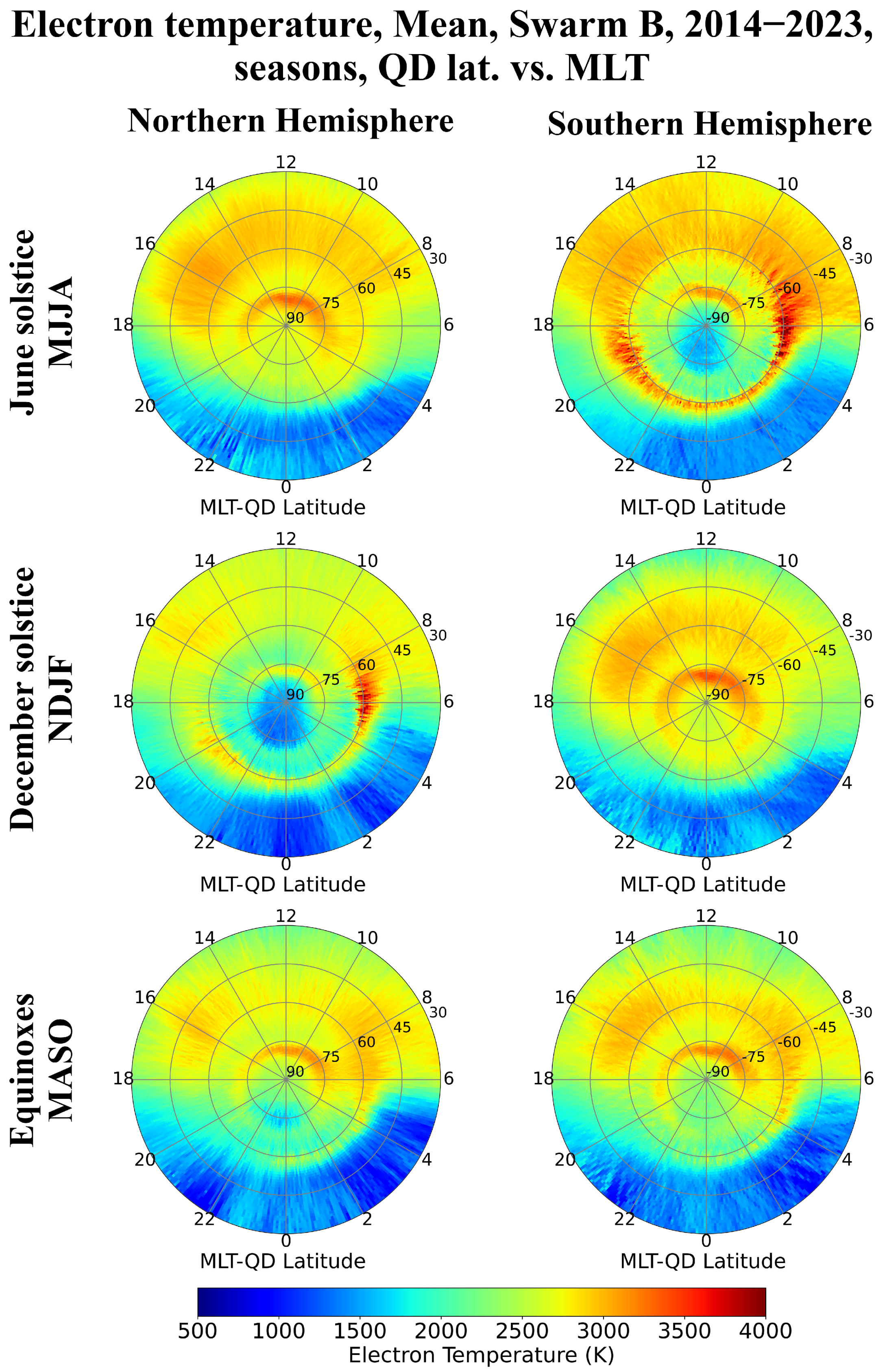
• June solstice: the months of May, June, July, and August. The summer season in the Northern Hemisphere, and the winter season in the Southern Hemisphere;
• December solstice: the months of November, December, January, and February. The winter season in the Northern Hemisphere, and the summer season in the Southern Hemisphere;
• Equinoxes: the months of March, April, September, and October. Equinoctial seasons in both hemispheres.

The equinoctial data have been merged based on the results by [19], and a preliminary analysis which evidenced marginal differences between equinoxes. Longitudinal variations in geomagnetic coordinates have not been considered, being a third-order effect characterizing the T_e ionospheric variations [15].

Subsequently, for each season, the data were sorted as a function of the QD latitude and MLT with the following binning:

• QD latitude: from |30°| to |90°| in steps of 1°, for both hemispheres, 120 bins in total;
• MLT: from 00:00 to 24:00 in steps of 4 min, 360 bins in total.

For each bin, we calculated the mean T_e value after removing the outliers through the median absolute deviation filtering procedure as described in Section 3.3 of [41]. Figure 2 shows polar maps, in MLT vs. QD latitude, of the mean T_e from the Swarm B LP observations, as a function of the season and for both hemispheres. Latitudinal, LT, and seasonal T_e variations were carefully described in the previous study by Pignalberi et al. [19] and will be only briefly outlined here. Instead, since this study focuses on the T_e variations with solar activity, maps in Figure 2 serve as a reference to highlight how the different solar activity levels possibly change both the magnitude and the spatial and time features of T_e.

From Figure 2, T_e shows a diurnal trend that changes with latitude and season. Mid-latitudes (|30°|–|50°| QD latitude) exhibit a well-defined diurnal pattern with high T_e at dayside and low T_e at nightside, consistent with the solar EUV radiation diurnal pattern. Differently, high latitudes show a more complex diurnal variation, which is also strongly dependent on season, with localized regions of enhanced T_e. In particular, the highest T_e characterizes the nightside and morning sectors of the mid-latitude ionospheric trough at sub-auroral latitudes (|55°|–|65°| QD latitude, [42]) in the local winter season, and the dayside sector in the polar cusp region (|70°|–|80°| QD latitude), especially in the local summer season. These patterns are consistent with the heating associated with the particle’s precipitation and the coupling between the plasmasphere, magnetosphere, and ionosphere [43,44,45,46], and will be discussed in Section 5. For further details, the reader may refer to [19].

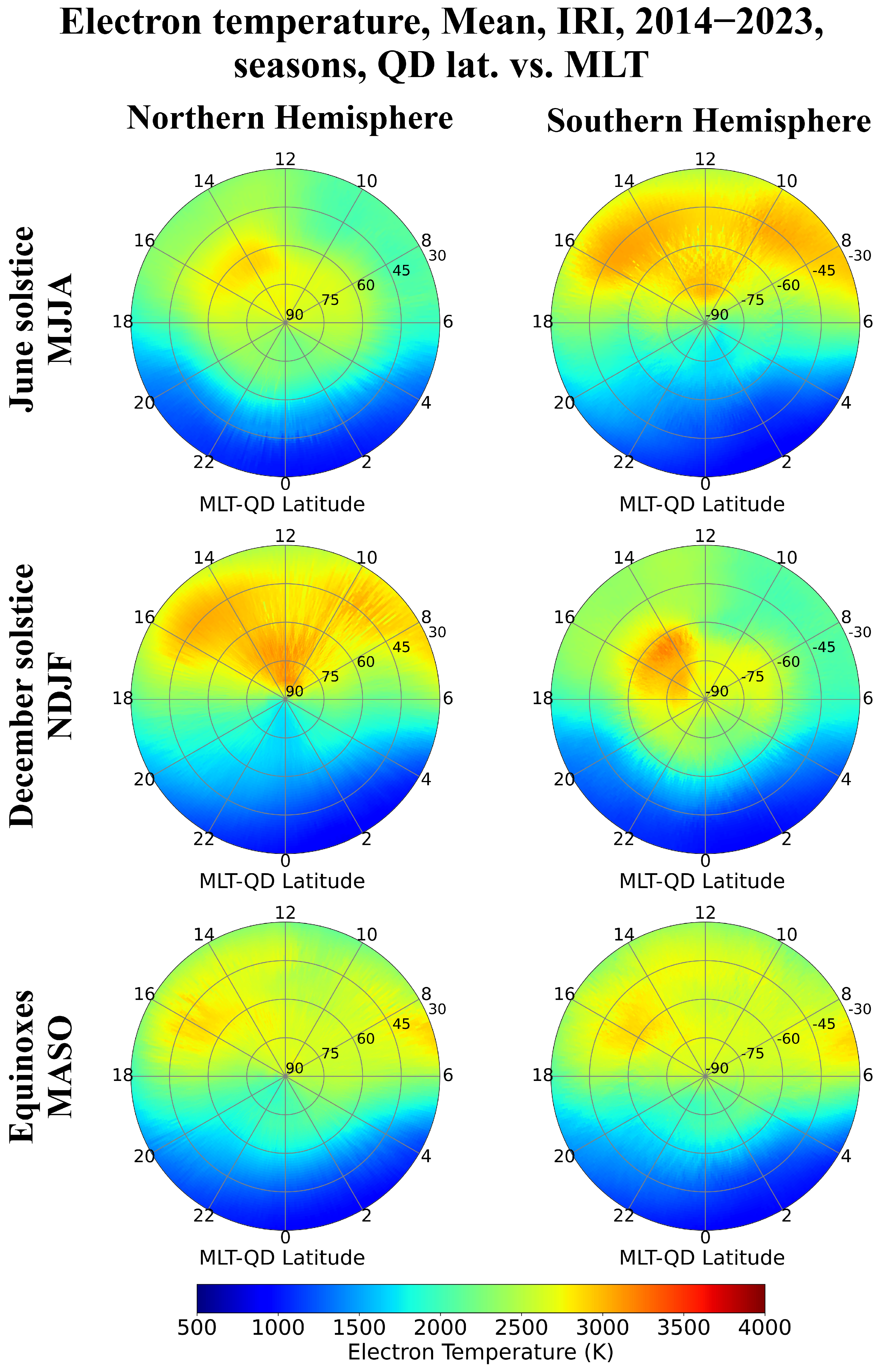
3.2. Electron Temperature Modeling by IRI

IRI is an empirical climatological ionospheric model relying on ground-based and space-based observations of the ionosphere collected over the recent decades on a global scale ([16] and references therein). The IRI project was initiated in 1968 and sponsored by the Committee on Space Research (COSPAR) and the International Union of Radio Science (URSI). As of April 2014, IRI has become the official International Standardization Organization (ISO) standard for the ionosphere [47].

The last version of IRI, i.e., IRI-2020 [16], includes two options to model T_e based on the former Bil-1995 model and the newer TBT-2012 model. The Bil-1995 model is based on the Brace and Theis [14] and Spenner and Pluge [13] models, which were included in IRI through the works of Bilitza [48] and Bilitza et al. [49]. Meanwhile, the TBT-2012 model is based on the works by Truhlik et al. [17,18], which was then upgraded also by including the solar activity variation [15], based on the achievements of Truhlik et al. [32]. The inclusion of the solar activity variation defines the TBT-2012+SA model [15], which is the IRI-2020 default option for T_e modeling, and is the model used in this study.

The TBT-2012+SA model is based on a large compilation of T_e satellite observations, as described in [12,31], which allowed for the description of T_e in a range of altitudes between 60 km and 2000 km from the ground. Specifically, TBT-2012+SA models T_e at five fixed anchor points at 350, 550, 850, 1400, and 2000 km of altitude through a spherical harmonic expansion in a system of associated Legendre polynomials, as a function of MLT and invdip [15]. Invdip is a latitude coordinate based on a combination of invariant and dip latitudes [18]. Spherical harmonic coefficients were calculated independently of the hemisphere for the summer and winter solstices and for the combined equinoxes. Consequently, possible interhemispheric differences are not considered by the model.

On top of the latitudinal, MLT, and seasonal variations at a fixed altitude, Truhlik et al. [15] introduced the solar activity variation by adding to the core T_e model a correction term that is a function of the PF10.7 solar activity proxy. PF10.7 [50] is the average between the daily F10.7 solar activity index [51] and its 81-day running mean (F10.7₈₁). PF10.7 has shown a higher correlation with the EUV flux and, thus, provides the best description of the corresponding solar activity variation in ionospheric parameters [52]. The solar activity correction term is a function depending upon MLT and invdip, for each season and altitude anchor point and is based on the results by Bilitza et al. [31] and Truhlik et al. [32]. Specifically, the solar activity function includes a daytime (13:00 ± 02:30 MLT) and nighttime (01:00 ± 03:00 MLT) dependence, for three levels of solar activity, respectively for PF10.7 < 110 sfu (solar flux units; low solar activity), 110 ≤ PF10.7 ≤ 180 sfu (medium solar activity), and PF10.7 > 180 sfu (high solar activity). The solar activity function is quadratic between 110 sfu and 180 sfu, and linear outside this range. For full details on the TBT-2012+SA model, the reader may refer to [15].

After modeling T_e at five anchor points at 350, 550, 850, 1400, and 2000 km of altitude, IRI builds the complete vertical T_e profile through the application of a Booker profile [53], as described in the Appendix sections of [16,54]. This approach also resulted in the creation of a better model of T_i, recently included in IRI-2020 [55].

IRI-2020 with the TBT-2012+SA option was run along each Swarm B satellite orbit, with the same time and spatial resolution of LPs observations, for the whole dataset (see Section 3.1). In this way, a one-to-one comparison between the measured and modeled T_e values is guaranteed. The IRI-2020 Fortran code is available on the IRI website (http://irimodel.org/, accessed on 15 April 2024).

The IRI-modeled T_e values underwent the same binning procedure as the Swarm B observations, as described in Section 3.1. Corresponding polar maps of IRI-modeled mean T_e values are shown in Figure 3, with the same layout and color scale as Figure 2.

Compared to the Swarm B T_e observations (Figure 2), the IRI-modeled T_e values show less complex diurnal and latitudinal patterns at high latitudes, while they describe trends similar to the Swarm B observations at mid-latitudes. According to [19], differences between observations and models at high latitudes come from the limited spatial and time resolutions of the TBT-2012+SA model. The current model resolution does not allow for the proper description of the very steep and localized T_e enhancements at the polar cusp and sub-auroral boundaries. Moreover, the IRI-modeled T_e shows a consistent seasonal variation at mid-latitudes in the dayside sector with the highest values in the local winter, while Swarm B shows a less marked seasonal difference for those conditions. This can be due to some underestimation of the TBT-2012+SA model in summer and overestimation in winter at mid-latitudes, as seen in Figure 6 of [19].

3.3. Millstone Hill Incoherent Scatter Radar Remote Sensing Observations

ISRs are ground-based facilities that utilize the Thomson backscatter from electrons in the ionosphere to retrieve various ionospheric parameters, including T_e, from about 100 to 1000 km from the ground [56].

In this study, we used the Millstone Hill ISR T_e observations for validation purposes. Millstone Hill is located at mid-geographic latitudes (42.6° N, 71.5° W; USA), but is a mid-latitude/sub-auroral station when considering geomagnetic coordinates. Indeed, it has a QD latitude of 51.8° N. Since the comparison with ISR is statistical, we considered data recorded from 1976 to 2020. Therefore, although ISR data are not continuously available, the dataset provides a sufficiently uniform representation of diurnal and seasonal trends, for different solar activity levels. For a proper comparison with Swarm B observations, we selected ISR T_e observations recorded within the range of 510 ± 20 km.

The Millstone Hill ISR data were obtained from the website http://cedar.openmadrigal.org, accessed on 15 April 2024.

4. Results

The Swarm B dataset covers the years from the beginning of 2014 to the end of 2023, i.e., from the maximum of the 24th solar cycle to the upcoming maximum of the 25th solar cycle, as depicted in Figure 1a. In this timeframe, the PF10.7 solar activity proxy ranged between 65 sfu and 253 sfu, with the F10.7₈₁ between 68 sfu and 175 sfu. Compared to previous solar cycles, this one was rather weak. This affected the choice of the solar activity level thresholds used to sort the data as a function of solar activity. The data were sorted in three solar activity bins as a function of PF10.7:

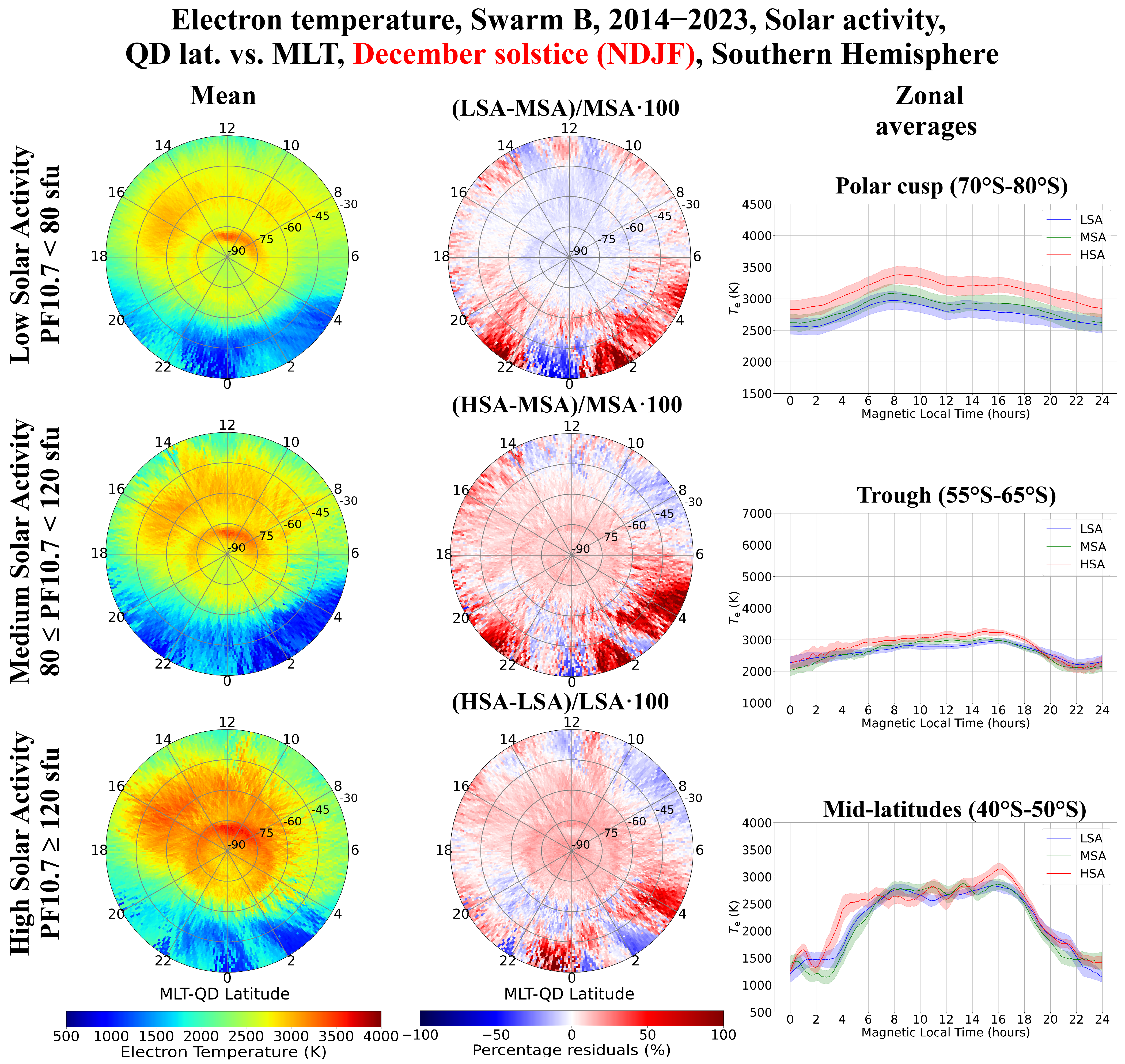
• Low solar activity (LSA): PF10.7 < 80 sfu;
• Medium solar activity (MSA): 80 ≤ PF10.7 < 120 sfu;
• High solar activity (HSA): PF10.7 ≥ 120 sfu.

It is worth noting that during the Swarm B lifetime, the high-solar-activity conditions selected by [15], i.e., PF10.7 > 180 sfu, were reached only occasionally. As a consequence, the available dataset does not cover the entire spectrum of solar activity conditions described by the IRI-2020 TBT-2012+SA model. Daily values of the F10.7 solar activity index were downloaded from the OMNIWeb Data Explorer website https://omniweb.gsfc.nasa.gov/form/dx1.html, accessed on 15 April 2024.

For each of the three solar activity levels, both measured and modeled T_e values were sorted as a function of season, QD latitude, and MLT, as described in Section 3.1, and polar maps such as Figure 2 and Figure 3 were calculated for both hemispheres. In the next section, for brevity, the paper shows results for the Southern Hemisphere, as the overall trends and observations are similar among the two hemispheres. The results for the Northern Hemisphere are provided in the Supplementary Materials.

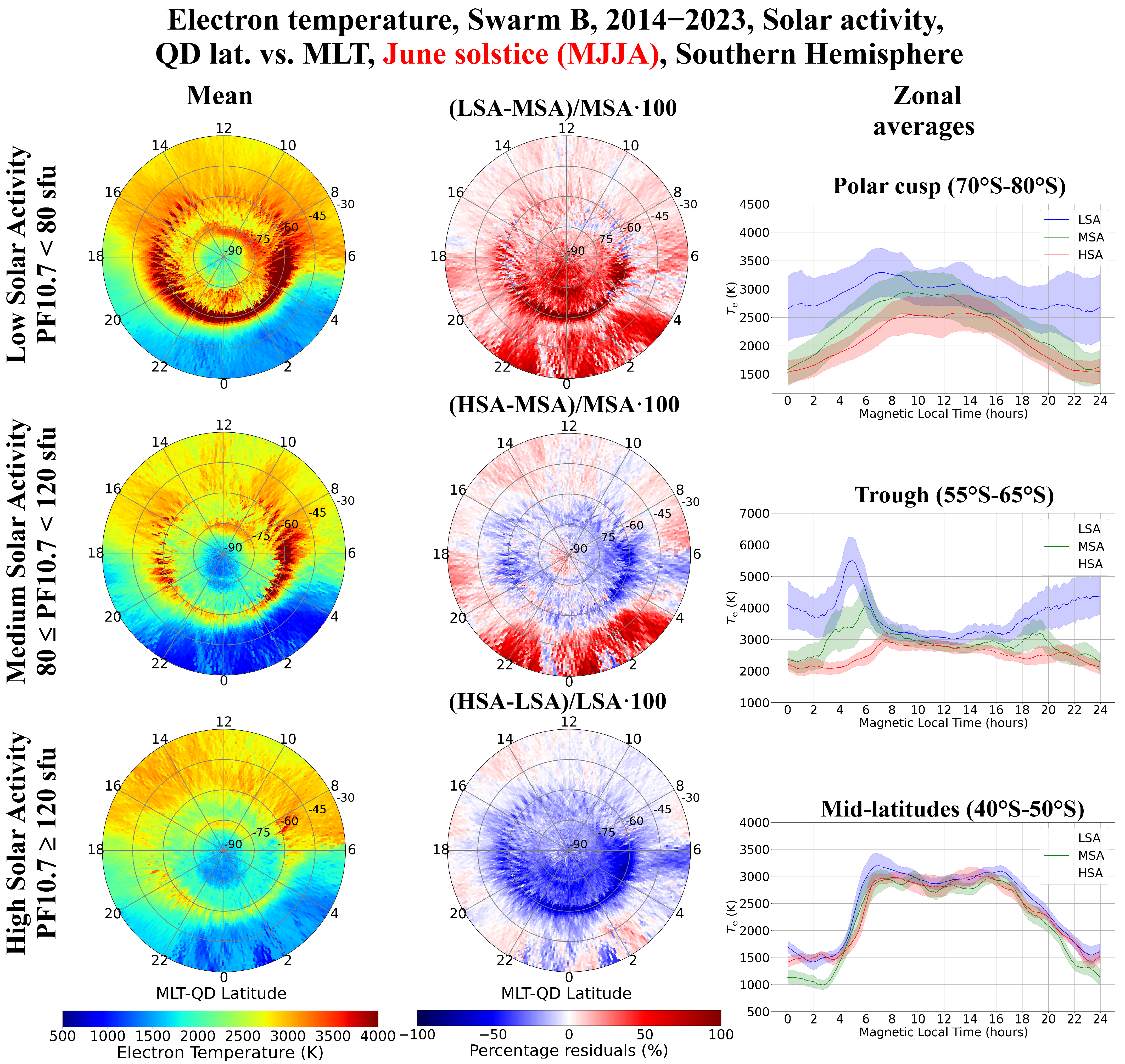
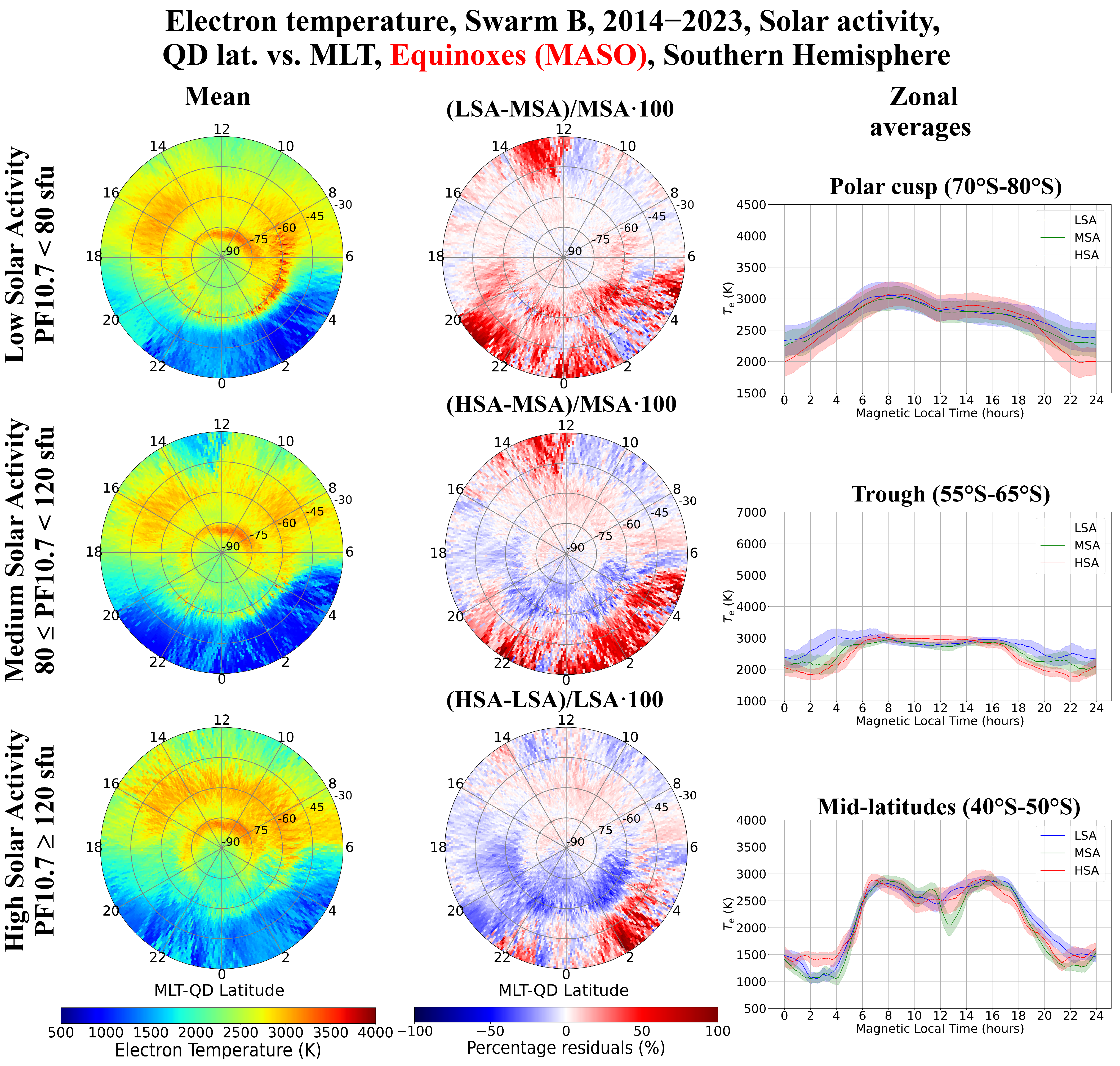
4.1. Solar Activity Variation as Described by Swarm B Observations

Figure 4, Figure 5 and Figure 6 show how the solar activity variations affect Swarm B observations in the Southern Hemisphere for the December solstice, June solstice, and equinoxes, respectively. Corresponding plots for the Northern Hemisphere are in Figures S1–S3 in the Supplementary Materials. The first column of each figure shows the polar maps, in MLT vs. QD latitude, of the mean T_e as a function of solar activity level. We also calculated the percentage residuals of these mean values for different solar activity levels:

$$T_{\mathrm{e},\mathrm{L}\mathrm{S}\mathrm{A}-\mathrm{M}\mathrm{S}\mathrm{A}} [\%]=\frac{T_{\mathrm{e},\mathrm{L}\mathrm{S}\mathrm{A}}-T_{\mathrm{e},\mathrm{M}\mathrm{S}\mathrm{A}} }{T_{\mathrm{e},\mathrm{M}\mathrm{S}\mathrm{A}} }\times 100,$$

(2)

$$T_{\mathrm{e},\mathrm{H}\mathrm{S}\mathrm{A}-\mathrm{M}\mathrm{S}\mathrm{A}} [\%]=\frac{T_{\mathrm{e},\mathrm{H}\mathrm{S}\mathrm{A}}-T_{\mathrm{e},\mathrm{M}\mathrm{S}\mathrm{A}} }{T_{\mathrm{e},\mathrm{M}\mathrm{S}\mathrm{A}} }\times 100,$$

(3)

$$T_{\mathrm{e},\mathrm{H}\mathrm{S}\mathrm{A}-\mathrm{L}\mathrm{S}\mathrm{A}} [\%]=\frac{T_{\mathrm{e},\mathrm{H}\mathrm{S}\mathrm{A}}-T_{\mathrm{e},\mathrm{L}\mathrm{S}\mathrm{A}} }{T_{\mathrm{e},\mathrm{L}\mathrm{S}\mathrm{A}} }\times 100.$$

(4)

Corresponding polar maps of percentage residuals are shown in the second column plots of Figure 4, Figure 5, Figure 6 and Figures S1–S3. In these plots, the red color indicates values higher than those recorded for the reference solar activity level (the denominator in Equations (2)–(4)), while the blue color is for values lower than those recorded for the reference.

The third column plots in Figure 4, Figure 5 and Figure 6 show the T_e diurnal variations for the selected ranges of latitudes: for the three different solar activity levels considered. We selected three ranges of latitudes as representative of the polar cusp region (QD latitudes between |70°| and |80°|), mid-latitude ionospheric trough (QD latitudes between |55°| and |65°|), and mid-latitudes (QD latitudes between |40°| and |50°|). Starting from the mean values shown on the first-column maps, for each of these ranges, we calculated the latitudinal average and corresponding standard deviation, as a function of MLT. Latitudinal, i.e., zonal, average values are represented by solid lines, while standard deviations are represented by shaded areas.

A first look at Figure 4, Figure 5 and Figure 6 highlights that the T_e variations with solar activity levels are strongly dependent on season, QD latitude, and MLT, as highlighted by previous studies. In a nutshell, it is not possible to identify a simple increasing or decreasing trend with solar activity level, which can be valid for all the geophysical conditions studied here. The largest T_e variations with solar activity characterize the high latitudes in the local winter season, i.e., the June solstice season in the Southern Hemisphere (Figure 5). Moreover, the trends with solar activity levels at high latitudes are also reversed between the local summer (Figure 4) and the local winter (Figure 5). Differently, equinoxes show a T_e variation with solar activity which is negligible for most of the conditions (Figure 6).

An increasing trend with solar activity characterizes the polar cusp and trough latitudes in summer (Figure 4), with T_e,HSA ≥ T_e,MSA ≥ T_e,LSA for most MLTs, particularly at polar cusp latitudes. Differently, mid-latitudes do not show a clear trend with solar activity irrespective of season. Instead, a decreasing trend with solar activity characterizes the polar cusp and trough latitudes in winter (Figure 5), with T_e,HSA ≤ T_e,MSA ≤ T_e,LSA for most MLTs but particularly in the nightside sector. However, the increasing T_e trend in summer and the decreasing trend in winter show very different relative magnitudes. Indeed, while for the summer season, the increasing trend is at most about |30%|, for different solar activity levels at high latitudes (Figure 4), the decreasing trend in the winter season can reach up to |100%| from MSA to LSA in the nightside trough (Figure 5). The latter is by far the largest T_e variation with solar activity level from the Swarm B observations, and it is statistically robust when considering the dispersion of data highlighted in the third-column panels.

A completely different picture characterizes the equinoxes (Figure 6), where most of the T_e variations with solar activity are inside the dispersion of data and the largest percentage residual values are at mid-latitudes, particularly in the nightside.

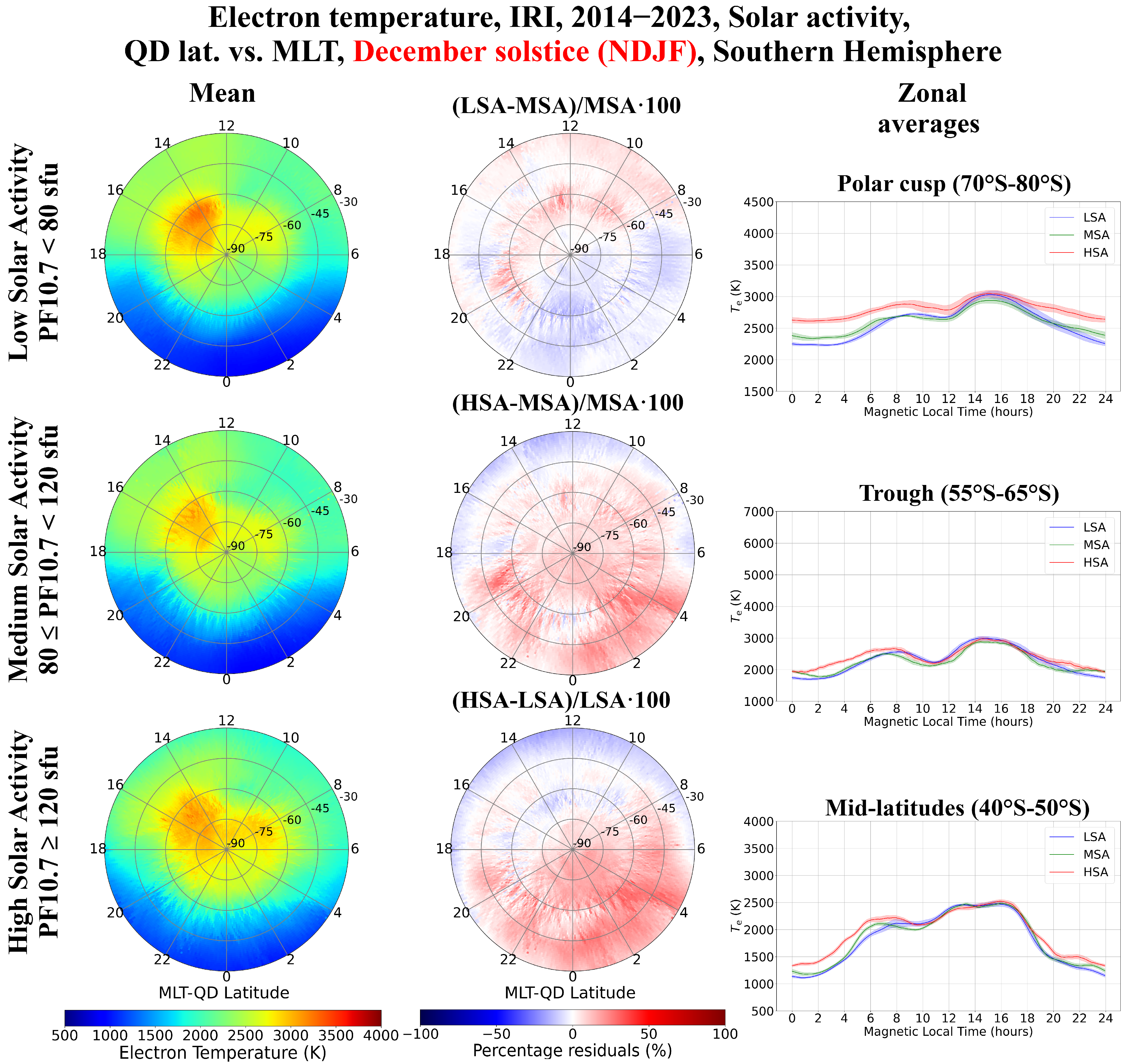
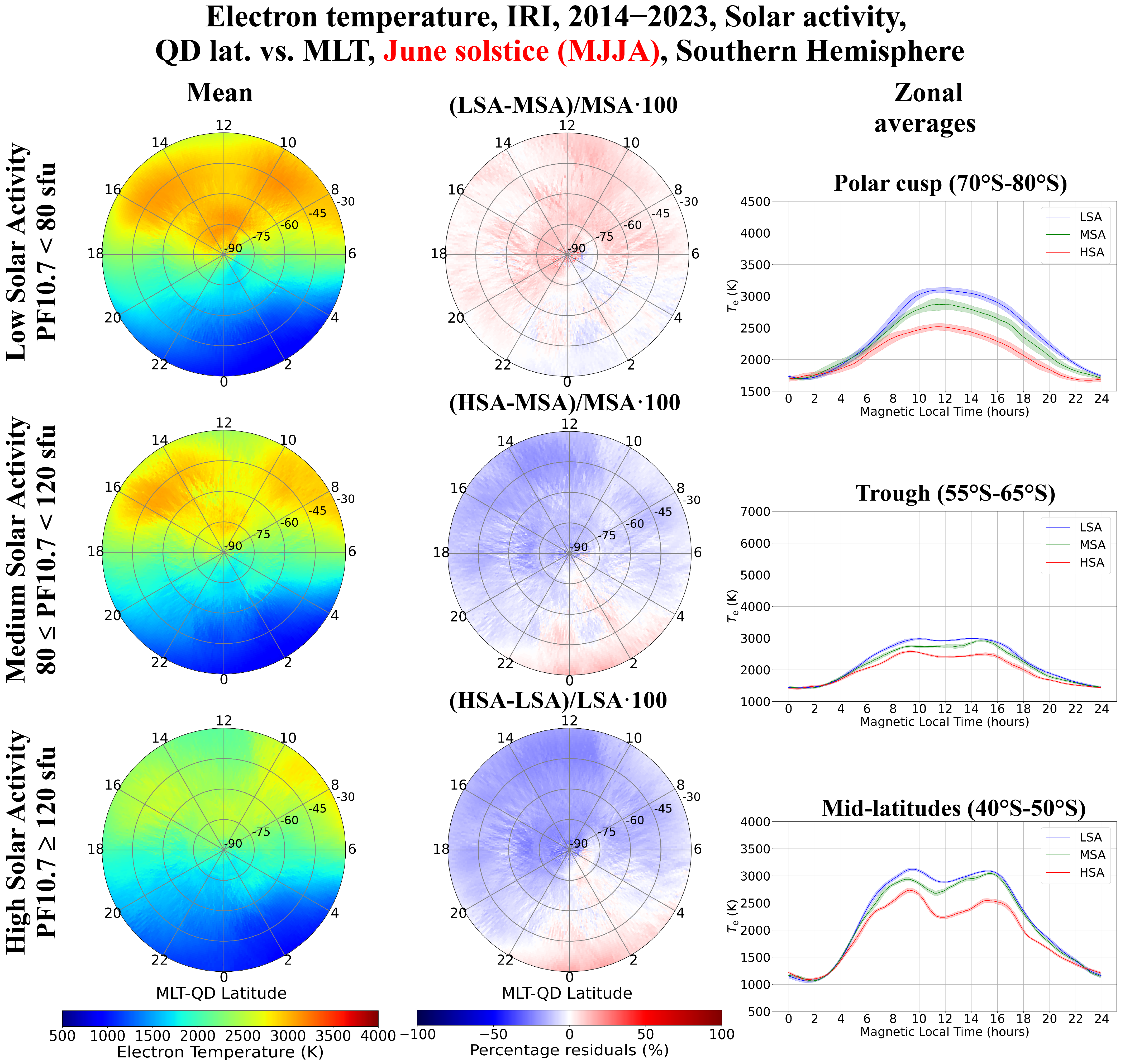
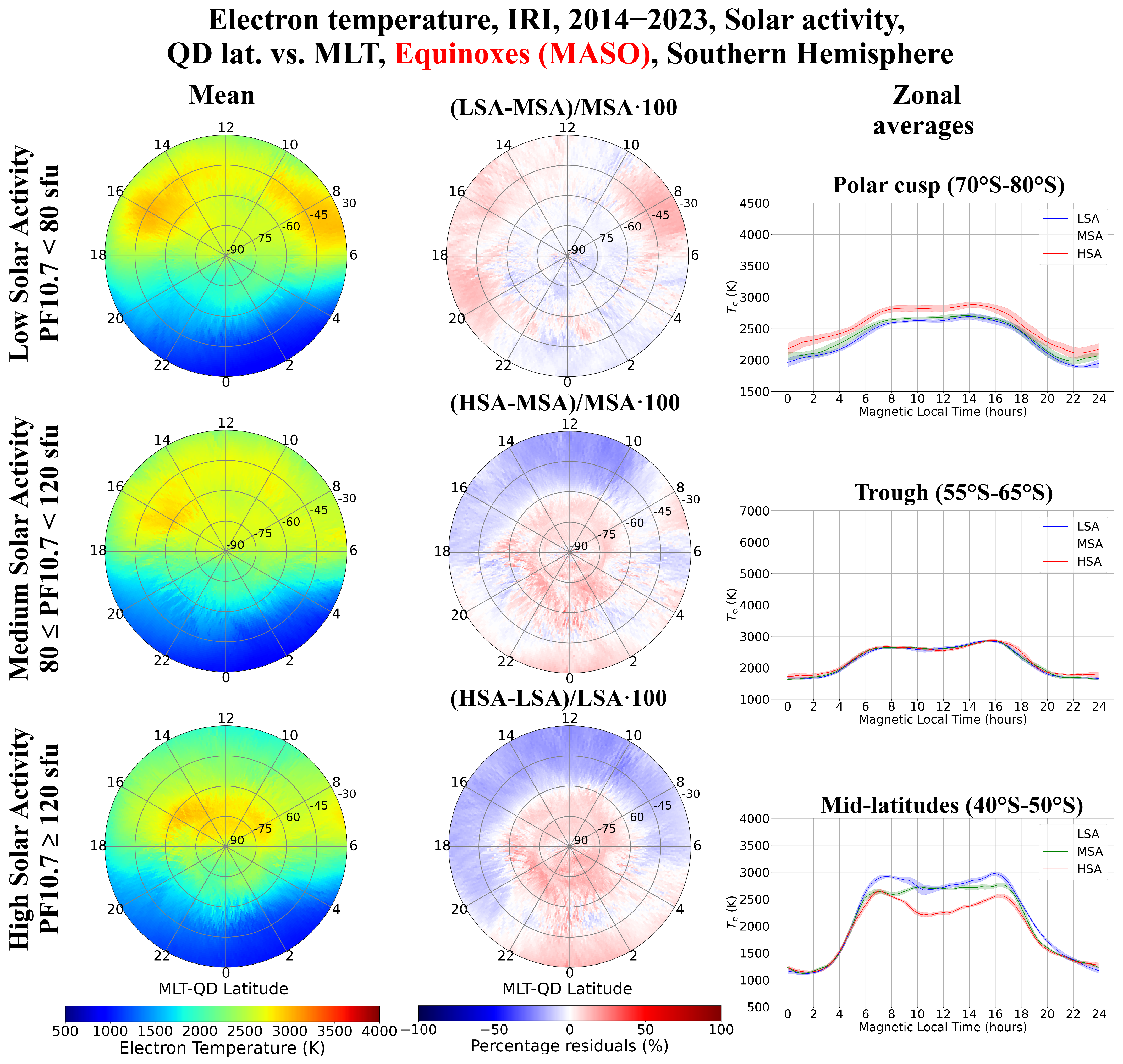
4.2. Solar Activity Variation as Described by the IRI Model

Since the IRI-2020 dataset has a one-to-one correspondence with the Swarm B dataset (see Section 3.2), the same statistical analysis shown in Section 4.1 has been repeated here for the IRI model. Figure 7, Figure 8 and Figure 9 show how the solar activity variations affect the T_e values modeled by IRI-2020 using the TBT-2012+SA option at the Southern Hemisphere for the December solstice, June solstice, and equinoxes, respectively. Corresponding plots for the Northern Hemisphere are in Figures S4–S6 in the Supplementary Materials.

In the description of IRI-modeled results we have to remember that, as already highlighted in Section 3.2, the TBT-2012+SA model does not reproduce all the high-latitude features seen by Swarm B.

Figure 7, Figure 8 and Figure 9 highlight interesting T_e variations as a function of solar activity. Compared to the observations, the modeled values show smoother spatial and diurnal patterns, with a relatively small dispersion around zonal mean values. Similar to the observations, the IRI-modeled values also show a decreasing trend with solar activity in the local winter (Figure 8), with T_e,HSA ≤ T_e,MSA ≤ T_e,LSA at both mid- and high latitudes. Interestingly, the decreasing T_e trend is restricted to the dayside, while negligible differences are observed on the nightside, this trend being shared among different latitudes. The increasing trend with solar activity for the summer season is described by modeled values above all at polar cusp latitudes and on the nightside at different latitudes (Figure 7), with T_e,HSA ≥ T_e,MSA ≥ T_e,LSA. Similarly to the observations, the modeled values also show the largest variations with solar activity in winter, although with different diurnal patterns at high latitudes. Equinoxes (Figure 9) show a more complex picture with an increasing T_e with solar activity at polar cusp latitudes, no solar activity variation at the trough, and a decreasing T_e with solar activity at mid-latitudes on the dayside.

To further compare IRI-modeled values with Swarm B observations, we calculated the ratios between the modeled and measured T_e values:

$$\mathrm{R}\mathrm{a}\mathrm{t}\mathrm{i}\mathrm{o}=\frac{\mathrm{M}\mathrm{o}\mathrm{d}\mathrm{e}\mathrm{l}\mathrm{e}\mathrm{d} T_{\mathrm{e}}}{\mathrm{M}\mathrm{e}\mathrm{a}\mathrm{s}\mathrm{u}\mathrm{r}\mathrm{e}\mathrm{d} T_{\mathrm{e}}}.$$

(5)

Ratio values allow for the proper comparison of T_e values collected under different geophysical conditions, i.e., QD latitude, MLT, season, and solar activity level. A perfect model should provide ratio values equal to unity, irrespective of the different geophysical conditions. If so, the model would be able to properly describe all the variations embedded in the observations. The ratio in excess of unity indicates an overestimation on the part of the model, while the ratio below unity indicates an underestimation on the part of the model.

Figure 10 summarizes the results obtained from ratios calculated through Equation (5) for the whole dataset. In panel (a), ratios between the modeled and measured T_e values are binned as a function of the PF10.7 solar activity proxy. Panel (b) shows the probability density histogram of ratio values, with corresponding statistical metrics, for the entire dataset. Panel c) shows the probability density histograms of ratio values as a function of solar activity. The analysis based on ratios confirms the overall underestimation of the IRI-modeled values when compared to the Swarm B observations, in agreement with Pignalberi et al.’s [19] results, with a mean ratio equal to 0.914 and a median ratio equal to 0.892. The difference between the mean and median ratio is mainly caused by the slight asymmetric distribution of the ratios, which shows a longer tail at the lowest ratio values where it departs from a Gaussian distribution, which is to be mainly attributed to LSA as evidenced by Figure 10c. The standard deviation and IQR dispersion parameters are instead very similar: 0.301 vs. 0.305.

Figure 10a,c suggest that the IRI underestimation is a feature shared across the solar activity levels of our dataset. The absence of any trend in ratios points out that overall, the IRI model correctly describes the variation associated with solar activity level. The largest IRI underestimation is found for very low solar activity (65–80 sfu) where median values reach 0.85, while it is around 0.90 for higher solar activity.

Overall, the statistics of Figure 10 confirm that IRI-2020 correctly describes the T_e solar activity variation through the TBT-2012+SA model, although with an overall underestimation of about 10%. From Figure 4, Figure 5, Figure 6, Figure 7, Figure 8 and Figure 9, the largest underestimation made by IRI has to be ascribed to the different description of high latitudes, particularly at polar cusp and trough regions, where IRI shows the largest departures from the observations.

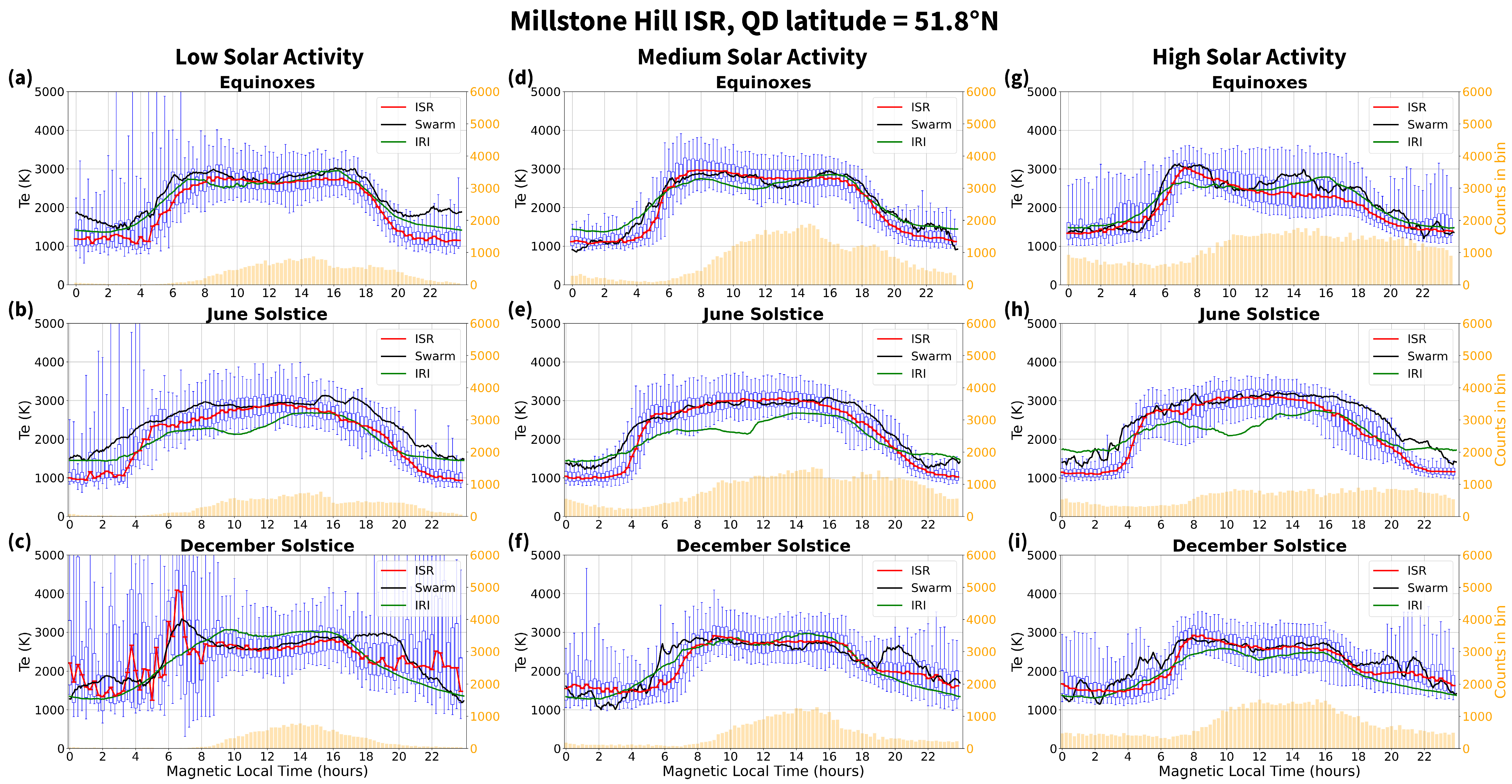
4.3. Comparison against Millstone Hill Incoherent Scatter Radar Observations

Since the ISR observations are considered the reference for the study of ionospheric plasma parameters, Pignalberi et al. [19] performed a statistical comparison among T_e values measured by Swarm satellites, modeled by IRI, and measured by the Jicamarca, Arecibo, and Millstone Hill ISRs. That study did not investigate the T_e variations with solar activity; therefore, we now extend that comparison by sorting out the solar activity level. Among the three ISRs, only Millstone Hill is inside the QD latitude range selected for this study, being also one of the few ISRs at mid- and high latitudes providing a database wide enough to cover the different MLTs, seasons, and solar activity levels at about 500 km of altitude. Consequently, our comparison is based on the Millstone Hill ISR observations only.

The T_e observations at 510 ± 20 km recorded by the Millstone Hill ISR were binned as a function of MLT, season, and solar activity. The T_e observations were first sorted as a function of PF10.7, by applying the same thresholds as before, with the only difference being that the HSA range has now been limited to a maximum of 200 sfu to be consistent with the Swarm B dataset, which is characterized by very few values recorded for PF10.7 > 200 sfu. Then, the same seasonal binning as before was applied, and for each season, the diurnal trend was described by binning data in fifteen-minute MLT-wide bins. For each of these bins, we calculated the following statistics: median, first quartile (i.e., the 25th percentile), third quartile (i.e., the 75th percentile), and the 5th and 95th percentiles. The results are provided in Figure 11 in a boxplot representation. Since the comparison is made on a statistical basis, the Swarm B and IRI-2020 median values at the Millstone Hill ISR QD latitude 51.8° N, have been calculated and overplotted to boxplots in Figure 11. It is worth noting that the Swarm B and IRI-2020 median values in Figure 11 were obtained without taking into account any longitudinal dependence. However, this should introduce only a small uncertainty considering that longitudinal variations in T_e are a third-order effect [15], especially in the topside ionosphere.

The agreement between the Swarm B and ISR observations is consistent across different solar activity levels considering the natural variability of T_e as shown by the dispersion parameters associated with ISR observations. The Swarm B observations correctly describe both the diurnal and seasonal variations at Millstone Hill’s latitude, for low, mid-, and high solar activity. The agreement is remarkable in the dayside sector, while the Swarm B observations show a tendency to slightly overestimate T_e in the nightside sector for the June solstice (summer season), especially for LSA. A similar behavior also affects equinoxes for LSA. IRI shows good agreement with the ISR observations for equinoxes and the December solstice (winter season), irrespective of solar activity level, while differences arise for the June solstice (summer season) for both the dayside and nightside sectors. Specifically, in summer and irrespective of solar activity, IRI shows an underestimation during the daytime and an overestimation during the nighttime. The ISR observations show the largest dispersion for LSA, particularly during the nighttime where very few observations are available in the selected dataset.

5. Discussion

5.1. Physical Processes Affecting the T_e Variations in the Ionosphere

For the interpretation and discussion of the results, it is important to mention the basic physical mechanisms concerning T_e in the ionosphere. The electron temperature results from several major physical processes that enter into the equation of the energy balance of electrons [57]: (a) heating by photoelectrons, which are produced mainly by solar EUV radiation and particle precipitation; (b) cooling during collisions with ambient ions and neutrals; and (c) divergence heat flux due to field-aligned conductivity.

As solar activity increases, all of these factors increase and, thus, depending on specific conditions, T_e may increase, decrease, or remain constant (e.g., [25]). This is drastically different from the behavior of N_e, which always increases with increasing solar activity (e.g., [26,31,58]). Thus, if we consider the monotonicity of N_e vs. PF10.7, we can also consider the whole problem as a variant of the dependence of T_e on N_e. However, the description of the T_e vs. N_e dependence is itself challenging (e.g., [59]), also involving problems of N_e data availability and accuracy, whereas obtaining data on solar activity (e.g., PF10.7 index) is a much simpler task. Furthermore, another obstacle in the description of the dependence of T_e on solar activity is that T_e does not exhibit large solar cycle changes [26], and these changes, if any, are often smaller than either the measurement error or the standard deviation (e.g., [60]), as follows from Figure 4, Figure 5 and Figure 6 (right panels), Figures S1–S3 (right panels), and Figure 11. The standard deviation is the result of both the measurement uncertainty, depending on both the instrument design and the measurement technique, and the natural variability of measurements in a given bin.

In order to interpret the high-latitude T_e structures, it must be borne in mind that electrons, of which temperature is a measure of energy, consist mainly of two populations [61]. The first one consists of thermal electrons, which are characterized by typical energies of the order of eV with Maxwellian distribution. Plasma parameters such as density and temperature associated with the thermal electron population can be measured and modeled as with IRI. The second population consists of suprathermal electrons, with energies up to several keV, which are generated mainly by EUV photoionization and particle precipitation. While on the dayside both mechanisms are simultaneously present and effective at high latitudes and at the magnetospheric polar cusp, on the nightside, the main contribution to the second population is that of particle precipitation. Thus, the presence of high-temperature (that is, high-energy) electrons in the nightside ionosphere should be mainly associated with regions affected by particle precipitation.

A possible site characterized by suprathermal electrons is the mid-latitude ionospheric trough region. In this region, high-energy (keV) electrons from the nightside plasmasphere precipitate along the geomagnetic field lines, finding a very small ionospheric plasma density, and thus, a reduced collisional cooling. This broadly explains the enhancement of T_e in the nightside winter ionosphere, where low density and temperature should be expected in the absence of precipitation. The link between particle precipitation and field-aligned currents (FACs), which are electric currents flowing along geomagnetic field lines connecting the ionosphere with the overlying magnetosphere [62], is provided by recalling that particle precipitation deals with both ions and electrons from the nightside magnetosphere. Due to magnetic mirroring, ions are stopped above about 500 km of altitude and reflected back to the opposite hemisphere. Differently, electrons are able to penetrate deeper into the ionosphere, down to about 80 km of altitude, and be a source of multiple ionization and heating processes.

5.2. High-Latitude T_e Variations with Solar Activity

Despite the aforementioned challenges and the complexity of the problem, several clear dependencies emerged from our analysis. During summer at high latitudes in the magnetospheric polar cusp region (|70°|–|80°| QD latitude), Swarm B data clearly show a positive trend of T_e with solar activity (HSA vs. LSA) for all local times and both hemispheres (Figure 4 and Figure S2).

The magnetospheric polar cusp is a region where the ionosphere and the magnetosphere are strongly coupled [44]. During the daytime, low-energy electron precipitation and heat conduction along quasi-vertical geomagnetic field lines, along with local energy gain in the photoionization process through the solar heat input, drive the T_e variations in the polar cusp [46,63,64]. Our observations show that this T_e behavior partly extends equatorward, as can be seen from the daytime values. Figure 4’s polar plots (first column) show that at high latitudes, T_e also enhances during the nighttime with local maxima showing an oval shape around the geomagnetic pole. The equatorward boundary of this oval-shaped T_e enhancement is asymmetric with respect to the geomagnetic pole, with the nighttime boundary at a lower latitude compared to the daytime one (which corresponds to the polar cusp). This oval-shaped T_e enhancement spatially matches with the auroral oval region where particle precipitation maximizes, thereby depositing energy in the ionosphere and causing aurorae [65,66].

The effects of the energy deposition in the topside ionosphere at high latitudes have been recently investigated by Giannattasio et al. [67]. They studied the energy dissipated by FACs and converted thereafter into the kinetic energy of the ionospheric plasma, thus enhancing T_e. According to [67], the dissipation of energy is confined to an oval-shaped region that during the daytime corresponds with the polar cusp and during the nighttime with the auroral region. This is in good agreement with the enhancements shown in Figure 4, which may then be ascribed to the concurrent effect of the particle precipitation and dissipation of energy from FACs. The density of FACs around noon is known to be higher in summer than in winter during quiet conditions, with the auroral oval also being shifted a few degrees poleward [68,69]. This sort of compression of the auroral regions during summer is also visible in our case (Figure 4 and Figure 5) as a narrowing in correspondence with the dayside cusp. However, the increase in density of FACs in summer during quiet periods does not correspond to an increase in T_e, which on the contrary appears to increase during winter in both the night and day sides (thus, independently of MLT) as solar activity decreases. This seasonal behavior is consistent with the previous literature when we consider the increase in T_e as an effect of energy deposition from the magnetosphere at night.

In winter at high latitudes, the behavior is clearly opposite to that in summer; that is, T_e strongly decreases from LSA to HSA. In general, this can be explained by a decreased electron cooling in winter since N_e is low due to low solar irradiation or its complete absence. The effect of this term is strong since it is proportional to N_e² [11]. In this respect, an extreme example when moving towards the equator is the mid-latitude ionosphere trough region (|55°|–|65°| QD latitude), where N_e is extremely low, (e.g., [43,70]), and, thus, T_e shows a peak on the latitudinal profile (e.g., [71]). This is usually referred to as the sub-auroral T_e enhancement in the nighttime ionosphere [43]. This phenomenon is a manifestation of the strong coupling between the topside ionosphere and the overlying plasmasphere. Indeed, under these conditions, heat is transferred along geomagnetic field lines through electrons from the hotter plasmasphere into the topside ionosphere. The heat transfer from the plasmasphere and the sunlit conjugate region, along with the reduced collisional Coulomb cooling due to the very low N_e in the mid-latitude ionosphere trough, cause the sharp and remarkable sub-auroral T_e enhancement in the nighttime ionosphere [72,73]. In this case, the N_e magnitude modulates the amount of the T_e enhancement, as evidenced by the inverse relationship between the T_e magnitude and the solar activity level. Under these conditions, the lower the N_e, the higher the T_e. Indeed, the mid-latitude ionosphere trough is a region where N_e and T_e are strongly inversely correlated [59], especially in the winter season. Moreover, Fok et al. [73] estimated that in the mid-latitude ionosphere trough region, the electron heat flux from the plasmasphere to the ionosphere is much higher in winter than in summer and at equinoxes, which is in agreement with the seasonal variation in the sub-auroral T_e enhancement in the nighttime ionosphere as observed with Swarm B data. In addition, during winter, the energy of precipitating particles is higher than during summer, probably due to the lower N_e and the consequent decrease in collisional cooling, while the enhancement of precipitation in summer in the cusp is due to the increase in the electron flux number [65].

Overall, it is interesting to notice that, regardless of the season, on the nightside, T_e is relatively high at high latitudes, down to around 60°, with an increase at low solar activity. This implies the constant presence of mechanisms, tuned by solar activity, that heat the ionosphere therein, such as transport processes from meridional or zonal flows, or the injection of particles and energy from the magnetosphere. In particular, the latter mechanism seems to dominate in a narrow band of latitudes around 60° during equinoxes (mainly in the predawn sector) and, especially, during winter at all MLTs. Giannattasio et al. [74] suggested that the injection of energetic plasma from the nightside ionosphere is particularly effective on the nightside in regions close to the trough, due to the low local densities and the reduced heating from particle flows from the dayside. This corroborates Pignalberi et al.’s [59] results that highlighted an anticorrelation between electron density and temperature at nightside trough latitudes during equinoxes and, especially, during winter. The inverse relation between T_e and solar activity was also found by Denton et al. [75] in the height range between 1000 and 2000 km. They attributed this behavior to the increased collisional cooling due to an increase in N_e for HSA and to ion composition changes in the topside ionosphere which account for the vertical variations in the upper transition height [1,2,3,4].

The IRI model describes the tendency of T_e to decrease from LSA to HSA during the daytime, but during the nighttime, the model does not show much variation, contrary to the observations; this is mainly due to the fact that spatial structures at a too small scale are difficult to be included into a global model (e.g., [71]). Most complex cases are for equinoxes, for which high latitudes show clear opposite trends of T_e variation with solar activity in summer and in winter while equinoctial data show no clear trends. In this case, IRI shows a positive trend. At equinoxes, in the trough region, Swarm B data show a negative trend with solar activity at night, while during the daytime, no clear dependence is observed. IRI shows no dependence on all local times.

5.3. Mid-Latitude T_e Variations with Solar Activity

According to our results, mid-latitudes generally show the least clear dependence in all seasons. As mentioned in Section 2, this is the most challenging region to investigate (e.g., [31,32]). The upper limit of this region is close to the position of the plasmapause, which varies with geomagnetic activity; therefore, the deposition of energy from above, e.g., due to heating from the ring current, is highly variable. In addition, conjugated photoelectron heating also plays a role [21], depending on the season (especially in winter and at night). This can be illustrated in Figure 11, where the nighttime temperature from the ISR is higher in winter than in other seasons. Neither IRI nor Swarm can reproduce this feature and, thus, only the ISR Millstone Hill data can help to uncover a possible solar activity dependence of T_e at mid-latitudes. In summer, the ISR data show little increase at night. During the day, the ISR T_e increases from LSA to HSA by about 300 K, which is an increase within the standard deviation. IRI shows some increases at night but no clear dependence during the day. The Swarm B data tend to partially agree with the ISR observations. It should be noted that IRI tends to underestimate the ISR data during the daytime and overestimate them during the night. In winter, the ISR data suggest a negative trend in the night and a very little negative trend during the daytime. This can be also partially supported by the Swarm B results. In contrast, IRI shows a negative trend during the daytime and no trend at night. The ISR equinox data show a positive trend at night and a negative trend during the daytime with the exception of morning hours around 07 MLT, where an enhancement occurs during LSA. IRI generally captures the trend of T_e with solar activity. However, the trend from Swarm B data for equinoxes does not match that of ISR.

6. Conclusions and Future Developments

This study investigated the variation in the topside ionosphere electron temperature with solar activity at mid- and high latitudes through in situ observations made by the Swarm B satellite, corresponding values modeled by IRI-2020, and remote sensing observations by the Millstone Hill ISR.

The study confirmed the complexity of the T_e variation with solar activity evidenced by past studies. Indeed, T_e shows both positive and negative variations with solar activity for different altitudes, latitudes, local times, and seasons. This is due to the interplay between local heating and cooling processes, which also critically depend on the background N_e in a rather complex fashion. Moreover, the coupling between the topside ionosphere plasma and the overlying plasmasphere and magnetosphere sets up distinct T_e latitudinal and diurnal patterns, which also show seasonal and solar activity variations. These are mainly associated with the transport (flux) of heat from the plasmasphere along geomagnetic field lines and particle precipitation from the magnetosphere, which overlap with the local heating from solar EUV radiation and are particularly important at sub-auroral and auroral latitudes. The combination of heating, cooling, and heat transport phenomena makes the dependence of T_e on solar activity not uniquely defined for all the geophysical conditions we investigated.

The main findings of our study can be summarized as follows:

• At high latitudes, there is a remarkable seasonal dependence in the T_e variation on the solar activity. In the summer season, T_e generally increases with solar activity in the polar cusp and auroral regions, with T_e,HSA ≥ T_e,MSA ≥ T_e,LSA for most MLTs. Differently, in the winter season, T_e generally decreases with solar activity in the polar cusp and auroral regions and, more evidently, at sub-auroral latitudes in the nightside region, with T_e,HSA ≤ T_e,MSA ≤ T_e,LSA. The T_e relative variations are much higher in winter than in summer. Instead, equinoxes show a barely noticeable variation with solar activity, without a clear trend;
• At mid-latitudes, in most cases, the T_e variation with the solar activity is negligible or within the natural dispersion of observations, irrespective of the season and MLT. This is also confirmed by the Millstone Hill ISR observations, for which the T_e variation with the solar activity is mostly within the dispersion of observations and it is generally less important than the diurnal and seasonal ones;
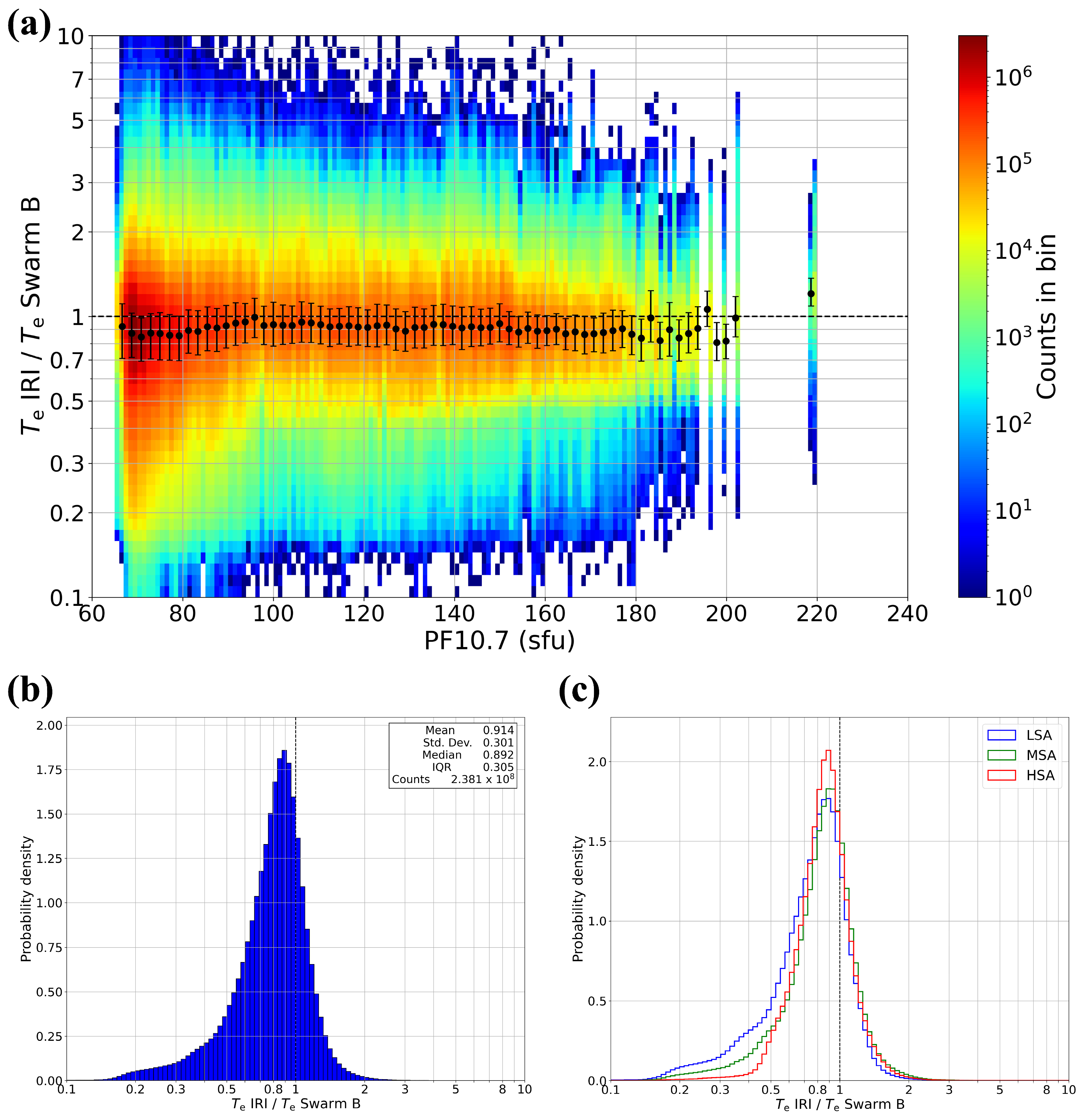
• The TBT-2012+SA model included in IRI-2020 shows different performances for mid- and high latitudes. While it correctly describes the T_e diurnal and seasonal variations for different solar activity levels at mid-latitudes, the steep and narrow high-latitude T_e enhancements found in the polar cusp region at noon and that associated with the sub-auroral enhancements at nighttime are not properly described. The model generally underestimates the observed T_e from Swarm B by about 10% on average, particularly for LSA and at high latitudes.

Although some clear patterns have been highlighted, the corresponding physical explanation requires additional studies complemented by other kinds of observations to properly characterize the diverse drivers affecting T_e variations. Since T_e and N_e are strongly coupled in the topside ionosphere, showing either a positive or a negative correlation depending on boundary conditions [59], a future investigation of N_e variations with solar activity would also improve the comprehension of the T_e variations found in the present study.

This study did not at all consider T_e variations with geomagnetic activity. Since this is an important source of T_e variations at high latitudes, both in terms of spatial patterns and magnitude, a comprehensive specification of topside ionosphere T_e variations as a function of geomagnetic activity is a future objective.

The comparison with results obtained via Swarm B observations highlighted how the TBT-2012+SA model, the default option of IRI-2020 to model the electron temperature, would benefit from the inclusion of Swarm satellite observations in its dataset to improve both the representation of T_e features at high latitudes and the description of the corresponding variation with solar activity.

References

1. Titheridge, J.E. Ion transition heights from topside electron density profiles. Planet. Space Sci. 1976, 24, 229–246. [Google Scholar] [CrossRef]
2. Kotov, D.V.; Truhlík, V.; Richards, P.G.; Stankov, S.; Bogomaz, O.V.; Chernogor, L.F.; Domnin, I.F. Night-time light ion transition height behaviour over the Kharkiv (50°N, 36°E) IS radar during the equinoxes of 2006–2010. J. Atmos. Sol.-Terr. Phys. 2015, 132, 1–12. [Google Scholar] [CrossRef]
3. Vaishnav, R.; Jin, Y.; Golam Mostafa, M.; Aziz, S.R.; Zhang, S.-R.; Jacobi, C. Study of the upper transition height using ISR observations and IRI predictions over Arecibo. Adv. Space Res. 2021, 68, 2177–2185. [Google Scholar] [CrossRef]
4. Truhlík, V.; Třísková, L.; Šmilauer, J. New advances in empirical modelling of ion composition in the outer ionosphere. Adv. Space Res. 2004, 33, 844–849. [Google Scholar] [CrossRef]
5. Bauer, S.J. Diffusive equilibrium in the topside ionosphere. Proc. IEEE 1969, 57, 1114–1118. [Google Scholar] [CrossRef]
6. Pignalberi, A.; Pezzopane, M.; Nava, B.; Coïsson, P. On the link between the topside ionospheric effective scale height and the plasma ambipolar diffusion, theory and preliminary results. Sci. Rep. 2020, 10, 17541. [Google Scholar] [CrossRef]
7. Rishbeth, H.; Garriott, O. Introduction to Ionospheric Physics. International Geophysics Series v. 14; Academic Press: New York, NY, USA, 1969. [Google Scholar]
8. Ratcliffe, J.A. An Introduction to the Ionosphere and Magnetosphere; Cambridge University Press: Cambridge, UK, 1972. [Google Scholar]
9. Willmore, A.P. Electron and ion temperatures in the ionosphere. Space Sci. Rev. 1970, 11, 607–670. [Google Scholar] [CrossRef]
10. Banks, P.M. The thermal structure of the ionosphere. Proc. IEEE 1969, 57, 258–281. [Google Scholar] [CrossRef]
11. Schunk, R.W.; Nagy, A.F. Electron temperatures in the region of the ionosphere: Theory and observations. Rev. Geophys. 1978, 16, 355–399. [Google Scholar] [CrossRef]
12. Bilitza, D. Electron and ion temperature data for ionospheric modelling. Adv. Space Res. 1991, 11, 139–148. [Google Scholar] [CrossRef]
13. Spenner, K.; Plugge, R. Empirical model of global electron temperature distribution between 300 and 700 Km based on data from Aeros-A. J. Geophys. 1979, 46, 43–56. [Google Scholar]
14. Brace, L.H.; Theis, R. Global empirical models of ionospheric electron temperature in the upper F-region and plasmasphere based on in situ measurements from the atmosphere explorer-c, isis-1 and isis-2 satellites. J. Atmos. Terr. Phys. 1981, 43, 1317–1343. [Google Scholar] [CrossRef]
15. Truhlik, V.; Bilitza, D.; Triskova, L. A new global empirical model of the electron temperature with the inclusion of the solar activity variations for IRI. Earth Planets Space 2012, 64, 531–543. [Google Scholar] [CrossRef]
16. Bilitza, D.; Pezzopane, M.; Truhlik, V.; Altadill, D.; Reinisch, B.W.; Pignalberi, A. The International Reference Ionosphere model: A review and description of an ionospheric benchmark. Rev. Geophys. 2022, 60, e2022RG000792. [Google Scholar] [CrossRef]
17. Truhlík, V.; Třísková, L.; Šmilauer, J.; Afonin, V. Global empirical model of electron temperature in the outer ionosphere for period of high solar activity based on data of three Intercosmos satellites. Adv. Space Res. 2000, 25, 163–169. [Google Scholar] [CrossRef]
18. Truhlík, V.; Třísková, L.; Šmilauer, J. Improved electron temperature model and comparison with satellite data. Adv. Space Res. 2001, 27, 101–109. [Google Scholar] [CrossRef]
19. Pignalberi, A.; Giannattasio, F.; Truhlik, V.; Coco, I.; Pezzopane, M.; Consolini, G.; De Michelis, P.; Tozzi, R. On the Electron Temperature in the Topside Ionosphere as Seen by Swarm Satellites, Incoherent Scatter Radars, and the International Reference Ionosphere Model. Remote Sens. 2021, 13, 4077. [Google Scholar] [CrossRef]
20. Brace, L.H.; Mayr, H.G.; Reddy, B.M. The early effects of increasing solar activity upon the temperature and density of the 1000-kilometer ionosphere. J. Geophys. Res. 1968, 73, 1607–1615. [Google Scholar] [CrossRef]
21. Evans, J.V. Seasonal and sunspot cycle variations of F Region electron temperatures and protonospheric heat fluxes. J. Geophys. Res. 1973, 78, 2344–2349. [Google Scholar] [CrossRef]
22. Mahajan, K.; Pandey, V. Solar activity changes in the electron temperature at 1000-km altitude from the Langmuir probe measurements on Isis 1 and Explorer 22 satellites. J. Geophys. Res. 1979, 84, 5885–5889. [Google Scholar] [CrossRef]
23. Brace, L.H.; Theis, R.; Hoegy, W.R. A global view of F-region electron density and temperature at solar maximum. Geophys. Res. Lett. 1982, 9, 989–992. [Google Scholar] [CrossRef]
24. Brace, L.H.; Theis, R.; Hoegy, W.R. Ionospheric electron temperature at solar maximum. Adv. Space Res. 1987, 7, 99–106. [Google Scholar] [CrossRef]
25. Bilitza, D.; Hoegy, W.R. Solar activity variations of ionospheric plasma temperatures. Adv. Space Res. 1990, 10, 81–90. [Google Scholar] [CrossRef]
26. Brace, L.H.; Theis, R.F. Global models of Ne and Te at solar maximum based on DE-2 measurements. Adv. Space Res. 1990, 10, 39–45. [Google Scholar] [CrossRef]
27. Otsuka, Y.; Kawamura, S.; Balan, N.; Fukao, S.; Bailey, G.J. Plasma temperature variations in the ionosphere over the middle and upper atmosphere radar. J. Geophys. Res. 1998, 103, 20705–20713. [Google Scholar] [CrossRef]
28. Sethi, N.K.; Pandey, V.K.; Mahajan, K.K. Seasonal and solar activity changes of electron temperature in the F-region and topside ionosphere. Adv. Space Res. 2004, 33, 970–974. [Google Scholar] [CrossRef]
29. Zhang, S.-R.; Holt, J.M. Ionospheric plasma temperatures during 1976–2001 over Millstone Hill. Adv. Space Res. 2004, 33, 963–969. [Google Scholar] [CrossRef]
30. Lei, J.; Roble, R.G.; Wang, W.; Emery, B.A.; Zhang, S.-R. Electron temperature climatology at Millstone Hill and Arecibo. J. Geophys. Res. 2007, 112, A02302. [Google Scholar] [CrossRef]
31. Bilitza, D.; Truhlik, V.; Richards, P.; Abe, T.; Triskova, L. Solar cycle variations of mid-latitude electron density and temperature: Satellite measurements and model calculations. Adv. Space Res. 2007, 39, 779–789. [Google Scholar] [CrossRef]
32. Truhlik, V.; Bilitza, D.; Třísková, L. Latitudinal variation of the topside electron temperature at different levels of solar activity. Adv. Space Res. 2009, 44, 693–700. [Google Scholar] [CrossRef]
33. Stolle, C.; Liu, H.; Truhlík, V.; Luehr, H.; Richards, P.G. Solar flux variation of the electron temperature morning overshoot in the equatorial F region. J. Geophys. Res. Space Phys. 2011, 116, A04308. [Google Scholar] [CrossRef]
34. Friis-Christensen, E.; Lühr, H.; Hulot, G. Swarm: A constellation to study the Earth’s magnetic field. Earth Planets Space 2006, 58, 351–358. [Google Scholar] [CrossRef]
35. Laundal, K.M.; Richmond, A.D. Magnetic coordinate systems. Space Sci. Rev. 2017, 206, 27–59. [Google Scholar] [CrossRef]
36. Knudsen, D.J.; Burchill, J.K.; Buchert, S.C.; Eriksson, A.I.; Gill, R.; Wahlund, J.; Åhlen, L.; Smith, M.; Moffat, B. Thermal ion imagers and Langmuir probes in the Swarm electric field instruments. J. Geophys. Res. Space Phys. 2017, 122, 2655–2673. [Google Scholar] [CrossRef]
37. Catapano, F.; Buchert, S.; Qamili, E.; Nilsson, T.; Bouffard, J.; Siemes, C.; Coco, I.; D’Amicis, R.; Tøffner-Clausen, L.; Trenchi, L.; et al. Swarm Langmuir probes’ data quality validation and future improvements. Geosci. Instrum. Methods Data Syst. 2022, 11, 149–162. [Google Scholar] [CrossRef]
38. Lomidze, L.; Knudsen, D.J.; Burchill, J.; Kouznetsov, A.; Buchert, S.C. Calibration and validation of swarm plasma densities and electron temperatures using ground-based radars and satellite radio occultation measurements. Radio Sci. 2018, 53, 15–36. [Google Scholar] [CrossRef]
39. Swarm L1b Product Definition. 2018. Available online: https://earth.esa.int/eogateway/documents/20142/37627/swarm-level-1b-product-definition-specification.pdf (accessed on 15 April 2024).
40. Pignalberi, A.; Coco, I.; Giannattasio, F.; Pezzopane, M.; De Michelis, P.; Consolini, G.; Tozzi, R. A new ionospheric index to investigate electron temperature small-scale variations in the topside ionosphere. Universe 2021, 7, 290. [Google Scholar] [CrossRef]
41. Pignalberi, A.; Habarulema, J.B.; Pezzopane, M.; Rizzi, R. On the development of a method for updating an empirical climatological ionospheric model by means of assimilated vTEC measurements from a GNSS receiver network. Space Weather 2019, 17, 1131–1164. [Google Scholar] [CrossRef]
42. Karpachev, A.T. Variations in the winter troughs’ position with local time, longitude, and solar activity in the Northern and Southern Hemispheres. J. Geophys. Res. Space Phys. 2019, 124, 8039–8055. [Google Scholar] [CrossRef]
43. Prölss, G.W. Subauroral electron temperature enhancement in the nighttime ionosphere. Ann. Geophys. 2006, 24, 1871–1885. [Google Scholar] [CrossRef]
44. Prölss, G.W. Electron temperature enhancement beneath the magnetospheric cusp. J. Geophys. Res. 2006, 111, A07304. [Google Scholar] [CrossRef]
45. Giannattasio, F.; De Michelis, P.; Pignalberi, A.; Coco, I.; Consolini, G.; Pezzopane, M.; Tozzi, R. Parallel electrical conductivity in the topside ionosphere derived from Swarm measurements. J. Geophys. Res. Space Phys. 2021, 126, e2020JA028452. [Google Scholar] [CrossRef]
46. Brinton, H.C.; Grebowsky, J.M.; Brace, L.H. The high-latitude winter F region at 300 km: Thermal plasma observations from AE-C. J. Geophys. Res. 1978, 83, 4767–4776. [Google Scholar] [CrossRef]
47. ISO 16457; Space Systems—Space Environment (Natural and Artificial)—The Earth’s Ionosphere Model: International Reference Ionosphere (IRI) Model and Extension to the Plasmasphere. International Standardization Organization: Geneva, Switzerland, 2022. Available online: http://www.iso.org/iso/home/store/catalogue_tc/catalogue_detail.htm?csnumber=61556 (accessed on 15 April 2024).
48. Bilitza, D. Models for Ionospheric Electron and Ion Temperature. In International Reference Ionosphere-IRI 79; Report, UAG-82; Rawer, K., Lincoln, J.V., Conkright, R.O., Eds.; World Data Center A for Solar-Terrestrial Physics: Boulder, CO, USA, 1981; p. 245. Available online: http://www.irimodel.org/ (accessed on 15 April 2024).
49. Bilitza, D.; Brace, L.; Theis, R. Modelling of ionospheric temperature profiles. Adv. Space Res. 1985, 5, 53–58. [Google Scholar] [CrossRef]
50. Richards, P.G.; Fennelly, J.A.; Torr, D.G. EUVAC: A solar EUV flux model for aeronomic calculations. J. Geophys. Res. 1994, 99, 8981–8992. [Google Scholar] [CrossRef]
51. Tapping, K.F. The 10.7 cm solar radio flux (F10.7). Space Weather 2013, 11, 394–406. [Google Scholar] [CrossRef]
52. Richards, P.G.; Woods, T.N.; Peterson, W.K. HEUVAC: A new high resolution solar EUV proxy model. Adv. Space Res. 2006, 37, 315–322. [Google Scholar] [CrossRef]
53. Booker, H.G. Fitting of multi-region ionospheric profiles of electron density by a single analytic function of height. J. Atmos. Terr. Phys. 1977, 39, 619–623. [Google Scholar] [CrossRef]
54. Pignalberi, A.; Aksonova, K.D.; Zhang, S.-R.; Truhlik, V.; Gurram, P.; Pavlou, C. Climatological study of the ion temperature in the ionosphere as recorded by Millstone Hill incoherent scatter radar and comparison with the IRI model. Adv. Space Res. 2021, 68, 2186–2203. [Google Scholar] [CrossRef]
55. Truhlik, V.; Bilitza, D.; Kotov, D.; Shulha, M.; Třísková, L. A global empirical model of the ion temperature in the ionosphere for the international reference ionosphere. Atmosphere 2021, 12, 1081. [Google Scholar] [CrossRef]
56. Evans, J. Theory and practice of ionosphere study by Thomson scatter radar. Proc. IEEE 1969, 57, 496–530. [Google Scholar] [CrossRef]
57. Schunk, R.; Nagy, A.F. Ionospheres: Physics, Plasma Physics, and Chemistry, 2nd ed.; Cambridge University Press: Cambridge, UK, 2009. [Google Scholar]
58. Třísková, L.; Truhlík, V.; Šmilauer, J. An empirical topside electron density model for calculation of absolute ion densities in IRI. Adv. Space Res. 2006, 37, 928–934. [Google Scholar] [CrossRef]
59. Pignalberi, A.; Giannattasio, F.; Truhlik, V.; Coco, I.; Pezzopane, M.; Alberti, T. Investigating the main features of the correlation between electron density and temperature in the topside ionosphere through Swarm satellites data. J. Geophys. Res. Space Phys. 2024, 129, e2023JA032201. [Google Scholar] [CrossRef]
60. Truhlik, V.; Třísková, L.; Bilitza, D.; Podolska, K. Variations of daytime and nighttime electron temperature and heat flux in the upper ionosphere, topside ionosphere and lower plasmasphere for low and high solar activity. J. Atmos. Sol.-Terr. Phys. 2009, 71, 2055–2063. [Google Scholar] [CrossRef]
61. Marif, H.; Lilensten, J. Suprathermal electron moments in the ionosphere. J. Space Weather Space Clim. 2020, 10, 22. [Google Scholar] [CrossRef]
62. Iijima, T.; Potemra, T.A. Large-scale characteristics of field-aligned currents associated with substorms. J. Geophys. Res. Space Phys. 1978, 83, 599–615. [Google Scholar] [CrossRef]
63. Heelis, R.A.; Hanson, W.B.; Burch, J.L. Ion convection velocity reversals in the dayside cleft. J. Geophys. Res. 1976, 81, 3803–3809. [Google Scholar] [CrossRef]
64. Titheridge, J.E. Ionospheric heating beneath the magnetospheric cleft. J. Geophys. Res. 1976, 81, 3221–3226. [Google Scholar] [CrossRef]
65. Liou, K.; Newell, P.T.; Meng, C.-I. Seasonal effects on auroral particle acceleration and precipitation. J. Geophys. Res. 2001, 106, 5531–5542. [Google Scholar] [CrossRef]
66. Liou, K.; Zhang, Y.-L.; Newell, P.T.; Paxton, L.J.; Carbary, J.F. TIMED/GUVI observation of solar illumination effect on auroral energy deposition. J. Geophys. Res. 2011, 116, A09305. [Google Scholar] [CrossRef]
67. Giannattasio, F.; Consolini, G.; Coco, I.; De Michelis, P.; Pezzopane, M.; Pignalberi, A.; Tozzi, R. Dissipation of field-aligned currents in the topside ionosphere. Sci. Rep. 2022, 12, 17202. [Google Scholar] [CrossRef] [PubMed]
68. Christiansen, F.; Papitashvili, V.O.; Neubert, T. Seasonal variations of high-latitude field-aligned currents inferred from Oersted and Magsat observations. J. Geophys. Res. 2002, 107, SMP 5-1–SMP 5-13. [Google Scholar] [CrossRef]
69. Wang, H.; Lühr, H.; Ma, S.Y. Solar zenith angle and merging electric field control of field-aligned currents: A statistical study of the Southern Hemisphere. J. Geophys. Res. 2005, 110, 306. [Google Scholar] [CrossRef]
70. Werner, S.; Prölss, G.W. The position of the ionospheric trough as a function of local time and magnetic activity. Adv. Space Res. 1997, 20, 1717–1722. [Google Scholar] [CrossRef]
71. Brace, L.H. Solar cycle variations in F-region Te in the vicinity of the midlatitude trough based on AE-C measurements at solar minimum and DE-2 measurements at solar maximum. Adv. Space Res. 1990, 10, 83–88. [Google Scholar] [CrossRef]
72. Fok, M.-C.; Kozyra, J.U.; Brace, L.H. Solar cycle variation in the subauroral electron temperature enhancement: Comparison of AE-C and DE 2 satellite observations. J. Geophys. Res. 1991, 96, 1861–1866. [Google Scholar] [CrossRef]
73. Fok, M.-C.; Kozyra, J.U.; Warren, M.F.; Brace, L.H. Seasonal variations in the subauroral electron temperature enhancement. J. Geophys. Res. 1991, 96, 9773–9780. [Google Scholar] [CrossRef]
74. Giannattasio, F.; Pignalberi, A.; De Michelis, P.; Coco, I.; Consolini, G.; Pezzopane, M.; Tozzi, R. Dependence of parallel electrical conductivity in the topside ionosphere on solar and geomagnetic activity. J. Geophys. Res. Space Phys. 2021, 126, e2021JA029138. [Google Scholar] [CrossRef]
75. Denton, M.H.; Bailey, G.J.; Su, Y.Z.; Oyama, K.-I.; Abe, T. High altitude observations of electron temperature and a possible north–south asymmetry. J. Atmos. Sol.-Terr. Phys. 1999, 61, 775–788. [Google Scholar] [CrossRef]
76. Laurenza, M.; Del Moro, D.; Alberti, T.; Battiston, R.; Benella, S.; Benvenuto, F.; Berrilli, F.; Bertello, I.; Bertucci, B.; Biasiotti, L.; et al. The CAESAR Project for the ASI Space Weather Infrastructure. Remote Sens. 2023, 15, 346. [Google Scholar] [CrossRef]
Figure 1. (Panel (a)) Time series of the daily solar activity index F10.7 (blue line), and the derived PF10.7 (red line) and F10.781 (green line) indices. Horizontal gray dashed lines set the solar activity thresholds used in this study. (Panel (b)) Time series of the Swarm B orbit height above Earth’s surface and local time at the geographic equator crossing point. The blue and red points are the heights, respectively, for ascending and descending orbits. Green and orange points are the local times, respectively, for ascending and descending orbits.
Atmosphere 15 00490 g001
Figure 2. Polar maps in MLT (hours) vs. QD latitude (degrees) of the mean electron temperature from the Swarm B LP observations recorded in the period of 2014−2023, as a function of the season. Polar maps encompass the QD latitudes from |30°| to the poles. The first-row plots are for the June solstice season (May, June, July, and August), the second row is for the December solstice season (November, December, January, and February), and the third row is for the combined equinoxes season (March, April, September, and October). The first-column plots are for the Northern Hemisphere, while the second column is for the Southern Hemisphere.
Atmosphere 15 00490 g002
Figure 3. Polar maps in MLT (hours) vs. QD latitude (degrees) of the mean electron temperature modeled by IRI along the Swarm B orbits recorded in the period of 2014−2023, as a function of the season. Polar maps encompass the QD latitudes from |30°| to the poles. The first-row plots are for the June solstice season (May, June, July, and August), the second row is for the December solstice season (November, December, January, and February), and the third row is for the combined equinoxes season (March, April, September, and October). The first-column plots are for the Northern Hemisphere, and the second column is for the Southern Hemisphere.
Atmosphere 15 00490 g003
Figure 4. (First-column plots) Polar maps in MLT vs. QD latitudes of the mean electron temperature from the Swarm B LP observations recorded in the period of 2014−2023, for the December solstice season (November, December, January, and February) and the Southern Hemisphere, as a function of solar activity level. Polar maps encompass the QD latitudes from 30° S to the south geomagnetic pole. The top plot is for low solar activity, the middle plot is for medium solar activity, and the bottom plot is for high solar activity. (Second-column plots) Polar maps of percentage residuals between electron temperature means recorded at a different solar activity level. Specifically, the top plot is for the percentage residuals between the low and medium solar activity levels, the middle plot is for the percentage residuals between the high and medium solar activity levels, and the bottom plot is for the percentage residuals between the high and low solar activity levels. (Third-column plots) Mean zonal, i.e., latitudinal, (solid lines) and standard deviation (shaded area) electron temperature values for three different latitudinal ranges and for different solar activity levels (blue for low, green for medium, and red for high solar activity). From top to bottom: polar cusp, mid-latitude ionospheric trough, and mid-latitudes.
Atmosphere 15 00490 g004
Figure 5. Same as Figure 4 but for the June solstice season (May, June, July, and August).
Atmosphere 15 00490 g005
Figure 6. Same as Figure 4 but for the equinox seasons (March, April, September, and October).
Atmosphere 15 00490 g006
Figure 7. (First-column plots) Polar maps in MLT vs. QD latitudes of the mean electron temperature modeled by IRI along the Swarm B orbits recorded in the period of 2014−2023, for the December solstice season (November, December, January, and February) and the Southern hemisphere, as a function of solar activity level. Polar maps encompass the QD latitudes from 30° S to the south geomagnetic pole. The top plot is for low solar activity, the middle plot is for medium solar activity, and the bottom plot is for high solar activity. (Second-column plots) Polar maps of percentage residuals between electron temperature means recorded at a different solar activity level. Specifically, the top plot is for the percentage residuals between the low and medium solar activity levels, the middle plot is for the percentage residuals between the high and medium solar activity levels, and the bottom plot is for the percentage residuals between the high and low solar activity levels. (Third-column plots) Mean zonal, i.e., latitudinal, (solid lines) and standard deviation (shaded area) electron temperature values for four different latitudinal ranges and for different solar activity levels (blue for low, green for medium, and red for high solar activity). From top to bottom: polar cusp, mid-latitude ionospheric trough, and mid-latitudes.
Atmosphere 15 00490 g007
Figure 8. Same as Figure 7 but for the June solstice season (May, June, July, and August).
Atmosphere 15 00490 g008
Figure 9. Same as Figure 7 but for the equinox seasons (March, April, September, and October).
Atmosphere 15 00490 g009
Figure 10. Panel (a) shows the ratios between the IRI-modeled and Swarm B-measured electron temperature values as a function of the PF10.7 solar activity proxy. The data from the entire dataset (2014–2023) in the range of QD latitudes from |30°| to the geomagnetic poles have been used. Colors represent the counts inside each bin on a logarithmic scale. Black points and error bars represent the median and inter-quartile range values for different PF10.7 ranges. The horizontal black dashed line represents the value of the ratio equal to one. Panel (b) shows the probability density histogram of the ratio values represented in panel (a). The vertical black dashed line represents the value of the ratio equal to one. The statistical parameters of the ratio distribution are reported in the upper right box. Panel (c) shows the probability density histograms of the ratio values as a function of solar activity: blue for LSA, green for MSA, and red for HSA.
Atmosphere 15 00490 g010
Figure 11. Comparison among electron temperature values recorded by the Millstone Hill ISR (boxplots), Swarm B LP (black lines), and modeled by IRI (green lines), as a function of the magnetic local time, for the altitude range of 510 ± 20 km. Panels (ac) represent the equinoxes, June solstice, and December solstice seasons, respectively, for low-solar-activity conditions. Panels (df) are for medium-solar-activity conditions, while panels (gi) are for high-solar-activity conditions. In the boxplot representation, the red line is the median value (50th percentile), the blue box is the inter-quartile range (25th to 75th percentiles), and the lower and upper blue whiskers are the 5th and 95th percentiles, respectively. The yellow bar plots represent the counts of ISR’s observations in the bin. The Swarm B and IRI lines are the median values calculated from the data recorded at the ISR QD latitude as a function of MLT, for the selected seasons and solar activity level.
Atmosphere 15 00490 g011
Disclaimer/Publisher’s Note: The statements, opinions and data contained in all publications are solely those of the individual author(s) and contributor(s) and not of MDPI and/or the editor(s). MDPI and/or the editor(s) disclaim responsibility for any injury to people or property resulting from any ideas, methods, instructions or products referred to in the content.