Abstract
The atmospheric flow field and weather processes exhibit complex and variable characteristics at small scales, involving interactions between terrain features and atmospheric physics. To investigate the mechanisms of these process further, this study employs a Lagrangian particle motion model combined with a Euler background field approach to construct a small-scale atmospheric flow field model. The model streamlines the modeling process by combining the benefits of the Lagrangian dynamics model and the Eulerian integration scheme. To verify the effectiveness of the Euler–Lagrange hybrid model, experiments using the Fluent wind field model were conducted for comparison. The results show that both models have their advantages in handling terrain-induced wind fields. The Fluent model excels in simulating the general characteristics of wind fields under specific terrain, while the Euler–Lagrange hybrid model is better at capturing the upstream and downstream disturbances of the terrain on the atmospheric flow field. These findings provide powerful tools for in-depth diagnostic analysis of atmospheric flow simulation and convective precipitation processes. Notably, the Euler–Lagrange hybrid model demonstrates excellent computational efficiency, with an average computation time of approximately 2 s per time step in a Python environment, enabling rapid simulation of 40 time steps within approximately 90 s.
1. Introduction
In recent years, research on mesoscale and small-scale weather processes has received increasing attention [1]. Due to the suddenness and rapid evolution of these processes [2], forecasting becomes significantly challenging [3]. Particularly during the rainy season or flood season, local atmospheric flow fields are profoundly influenced by complex terrain factors, making them prone to triggering small-scale severe convective weather processes in a very short time [4], leading to secondary disasters, such as heavy rain, debris flows, and floods, resulting in casualties and property losses [5]. Therefore, the study of mesoscale and small-scale weather processes holds notable scientific significance and practical value [6].
The study of small-scale weather processes faces multiple challenges [7], primarily manifested in the following aspects: a. the dynamic mechanisms are extremely complex, involving interactions of various physical processes that are difficult to accurately describe; b. the precipitation triggering and formation mechanisms remain unclear and lack in-depth theoretical and experimental support; c. There is a scarcity of observational data due to the suddenness and localized nature of small-scale weather processes, greatly increasing the difficulty of field observations and making it extremely challenging to obtain observational data [8]. Additionally, mainstream meteorological models such as WRF [9] perform well in simulating mesoscale weather processes but struggle to achieve dynamic accuracy for small-scale regions [10]. Therefore, it is necessary to further implement dynamic downscaling based on the WRF model to more accurately characterize and predict small-scale weather processes [11].
The mainstream dynamic atmospheric model framework, based on the Euler method [12] and employing a terrain-following coordinate system, solves the atmospheric motion equations by constructing staggered grids to simulate atmospheric flow fields [13]. From the Euler perspective, the modeling schemes of mesoscale meteorological models are quite mature. However, in small-scale numerical simulations, especially under complex terrain conditions, atmospheric motion is influenced by terrain disturbances, and the terrain-following coordinate system may not fully capture these complex influences, leading to inadequate accuracy of simulation results [14]. Therefore, for small-scale numerical simulations, further exploration of more suitable coordinate systems and numerical methods is needed to more accurately describe and predict meteorological phenomena under complex terrain conditions.
In order to accurately simulate the characteristics of atmospheric flow fields under complex terrain conditions, this study adopts a z-coordinate system to construct the atmospheric flow field. To simplify the numerical model, this paper abandons the purely Euler-based simulation approach and instead adopts an Euler–Lagrange combined method to build a small-scale atmospheric dynamics model. The core idea of this method is to treat air masses as particle points [15] and solve the atmospheric motion equations by simulating the movement of particle groups [16].
Specifically, in the Euler–Lagrange method, the motion state of particle groups is first computed, and then this motion information is fed back to the atmospheric background grid [17]. Based on the spatial force distribution characteristics of the background grid, the motion characteristics of particles are further derived [18]. This method achieves numerical simulation and prediction of atmospheric phenomena through the interaction between particles and the grid.
Traditional Euler methods require the use of staggered grids to compute the state of motion in space. In contrast, the Euler–Lagrange modeling approach utilizes the offset relationship between discrete particles and the background grid to replace the function of staggered grids, thereby reducing the complexity of numerical modeling and enhancing the efficiency of model construction to a certain extent.
Atmospheric dynamic models have extensive applications in meteorology. The Euler–Lagrange integration scheme serves as both a diagnostic model for wind fields and a downscaling model for atmospheric dynamics. It can be used to correct localized gridded wind fields, thereby providing more accurate background wind data for applications such as radar echo extrapolation and the dispersion of atmospheric pollutants, ultimately enhancing the accuracy of forecasts. Additionally, the Euler–Lagrange integration scheme can also serve as an alternative for small-scale meteorological models, providing theoretical support for urban weather forecasting and early warning systems for small basin flash floods [19]. Experiments conducted with the Euler–Lagrange integration scheme have demonstrated its practical value in meteorological modeling.
2. Model Design
The Euler–Lagrange hybrid algorithm model utilizes two systems, motion particles, and background grids, to describe atmospheric flow fields. As illustrated in Figure 1, particle points are placed within the background grid. The term “grid node” in Figure 1 denotes the grid nodes used to store grid point information.
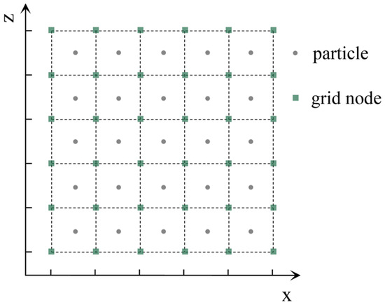
Figure 1.
Schematic diagram of the Euler–Lagrange hybrid model.
Particles are responsible for simulating atmospheric motion, while the grid is primarily used for calculating particle forces and solving spatial gradients. The model updates the background grid based on the virtual movement of particles, thereby providing feedback on motion information to the grid.
2.1. Modeling Equations
In small-scale meteorological models, air parcels are influenced by wind field disturbances during atmospheric motion, causing pressure fluctuations and thereby altering their motion states. Assuming expansion or compression of the air parcel in the x-direction within a unit time, the volume change in the air parcel is provided by [20]:
The volume change in the air parcel after expansion or compression in the x and z directions is then provided by the following equation:
According to the ideal gas equation p0·V0 = p1·V1, it is evident that pressure changes are related to volume changes. Thus, p1 = p0·V0/V1, yielding the following equation:
The pressure difference before and after the change in air parcel state within a unit time can be obtained as follows:
Here, δp refers to the atmospheric pressure disturbance quantity within a unit time.
Deformation gradient (C): a physical quantity describing the tendency of deformation of fluid elements. The calculation formula for the deformation gradient is as follows:
Deformation variable (J): a physical quantity describing the extent of deformation of fluid elements within a time step. The calculation formula is as follows:
When the strain measure J > 1, it indicates air parcel expansion; when J < 1, it indicates air parcel compression; and when J = 1, it indicates no change in air parcel volume.
Disturbance pressure (δp): atmospheric pressure fluctuations generated by the motion of air parcels, which can also be approximated as the following:
Atmospheric motion equation: in small-scale meteorological models, the movement of air parcels is mainly influenced by atmospheric pressure disturbances [21]. It is assumed that in the vertical direction, gravity is balanced by atmospheric static pressure.
where λ represents the grid adaptation parameter, Fx and Fz denote the frictional resistance of air parcels in the horizontal and vertical directions, ρ represents air density, (u, w) represent wind speeds, θmean represents the mean potential temperature, and θ′ represents the potential temperature perturbation.
Pressure equation: The variation of pressure over time in the background grid. The calculation formula is [22]:
where g represents gravity. This formula can be used to calculate the pressure changes during the Lagrangian particle displacement process.
Temperature equation: a physical quantity describing the variation of temperature with changes in motion state. The calculation formula is [23]:
where cp represents the specific heat capacity of air, cp = 1005 J/(kg·K), Lv denotes the latent heat of water vapor, and where the standard atmospheric pressure Lv = 2260 kJ/kg. This formula can be used to calculate the temperature changes during the Lagrangian particle displacement process.
2.2. Calculation of Spatial Gradient Forces
In the Euler perspective, deformation of computational grid points is commonly employed to calculate the pressure gradient forces between grids. However, in the Euler–Lagrange model perspective, it is necessary to first calculate the deformation of Lagrangian particles and then apply the pressure gradient forces from the Lagrangian particle deformation to the grid [24].
- (I)
- Deformation Calculation
In the Euler perspective, meteorological models employ the finite difference method to calculate deformation, expressed as follows:
In the Euler perspective, ∂/∂x can be resolved through differencing operations among adjacent grid points i, i + 1, i − 1.
In contrast, within the Euler–Lagrange model perspective, particles inherently possess attributes such as air pressure, temperature, and deformation. As these particles expand or undergo compression, the resulting pressure gradient forces they generate are then fed back to the background grid [25].
In Figure 2, particle A is positioned between grid points i and i + 1. When there is a velocity difference between point i and point i + 1, it can be inferred that particle A undergoes deformation. The formula for calculating the deformation gradient of particle A is as follows [26]:
where Ui represents the velocity of grid point i, Δx denotes the grid spacing, and Wi indicates the weighting factor of grid point i on particle A. The distance between particle A and grid point i is denoted as dA,i, with dA,i = xi − xA. In Figure 2, there are two grid points, i and i + 1, near particle A, thus dA,i < 0 and dA,i+1 > 0.
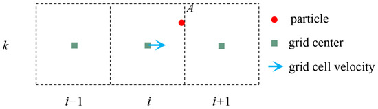
Figure 2.
Calculation of particle deformation using grid point velocities.
By utilizing Equation (13), the deformation of particle A can be calculated, thereby determining whether particle A is in a state of compression or expansion. Based on this deformation state and according to Equation (7), the perturbation pressure generated by the particle due to its compression or expansion can be computed, yielding the perturbation pressure δpA of particle A.
- (II)
- Calculation of Pressure Gradient Forces
In the Euler–Lagrange hybrid model, the pressure gradient forces acting on grid points are determined by the surrounding particle pressures [27]. In Figure 3, green squares represent the centers of grid points, while colored dots represent Lagrange particles.
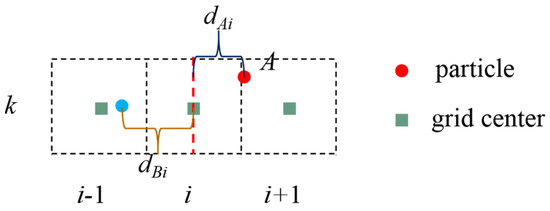
Figure 3.
Spatial relationship between particles and grid point centers.
Assuming there are two particle points, A and B, near grid point i, after calculating the deformation gradient C and perturbation pressure δp of the particle points, the perturbation pressure of the particle points will be applied to the background grid. If particle point A is to the right of grid point i, then the gradient force exerted by particle point A on grid point i is represented as [28]:
Here, d′A,i = xA − xi represents the distance relationship; and δpA denotes the perturbation pressure generated by the compression or expansion of particle A itself.
If particle point A is to the left of grid point i + 1, then the gradient force exerted by particle point A on grid point i + 1 is represented as follows:
If there are multiple particles around grid point i, then the gradient force acting on grid point i can be represented as follows:
Herein, n denotes the number of particles surrounding grid point i, p represents the p-th particle around grid point i, d′pi = xp − xi represents the distance (including sign) between the p-th particle and grid point i, and Wp denotes the weight coefficient between particle p and grid point i. It is necessary to ensure that the sum of the weights of the particles around grid point i equals 1, as expressed in Equation (17):
This calculation yields the spatial acceleration of the background field.
- (III)
- Calculation of Gradient Forces near Terrain
The Lagrange method is more flexible in handling terrain rebound.
As shown in Figure 4, the grid point (i − 1,k) represents an air grid point, while the grid point (i,k) represents a terrain grid point with a velocity of 0. The velocity corresponding to grid point (i,k) is denoted as ui,j. In Figure 4a, when ui−1,j > 0 and ui,j = 0, based on the velocity difference of neighboring grid points around particle A, it can be inferred that particle A is under compression. Similarly, in Figure 4b, when ui−1,j < 0 and ui,j = 0, based on the velocity difference of neighboring grid points around particle A, it can be inferred that particle A is under expansion. According to Equation (13), the deformation gradient of particle A can be computed for both states depicted in Figure 4a,b.
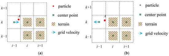
Figure 4.
Two states of particle A: (a) particle A is compressed; (b) particle A is expanded.
Based on the deformation gradient of particle A, the perturbed air pressure exerted by particle A itself can be computed, enabling the calculation of the pressure gradient forces applied by particle A on grid points (i − 1,k) and (i,k), thus updating the spatial force relationships of the background grid. Through this approach, the pressure interactions between particles and terrain have been effectively addressed.
- (IV)
- Model Computation Process
In the traditional Eulerian framework for dynamic models, staggered grids are typically employed to separately compute the pressure and vector fields. In contrast, the Euler–Lagrange hybrid model utilizes the misalignment relationship between particles and the background grid to replace staggered grids, thereby reducing the complexity of model construction.
Figure 5 illustrates the computational workflow within a single time step; this includes the following steps:
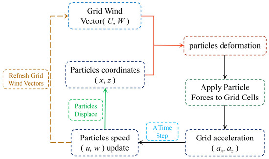
Figure 5.
Computational flowchart for a single time step.
- Calculation of particle deformation: particle coordinates are used to aggregate wind vectors from surrounding grid points, enabling the computation of particle deformation;
- Application of gradient forces from particle deformation to the background grid;
- Acquisition of acceleration by background grid points, with the acceleration projected onto particles;
- Update of particle velocities and calculation of particle displacement over a single time step;
- Update of background grid velocities.
These steps collectively complete the iterative process for a single time step.
2.3. Lagrange Method for Particle Motion Computation
From the Lagrangian perspective, particle motion is determined by its initial velocity and the gradient forces provided by the background grid.
- (I)
- Particle Motion
According to Newton’s equations of motion, the following equation holds true:
Here, u0 and u1 represent the velocity of the particle at the initial and final time steps within the time interval, while the acceleration (a) is provided by the gradient forces from the background grid.
- (II)
- Mapping Particle Momentum to Adjacent Grid Points
After one time step, the particle’s velocity and coordinates undergo changes.
Figure 6a illustrates the mapping of particle momentum to the background grid, thereby updating the momentum field of the background grid. Assuming there are (n) particles near the grid point, the momentum mapped to the grid point by these particles is [29]:
where Wsum represents the sum of weights, pg denotes the momentum mapped to the grid point, mi·vi represents the momentum of the i-th particle, and Wi represents the weight coefficient of the i-th particle relative to the grid point.
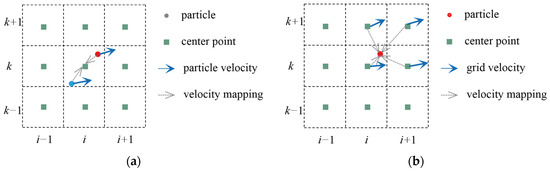
Figure 6.
(a) Mapping of particle velocities to grid points; (b) mapping of grid point velocities to particles.
- (III)
- Mapping Grid Point Momentum to Particles
The equation for mapping grid point momentum to particles is [30]:
Here, Wsum represents the sum of weights, the subscript (i, k) denotes the indices of grid points near the particle, and ellipses indicate the traversal of grid points near the particle. Wi,k represents the weight coefficient between the particle and its adjacent grid points. This formulation yields the momentum mapped from grid points to the particle, as shown in Figure 6b.
Mapping grid point mass near particles to particles is carried out using the following equation:
The mapped velocity is obtained:
2.4. Weight Calculation
The Euler–Lagrange model involves data mapping between particle clusters and grids. In this study, tricubic spline interpolation functions are employed to compute the data mapping relationship between particles and grid points [31].
In the equation, h is typically understood as 1.1 to 1.2 times the average grid spacing, and q represents the relative distance between particles and grid points. For the x-direction, the formula for calculating q is as follows:
Similarly, the formula for calculating (q) in the z-direction is analogous.
2.5. Boundary Conditions
In the Eulerian grid, boundary conditions are represented by boundary grids. In contrast, the Euler–Lagrange model employs moving particles to substitute for these boundary grids, which are referred to as “boundary particles”. The boundary particles are in a state of uniform motion. Upon entering the computational domain, the spatial acceleration of the boundary particles must be calculated, as shown in Figure 7. Due to the dynamic nature of the boundary particles, their position information needs to be reinitialized every n time steps.
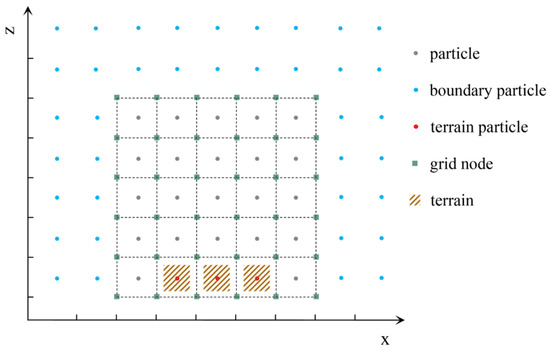
Figure 7.
Background grid and boundary conditions.
In the model, it is assumed that each terrain grid point corresponds to a virtual “particle”, referred to as a “terrain particle”. These “terrain particles” have a constant velocity of 0 but possess deformation values. This setup facilitates the computation of pressure gradient forces at the interface between the air and terrain.
Through this approach, the boundary conditions of the model are established.
2.6. Model Grid Scheme
In this study, a structured grid is employed to construct the atmospheric flow field. A Cartesian coordinate system is utilized in the 2D plane along the x and z directions, with uniform grid spacing set as dx in the x direction and dz in the z direction. The grid points are constructed using uniformly sized cubes. Each grid point is labeled according to its type, such as “air” or “terrain”. Particle-based displacement and deformation are utilized in this study to replace the functionality of staggered grids in traditional Eulerian frameworks.
2.7. Time Step Constraint
The selection of the time step must satisfy the Courant–Friedrichs–Lewy (CFL) condition, which stipulates that the product of the time step (δt) and the characteristic velocity (c) should not exceed the spatial step (δx). Therefore, the maximum time step is determined as follows:
Here, lmin represents the minimum grid spacing, and vmax denotes the maximum velocity. Typically, the minimum grid spacing in meteorological models is 400 m. In this experiment, the maximum wind vector does not exceed 10 m/s. Consequently, the threshold for the time step can be considered as 40 s.
2.8. Model Validation Scheme
Within this experiment, the Euler–Lagrange model utilized a 2D plane modeling in the x-z coordinate system, whereas mainstream meteorological models are typically three-dimensional. Therefore, there are certain limitations in the comparison of flow fields.
To facilitate experimental comparisons, the Fluent model [32] was chosen as an alternative approach in this study.
As a well-regarded atmospheric dynamic downscaling model, Fluent is widely employed in research pertaining to meteorological wind field downscaling [33]. It facilitates convenient simulation of 2D atmospheric flow fields and possesses the capability to adapt to resolutions ranging from meters to kilometers. Compared to mainstream meteorological models like WRF, Fluent demonstrates excellent performance under complex environmental conditions, offering researchers higher precision and reliability [34]. Consequently, scholars utilize Fluent as one of the dynamic downscaling tools for mesoscale models [35], enabling the calculation of wind fields under complex environmental conditions [36].
Considering these features of the Fluent model, this study employs its simulated wind field data for experimental comparison.
Due to the strengths of the Fluent model, this study uses its simulated wind field data for the comparative experiment.
2.9. Model Configuration
The experimental design employs a 2D plane atmospheric background field in the x-z coordinate system, establishing orthogonal grids and constructing an ideal experiment. It investigates the suitability of the Euler–Lagrange integration scheme for simulating atmospheric flow fields and the movement of atmospheric flow fields under complex terrain conditions.
Typically, the horizontal resolution of small-scale meteorological models ranges from 0.4 to 1 km. Therefore, this study sets the horizontal resolution of the Euler–Lagrange model at 800 m, vertical resolution at 400 m, and time step at 15 s. Using this configuration, this study simulates the flow characteristics of atmospheric wind fields under virtual terrain conditions.
The time step of the Fluent model is also set to 15 s, but Fluent allows for specifying the number of iterations within each time step.
3. Results
This study employs the Euler–Lagrange integration scheme to model and solve the atmospheric motion equations under small-scale conditions, exploring its applicability in atmospheric modeling. The Fluent model is utilized to simulate wind fields under identical terrain conditions.
3.1. Terrain Wind Characteristics
Using the terrain conditions illustrated in Figure 6, assuming u = 5 m/s and w = 0 m/s at t = 0 s, with a time step of dt = 15 s, the atmospheric flow field evolves over time.
To validate the accuracy of the Euler–Lagrange model within a single time step, we designed the following experimental setup:
Experiment a: we computed the results after one time step using the Euler–Lagrange model.
Experiment b: we computed the results after one time step using the Fluent model.
Experiment c: we computed the results after five iterations within one time step using the Fluent model (dividing the time step into five intervals).
Experiment d: we calculated the difference between the results of Experiment b and Experiment a.
Experiment e: we calculated the difference between the results of Experiment c and Experiment a.
The experimental sequence corresponds directly to the labeling of the subfigures in Figure 8.
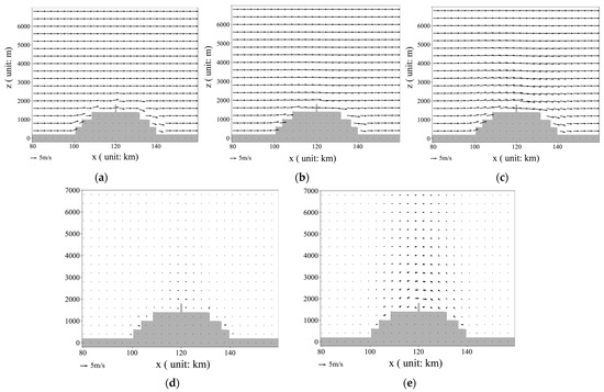
Figure 8.
Wind fields at t = 15 s. (a) Wind field output by the Euler–Lagrange model; (b) wind field with 1 iteration per time step in the Fluent model; (c) wind field with 5 iterations per time step in the Fluent model; (d) difference between the results shown in (a,b); (e) difference between the results shown in (a,c).
In Figure 8a, the results of the Euler–Lagrange model for a single time step exhibit characteristics of the terrain wind field that are comparable to experimental condition b, with the perturbation intensity weaker than in experimental condition c. This suggests the feasibility of the Euler–Lagrange model’s time-stepping scheme for simulating terrain wind fields.
At t = 450 s, as shown in Figure 9, both models exhibit similar trend characteristics, but there are discrepancies in the results. The Euler–Lagrange model shows a slight decrease in wind speed in the lower and upper reaches near the terrain obstruction, which aligns with real atmospheric conditions. In contrast, the Fluent model indicates an enhancement in wind speed near the terrain. This discrepancy may stem from the Fluent model’s principle, which simulates according to wind tunnel assumptions. In wind tunnels, airflow continuously enters at a constant velocity, leading to enhanced wind speeds near terrain obstacles due to the pushing effect of the inlet airflow.
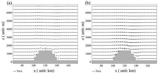
Figure 9.
Wind fields at t = 450 s. (a) Wind field output by the Euler–Lagrange model; (b) wind field output by the Fluent model.
At t = 900 s, as shown in Figure 10, the Euler–Lagrange model indicates that the terrain-induced wind field gradually propagates in the lee of the mountain. However, there is little change in the Fluent model results between t = 450 s and t = 900 s, and the downstream transmission of terrain disturbances in the Fluent model is not significant.
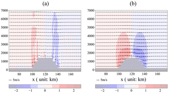
Figure 10.
Wind fields at t = 900 s, with filled contour lines indicating the distribution of vertical wind speed. (a) Wind field output by the Euler–Lagrange model; (b) wind field output by the Fluent model.
At t = 1350 s and t = 1800 s, as shown in Figure 11, the Euler–Lagrange model indicates oscillating airflow above the terrain, propagating downstream along the wind direction. Due to the lack of significant changes in wind field characteristics observed in the Fluent model at preceding and subsequent moments, related results are not further presented.
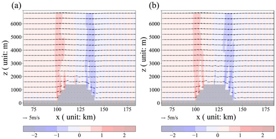
Figure 11.
Wind fields output by the Euler–Lagrange model, with filled contour lines indicating the distribution of vertical wind speed. (a) Wind field at t = 1350 s; (b) wind field at t = 1800 s.
At t = 2025 s and t = 2475 s, as shown in Figure 12, the Euler–Lagrange model indicates continuous airflow disturbances near the terrain, with these disturbed airflows propagating downstream along the wind direction.
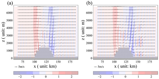
Figure 12.
Wind fields output by the Euler–Lagrange model, with filled contour lines indicating the distribution of vertical wind speed. (a) Wind field at t = 2025 s; (b) wind field at t = 2475 s.
In general, terrain-induced wind fields generate oscillating airflows downstream, commonly known as “terrain waves” [37], which gradually propagate downstream and cause disturbances [38]. Terrain waves are a common phenomenon in mountainous airflow, making complex terrain prone to triggering convective weather processes and even precipitation [39]. During the propagation of terrain wave airflow, kinetic energy in the wind field dissipates. The Euler–Lagrange model used in this study effectively simulates terrain wave disturbances, consistent with the characteristics of atmospheric flow fields [40].
3.2. Simulation of Canyon Terrain Wind Fields
To further validate the adaptability of the Euler–Lagrange model to complex terrain, the experiment constructed a canyon-like terrain.
Using the terrain conditions depicted in Figure 13, assuming uniform settings of u = 5 m/s and w = 0 m/s at t = 0 s, with a time step of dt = 15 s, flow field changes were observed after 15 s.
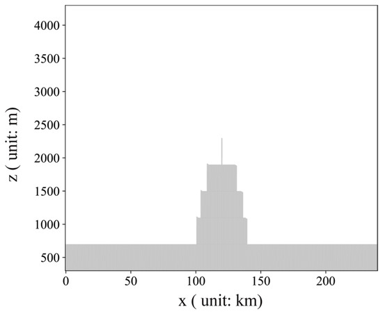
Figure 13.
Simulation of canyon terrain.
At t = 15 s, as shown in Figure 14, both models gradually adapt to the wind field under canyon terrain conditions.
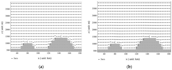
Figure 14.
Canyon terrain wind field at t = 15 s. (a) Wind field output from the Euler–Lagrange model; (b) wind field output from the Fluent model.
At t = 900 s, as shown in Figure 15, the fluctuation range of the terrain-disturbed wind field expands gradually.
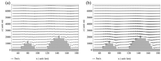
Figure 15.
Canyon terrain wind field at t = 900 s. (a) Wind field output from the Euler–Lagrange model; (b) wind field output from the Fluent model.
At t = 1800 s, as shown in Figure 16, the results from the Euler–Lagrange model indicate that the terrain wind field disturbance gradually propagates downstream, forming waves downstream. In comparison, the Fluent model’s wind field disturbance mainly concentrates near the mountain and shows no significant change over time.
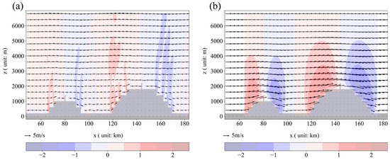
Figure 16.
Canyon terrain wind field at t = 1800 s. (a) Wind field output from the Euler–Lagrange model; (b) wind field output from the Fluent model.
At t = 2250 s, as shown in Figure 17, the Euler–Lagrange model results reveal significant “terrain waves” downstream, particularly in the canyon area between the two mountains, with more pronounced disturbance effects propagating downstream. In contrast, the Fluent model results indicate that after adapting to the terrain, the wind field does not exhibit distinct temporal variations.
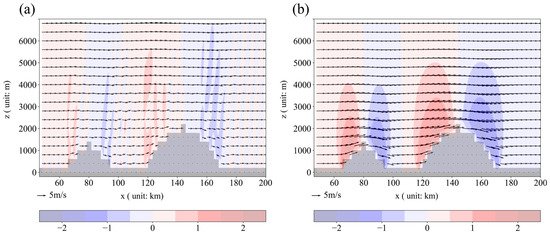
Figure 17.
Canyon terrain wind field at t = 2250. (a) Wind field output from the Euler–Lagrange model; (b) wind field output from the Fluent model.
Comparing the two simulation approaches for atmospheric flow under canyon terrain conditions, the Fluent model demonstrates rapid computation of complex terrain feedback on the wind field. However, since Fluent is not inherently a meteorological model, specific atmospheric flow characteristics at weather scales are automatically filtered during the simulation of atmospheric flow.
The Euler–Lagrange model can rapidly provide feedback when dealing with complex terrain and simulate the process of terrain wave disturbance propagating downwind, consistent with general atmospheric dynamics. Studies indicate that [41] during the rainy season or flood period, canyon terrain areas are prone to triggering precipitation processes, closely linked to terrain wave disturbances.
3.3. Model Computational Efficiency
To assess the model’s computation speed, this study recorded the model’s computation time. The equipment model used was the Xeon E5 2650, and the model programming language used was Python combined with the CuPy computing library. This paper compiled statistics on the number of iteration time steps and the corresponding consumed time.
From Table 1, it can be observed that the model consumes an average of approximately 2 s per time step. Considering the model’s implementation in Python, there is still room for improvement in computational efficiency.

Table 1.
Iteration count and time consumption.
3.4. Research Limitations
The experiments in this paper also have certain limitations, including the following points:
- Due to the difficulty in obtaining real-time data for small-scale meteorological wind fields and the fact that mainstream meteorological models are 3D models, while the model developed in this experiment is a 2D model, this paper compared the results by assuming virtual terrain conditions and using Fluent to simulate 2D flow fields.
- In practical downscaling processes, typically, a mesoscale model outputs a time series file every 3 to 5 min. Then, a downscaling model calculates the changes in atmospheric wind fields, temperature, and other physical processes within the 3 to 5 min interval. This process continues by reading new mesoscale data files for the next downscaling cycle. However, in this study, to test the model’s computational effectiveness and stability, an initial field was set, and the atmospheric state changes were estimated iteratively. The longest duration was 2500 s. Prolonged durations accumulate too much error, which affects the results.
- The main purpose of the experiments in this paper is to test the applicability of the Euler–Lagrange model under complex terrain conditions. The effectiveness of the theory and methods used in this paper awaits further validation through more extensive, representative, and rigorous experiments.
4. Discussion
The Euler–Lagrange integration scheme describes atmospheric motion using particle dynamics, endowing these particles with properties such as velocity and deformation, thereby replacing the staggered grids in traditional Eulerian models and simplifying the complexity of model construction. This approach demonstrates a high degree of adaptability in handling meteorological wind fields over complex terrain, making it suitable for applications in wind field diagnostic models or atmospheric dynamic downscaling models, thereby providing technical support for related domains.
In short-term forecasting, radar echo extrapolation relies on gridded wind field information. However, the construction of gridded wind field vectors involves interpolation of station data, inevitably introducing errors. Therefore, the Euler–Lagrange integration scheme can serve as a wind field diagnostic model to dynamically correct gridded data, thus improving the accuracy of short-term forecasts.
Similarly, in the field of atmospheric pollutant dispersion, wind field diagnostic models are crucial for improving and enhancing simulation accuracy. The Euler–Lagrange integration scheme also demonstrates its potential in this area.
In fields such as urban meteorological forecasting and small watershed flash flood warnings, there is a need for small-scale dynamic models to accurately capture meteorological changes under complex terrain conditions, thereby improving the efficiency of precipitation forecasts and enhancing meteorological service capabilities. The Euler–Lagrange integration scheme can serve as one of the alternative options for these small-scale dynamic models, contributing to the efficiency of precipitation forecasts and enhancing meteorological service capabilities.
5. Conclusions
This paper proposes the use of the Euler–Lagrange integration scheme to model atmospheric dynamics in small-scale scenarios, aiming to explore its applicability under complex terrain conditions.
The model discretizes air parcels into particles with physical properties, simulating atmospheric motion by tracking particle movement. Particle motion information is then fed back to the background field to update spatial force distribution. Evaluating the simulation results, the following conclusions were drawn:
- Employing the Euler–Lagrange integration scheme to establish an atmospheric dynamics model proves effective in addressing atmospheric motion processes under small-scale, complex terrain conditions.
- This paper innovatively uses particle representation to simulate air parcels, capturing atmospheric motion processes. Furthermore, these particles are endowed with physical properties, such as temperature, pressure, wind speed, and deformation degree, which play a crucial role in computing grid pressure gradient forces and simulating atmospheric motion states.
- Compared to traditional Euler methods, the Lagrange particle method exhibits more pronounced perturbations under micro-terrain conditions, aligning with the flow characteristics of small-scale meteorological models. Additionally, the Euler–Lagrange method accurately simulates “terrain waves” generated by mountain airflow, demonstrating its unique advantages in small-scale weather simulations.
Author Contributions
Conceptualization, X.W.; methodology, X.W.; software, X.W.; formal analysis, X.C.; investigation, H.L.; resources, Y.L. and J.G.; data curation, X.C.; writing—original draft preparation, X.W.; writing—review and editing, J.G.; project administration, Y.L.; funding acquisition, Y.L. and J.G. All authors have read and agreed to the published version of the manuscript.
Funding
This research was funded by The National Key R&D Program of China (Grant NO: 2022YFC3002704), The National Key R&D Program of China (Grant NO: 2023YFC3209105), Project U2340211 supported by National Natural Science Foundation of China (Grant NO: U2340211), and the Strategic Consulting Project supported by the Chinese Academy of Engineering (CAE) (Grant NO: HB2024C18). Special thanks are extended to the editors and anonymous reviewers for their constructive comments.
Institutional Review Board Statement
Not applicable.
Informed Consent Statement
Not applicable.
Data Availability Statement
The data presented in this study are available on request from the corresponding author. The data are not publicly available due to data copyright issues.
Conflicts of Interest
The authors declare no conflicts of interest.
References
- Groot, E.; Tost, H. Analysis of variability in divergence and turn-over induced by three idealized convective systems with a 3D cloud resolving model. Atmos. Chem. Phys. 2020. [Google Scholar] [CrossRef]
- Oreskovic, C.; Savory, E.; Porto, J.; Orf, L.G. Evolution and scaling of a simulated downburst-producing thunderstorm outflow. Wind Struct. 2018, 26, 147–161. [Google Scholar]
- Zhou, Y.; Li, X. An Analysis of Thermally-Related Surface Rainfall Budgets Associated with Convective and Stratiform Rainfall. Adv. Atmos. Sci. 2011, 28, 10. [Google Scholar] [CrossRef]
- Guo, Z.; Zhao, J.; Zhao, P.; He, M.; Yang, Z.; Su, D. Simulation Study of Microphysical and Electrical Processes of a Thunderstorm in Sichuan Basin. Atmosphere 2023, 14, 574. [Google Scholar] [CrossRef]
- Guo, J.; Liu, Y.; Zou, Q.; Ye, L.; Zhu, S.; Zhang, H. Study on optimization and combination strategy of multiple daily runoff prediction models coupled with physical mechanism and LSTM. J. Hydrol. 2023, 624, 129969. [Google Scholar] [CrossRef]
- Wang, Z.; Hao, W.; Han, C. Research on Improving Detection Capability of Small and Medium Scales Based on Dual Polarization Weather Radar. In Proceedings of the 2019 International Conference on Meteorology Observations (ICMO), Chengdu, China, 28–31 December 2019. [Google Scholar]
- Turner, R.; McConney, P.; Monnereau, I. Climate Change Adaptation and Extreme Weather in the Small-Scale Fisheries of Dominica. Coast. Manag. 2020, 48, 436–455. [Google Scholar] [CrossRef]
- Zhang, S.; Solari, G.; De Gaetano, P.; Burlando, M.; Repetto, M.P. A refined analysis of thunderstorm outflow characteristics relevant to the wind loading of structures. Probabilistic Eng. Mech. 2017, 54, 9–24. [Google Scholar] [CrossRef]
- Noh, I.; Lee, S.-J.; Lee, S.; Kim, S.-J.; Yang, S.-D. A High-Resolution (20 m) Simulation of Nighttime Low Temperature Inducing Agricultural Crop Damage with the WRF–LES Modeling System. Atmosphere 2021, 12, 1562. [Google Scholar] [CrossRef]
- Putnam, B.J.; Xue, M.; Jung, Y.; Zhang, G.; Kong, F. Simulation of Polarimetric Radar Variables from 2013 CAPS Spring Experiment Storm-Scale Ensemble Forecasts and Evaluation of Microphysics Schemes. Mon. Weather Rev. 2017, 145, 49–73. [Google Scholar] [CrossRef]
- Kurowski, M.J.; Wojcik, D.K.; Ziemianski, M.Z.; Rosa, B.; Piotrowski, Z.P. Convection-Permitting Regional Weather Modeling with COSMO-EULAG: Compressible and Anelastic Solutions for a Typical Westerly Flow over the Alps. Mon. Weather Rev. 2016, 144, 1961–1982. [Google Scholar] [CrossRef]
- Alexander, P.; Wolfgang, H. Mimetic Interpolation of Vector Fields on Arakawa C/D Grids. Mon. Weather Rev. 2019, 147, 3–16. [Google Scholar]
- Stephanie, W.; Oliver, F. A Locally Smoothed Terrain-Following Vertical Coordinate to Improve the Simulation of Fog and Low Stratus in Numerical Weather Prediction Models. J. Adv. Model. Earth Syst. 2021, 13, e2020MS002437. [Google Scholar]
- Xue, H.; Li, J.; Zhang, Q.; Gu, H. Simulation of the Effect of Small-Scale Mountains on Weather Conditions During the May 2021 Ultramarathon in Gansu Province, China. J. Geophys. Res. Atmos. JGR 2022, 127, e2022JD036465. [Google Scholar] [CrossRef]
- Ding, O.; Shinar, T.; Schroeder, C. Affine Particle in Cell Method for MAC Grids and Fluid Simulation; Academic Press: Cambridge, MA, USA, 2020. [Google Scholar]
- Jiang, C.; Schroeder, C.; Teran, J. An angular momentum conserving Affine-Particle-In-Cell method. J. Comput. Phys. 2017, 338, 137–164. [Google Scholar] [CrossRef]
- Cui, J.; Ray, N.; Acton, S.T.; Lin, Z. An affine transformation invariance approach to cell tracking. Comput. Med. Imaging Graph. Off. J. Comput. Med. Imaging Soc. 2008, 32, 554–565. [Google Scholar] [CrossRef] [PubMed]
- Stomakhin, A.; Schroeder, C.; Chai, L.; Teran, J.; Selle, A. A material point method for snow simulation. ACM Trans. Graph. (TOG) 2013, 32, 1–10. [Google Scholar] [CrossRef]
- Chang, X.; Guo, J.; Qin, H.; Huang, J.; Wang, X.; Ren, P. Single-Objective and Multi-Objective Flood Interval Forecasting Considering Interval Fitting Coefficients. Water Resour. Manag. 2024. [Google Scholar] [CrossRef]
- Grell, G.A.; Dudhia, J.; Stauffer, D.R. A Description of the Fifth-Generation Penn State/NCAR Mesoscale Model (MM5); Technical Report NCAR/TN-398+STR; National Center for Atmospheric Research: Boulder, CO, USA, 1994. [Google Scholar]
- Garcia-Dorado, I.; Aliaga, D.G.; Bhalachandran, S.; Schmid, P.; Niyogi, D. Fast Weather Simulation for Inverse Procedural Design of 3D Urban Models. ACM Trans. Graph. 2017, 36, 1–19. [Google Scholar] [CrossRef]
- Çelik, F.; Marwitz, J.D. Droplet spectra broadening by ripening process. Part I: Roles of curvature and salinity of cloud droplets. J. Atmos. Sci. 1999, 56, 3091–3105. [Google Scholar] [CrossRef]
- Heymsfield, A.J.; Sabin, R.M. Cirrus Crystal Nucleation by Homogeneous Freezing of Solution Droplets. J. Atmos. Sci. 1989, 46, 2252–2264. [Google Scholar] [CrossRef]
- Nakamura, K.; Matsumura, S.; Mizutani, T. Taylor particle-in-cell transfer and kernel correction for material point method. Comput. Methods Appl. Mech. Eng. 2023, 403, 115720. [Google Scholar] [CrossRef]
- Bai, S.; Schroeder, C. Stability analysis of explicit MPM. Comput. Graph. Forum 2022, 41, 19–30. [Google Scholar] [CrossRef]
- Qu, Z.; Li, M.; De Goes, F.; Jiang, C. The power particle-in-cell method ACM Transactions on Graphics. ACM Trans. Graph. 2022, 41, 1–13. [Google Scholar] [CrossRef]
- Tupek, M.; Koester, J.; Mosby, M. A momentum preserving frictional contact algorithm based on affine particle-in-cell grid transfers. arXiv 2021, arXiv:2108.02259. [Google Scholar]
- Nik, M.B.; Yilmaz, S.L.; Sheikhi MR, H.; Givi, P. Grid Resolution Effects on VSFMDF/LES. Flow Turbul. Combust. 2010, 85, 677–688. [Google Scholar] [CrossRef]
- Jiang, C.; Schroeder, C.; Selle, A.; Teran, J.; Stomakhin, A. The affine particle-in-cell method. ACM Trans. Graph. 2015, 34, 1–10. [Google Scholar] [CrossRef]
- Fu, C.; Guo, Q.; Gast, T.; Jiang, C.; Teran, J. A polynomial particle-in-cell method. ACM Trans. Graph. 2017, 36, 1–12. [Google Scholar] [CrossRef]
- Gupta, S.; Sharma, D.K.; Ranta, S. A new hybrid image enlargement method using singular value decomposition and cubic spline interpolation. Multimed. Tools Appl. 2022, 81, 4241–4254. [Google Scholar] [CrossRef]
- Zheng, Y.; Miao, Y.; Liu, S.; Chen, B.; Zheng, H.; Wang, S. Simulating Flow and Dispersion by Using WRF-CFD Coupled Model in a Built-Up Area of Shenyang, China. Adv. Meteorol. 2015, 2015, 528618. [Google Scholar] [CrossRef]
- Temel, O.; Bricteux, L.; van Beeck, J. Coupled WRF-OpenFOAM study of wind flow over complex terrain. J. Wind Eng. Ind. Aerodyn. 2018, 174, 152–169. [Google Scholar] [CrossRef]
- Choi, H.W.; Kim, D.Y.; Kim, J.J.; Kim, K.Y.; Woo, J.H. Study on Dispersion Characteristics for Fire Scenarios in an Urban Area Using a CFD-WRF Coupled Model. Atmosphere 2012, 22, 47–55. [Google Scholar] [CrossRef]
- Li, S.; Sun, X.; Zhang, S.; Zhao, S.; Zhang, R. A Study on Microscale Wind Simulations with a Coupled WRF–CFD Model in the Chongli Mountain Region of Hebei Province, China. Atmosphere 2019, 10, 731. [Google Scholar] [CrossRef]
- Engin, L.; Gokhan, A.; Tuncer, I.H. Wind potential estimations based on unsteady turbulent flow solutions coupled with a mesoscale weather prediction model. In Proceedings of the 7th Ankara International Aerospace Conference, Ankara, Turkey, 11–13 September 2013. [Google Scholar]
- Dong, W.; Fritts, D.C.; Hickey, M.P.; Liu, A.Z.; Lund, T.S.; Zhang, S.; Yan, Y.; Yang, F. Modeling Studies of Gravity Wave Dynamics in Highly Structured Environments: Reflection, Trapping, Instability, Momentum Transport, Secondary Gravity Waves, and Induced Flow Responses. J. Geophys. Res. Atmos. 2022, 127, e2021JD035894. [Google Scholar] [CrossRef] [PubMed]
- Parihar, N.; Taori, A. An investigation of long-distance propagation of gravity waves under CAWSES India Phase II Programme. Ann. Geophys. 2015, 33, 547–560. [Google Scholar] [CrossRef][Green Version]
- Takayabu, Y.N. Large-scale cloud disturbances associated with equatorial waves. i: Spectral features of the cloud disturbances. J. Meteorol. Soc. Jpn. 1994, 72, 451–465. [Google Scholar] [CrossRef]
- Walterscheid, R.L.; Christensen, A.B. Low-latitude gravity wave variances in the mesosphere and lower thermosphere derived from SABER temperature observation and compared with model simulation of waves generated by deep tropical convection. J. Geophys. Res. Atmos. 2016, 121, 11900–11912. [Google Scholar] [CrossRef]
- Chan, P.W.; Lam, C.C.; Cheung, P. Numerical simulation of wind gusts in intense convective weather and terrain-disrupted airflow. Atmósfera 2011, 24, 287–309. [Google Scholar]


Disclaimer/Publisher’s Note: The statements, opinions and data contained in all publications are solely those of the individual author(s) and contributor(s) and not of MDPI and/or the editor(s). MDPI and/or the editor(s) disclaim responsibility for any injury to people or property resulting from any ideas, methods, instructions or products referred to in the content. |
© 2024 by the authors. Licensee MDPI, Basel, Switzerland. This article is an open access article distributed under the terms and conditions of the Creative Commons Attribution (CC BY) license (https://creativecommons.org/licenses/by/4.0/).