Complexity and Nonlinear Dependence of Ionospheric Electron Content and Doppler Frequency Shifts in Propagating HF Radio Signals within Equatorial Regions

Abstract

The abundance of ions within the ionosphere makes it an important region for both long range and satellite communication systems. However, characterizing the complexity in the ionosphere within the equatorial region of Abuja, with geographic coordinates of 8.99° N and 7.39° E and a geomagnetic latitude of −1.60, and Lagos, with geographic coordinates of 3.27° E and 6.48° N and a dip latitude of −1.72°, is a challenging and daunting task due to the intrinsic and external forces involved. In this study, chaos theory was applied on data from both an HF Doppler sounding system and the Global Navigation Satellite System (GNSS) for the characterization of the ionosphere over these two tropical locations during 2020–2021 with respect to the quality of high-frequency radio signals between the two locations. Our results suggest that the ionosphere at the two locations is chaotic, with its largest Lyapunov exponent values being greater than 0 ($0.011\le \lambda \le 0.041$) and its correlation dimension being in the range of $1.388\le D_2\le 1.775$. Furthermore, it was revealed that there exists a negative correlation between the state of the ionosphere and signal quality at the two locations. Using transfer entropy, it was confirmed that the ionosphere interfered more with signals during 2020, a year of lower solar activity (sunspot number, 8.8) compared to 2021 (sunspot number, 29.6). On a monthly scale, the influence of the ionosphere on signal quality was found to be complicated. The results obtained in this study will be useful in communication systems design, modelling, and prediction.

1. Introduction

The Earth’s ionosphere refers to a region of the atmosphere extending from about 50 km to 1000 km consisting of a high concentration of ions and free electrons in sufficient quantity to affect the propagation of radio waves. In this region, neutral atoms absorb solar radiation, resulting in the formation of charged particles [1]. The presence of free electrons within the ionosphere makes the region an important one for radio signal transmission and reception. The ionosphere allows for the propagation of radio waves beyond the theoretical line of sight by refracting signals over longer distances across the world. Satellite-to-earth communication signals have to pass through the ionosphere, where they experience delay. This delay is the largest source of error and uncertainty for single-frequency communication systems [2]. The ionosphere interacts with the neutral atmosphere through internal and external processes, resulting in complex nonlinear processes [3].

The total electron content (TEC) is the main ionospheric parameter that has an overbearing influence on communication and navigation systems. The TEC, which is an important by-product of all forms of space-dependent GNSS data, is the number of electrons in an imaginary tube with a cross-sectional unit area that extends from a GNSS satellite to a GNSS receiver. The TEC can be used to monitor the ionosphere and provide an overall description of it [4]. The TEC is measured in units of ${10}^{16}$ electrons per square meter in area, where ${10}^{16}$ electrons/m² = 1 TEC unit [5]. The value of the TEC along the signal path is

$$TEC={\int }_{Receiver}^{Satellite}{N}_{e}ds$$

(1)

where $N_e$ is the electron density along the signal path.

Doppler frequency shift (DFS) measurements have been an age-long technique for monitoring the ionosphere. The DFS is estimated from the energy spectra of received signals. Ref. [6] reported that the DFS quasi-periodic variations observed in their work are due to the passage of traveling ionospheric disturbances associated with acoustic-gravity waves (AGW) at the height of the F-layer of the ionosphere, and they concluded that DFS measurements can be an effective diagnostic tool for the analysis of ionospheric disturbances. According to Boldovskaya [7], Doppler frequency shift measurements are of considerable interest because they reveal short-term variations in the ionization of the ionosphere rather than time-averaged values. These short-term variations have critical implications for the propagation of HF radio waves through the medium. Several researchers have investigated the response of ionospheric DFS to selected space weather events, such as geomagnetic activities, solar flares, irregularities, and meteorological events. For example, [8,9,10,11,12,13]). López-Urias et al. [14] examined ionospheric disturbances during x-class solar flares (2021–2022) using GNSS data and wavelet analysis. Their study investigated a novel approach for detecting solar influences on the ionosphere. Similarly, Sergeeva et al. [15] studied solar flare effects observed over Mexico during 30–31 March 2022. Their investigation highlighted very interesting results from the solar flare effect at lower and higher ionospheric heights. DFS observations are particularly useful for detecting and monitoring traveling ionospheric disturbances and short-period gravity waves (GWs) in the ionosphere [16]. Of interest is the possibility of utilizing Doppler shift measurements to investigate the complex interactions between the vertical total electron content (VTEC) and DFS.

Studying the ionosphere requires an approach that is robust to the complex nature of the region. Nonlinear dynamics and chaos theory tools are particularly well-suited for the analysis of complexity in the ionosphere. Chaos is defined as the aperiodic long-termed behavior in a deterministic system that exhibits sensitive dependence on initial conditions [17]. Considering how the state of the ionosphere at the current time step does not determine its condition in another time step, it is intuitive to consider nonlinear approaches in the study of the ionosphere. First, most of these techniques do not consider the probability distribution of the time series. Second, these tools are robust to outliers, which are frequent in the ionosphere. Third, their measures give a better description of the system than other linear approaches. The Lyapunov exponent, for example, is a quantity that characterizes the average stretching or shrinking of phase space in a specific direction. It is negative, zero, and positive for dissipative, conservative, and chaotic systems, respectively. This approach has been used in many fields, including atmospheric physics and geospace [18]. Chaos theory has been used to investigate nonlinear processes in the ionosphere in different regions of the world [19,20,21,22,23]. There is varied use and application of the term nonlinearity. Generally, it implies a more advanced concept compared to linearity. This is true for nonlinear optimization and nonlinear waves. The use of “nonlinear” in this paper has a completely unique and different concept. We use it in terms of chaos theory, where the dynamics of a system are sensitive to initial conditions. This entails using analyses such as the Lyapunov exponent and correlation dimension. Similar concepts, applications, and definitions can be seen in other publications [24,25]. We examined the scenario where we can analyze a time series in phase space to ascertain whether stochastic or chaotic processes govern its dynamics.

The ionosphere is used to propagate long-range terrestrial communication, but it also causes delays in satellite-to-ground communication systems. However, there has been no data-driven analysis of such a connection in the literature. There exist nonlinear tools for the investigation of causality between two signals. Fuwape et al. [26] used nonlinear tools to unveil the connection between rain and signal attenuation, which was not evident from correlation studies. In a similar approach, the connection between large-scale oscillations revealed weak relationships using nonlinear approaches [24]. The influence of external connections, such as teleconnections and solar activity, has been explored using a nonlinear causality approach [27]. Exploring these nonlinear connections at different timescales allows for an investigation of the role of solar activity on the ionosphere–radio signal relationship. The idea of “nonlinear interaction” implies that the relationship between two variables (VTEC and DFS) is more than linear. For example, the connection between the two can be a quadratic representation or a more general relationship. Linear approaches cannot determine this type of connection; hence, we need to investigate the nonlinear interactions. Consider the effect of the ionosphere on radio signals. This effect varies depending on several factors, including the time of day, ionosphere state, tropospheric weather, and so on. We can assert the existence of a nonlinear interaction between these effects if we can mathematically summarize them as a nonlinear equation.

From the foregoing reasons, the intrinsic and external influences make the ionosphere a complex system. It is of interest to ionospheric scientists due to the numerous complexities associated with it [28]. High-latitude stations or short time periods in the tropics have been the focus of most studies on complex structures. There is a need to study the long-term evolution and complexities of the ionosphere in the tropical region. Furthermore, the evolving interaction of the ionosphere with signal quality at different time scales will be of interest to the scientific community. Predicting the behavior of the ionosphere on space and time scales has continued to attract attention due to the crucial role it plays in our everyday lives. The goals of this study are to (1) determine the level of complexity in both the ionosphere and signal quality and (2) find the complex interactions (if there are any) between VTEC and the DFS between Abuja and Lagos using some nonlinear tools.

2. Methodology

2.1. Data and Study Area

HF Doppler systems are important tools used to understand the ionosphere–thermosphere system at low latitudes. The HF Doppler system used in our research consists of a transmitter located at Abuja (ABU; geographic coordinates: 7.39° E, 8.99° N; dip latitude: −1.37°) and a receiver stationed in Lagos (LAG; geographic coordinates: 3.27° E, 6.48° N; dip latitude: −1.72°). Figure 1 presents a schematic diagram of the experimental setup, while the precise locations of the transmitter and receiver within Nigeria are shown in Figure 2. The system operates at a frequency of 6.957 MHz. The transceiver in Abuja consists of an ICOM 718, a stable reference oscillator (OCXO 32 MHz), a terminated folded dipole antenna (Diamond WD330), a Raspberry Pi 3B (Rpi), and a PC monitor, while the receiver in Lagos consists of a digital receiver (WiNRADiO WR-G313i), a stable external reference oscillator, an active loop antenna, and a personal computer. More details about the instrument setup can be found in [29]. Doppler sounding is one of the best-known means of observing the bottomside ionosphere. It is based on the transmission of a stable sine wave at a frequency of several MHz that reflects from the ionosphere, roughly at the height where its frequency f matches the local plasma frequency, $f_p$. The reflection is exactly at $f=f_p$ for a vertically propagating ordinary wave. The Doppler shift, $f_D$, in a received signal may be expressed as the time derivative of the phase path of the radio signal [30]:

$$f_D=-2\frac{f}{c}\frac{d}{dt}{\int }_0^{ZR}(n.dr)=-2\frac{f}{c}{\int }_0^{ZR}\frac{\delta n}{dN}·\frac{\delta N}{dt}·dr$$

(2)

where c is the speed of light, n is the real part of the refractive index for electromagnetic waves, N is the electron (plasma) density, and ZR is the height of reflection.

The observational data had a significant number of missing values, which may affect the integrity of the results. Hence, gridded GNSS TEC data from NASA (https://cddis.nasa.gov/Data_and_Derived_Products/GNSS/atmospheric_products.html, referred to as NASA data) for the two locations during the period under review were also considered. Data validation was carried out to determine the reliability of the gridded data using linear regression and correlation analysis. The seasonal analysis employed in this study was adapted from [31]. The seasons were as follows: December solstice, or D season (November, December, January, and February); March equinox (March and April); June solstice, or J season (May, June, July, and August); and September equinox (September and October).

Linear regression analysis is used to determine the response of a dependent variable (y) to another variable called the independent variable (x). It is assumed that a linear relationship between x and y exists in the form

$$y=mx+c$$

(3)

where m and c are the slope and intercept, respectively. For a model that mirrors the observational data, there is a one-to-one correspondence with a slope value of 1 and an intercept of 0 on the y-axis.

A correlation analysis gives the level of the linear relationship between two variables. In this study, the Pearson correlation was considered. It is defined as

$$r=\frac{\sum (x_i-\overline{x})\sum (y_i-\overline{y})}{\sqrt{\sum {(x_i-\overline{x})}^2\sum {(y_i-\overline{y})}^2}}$$

(4)

where $x_i$ and $y_i$ are the observational and model data, respectively. Correlation values close to $+1$ indicate agreement between the observational and model data.

2.2. Complex Measures

Dynamical measures, such as Lyapunov exponents, were developed for equation-governed systems. Takens [32] proposed an algorithm to reconstruct a time series in one dimension to N dimensions using phase space reconstruction. The delay vectors $x_n$ are obtained as $x_n=(x_n,x_{n-\tau },x_{n-2\tau },\cdots ,x_{n-(d-1)\tau })$, where $\tau$ and d are the time delay and embedding dimensions, respectively. In this study, the methods of mutual information and false nearest neighbors were used to determine the optimal time delay [33] and embedding dimensions [34], respectively. Mutual information is defined as

$$I\left(\tau \right)=-\sum _{h=1}^j\sum _{k=1}^j{P}_{h,k}\left(\tau \right)ln\frac{P_{h,k}\left(\tau \right)}{P_h{P}_k}$$

(5)

where $P_x$ represents the probability of finding a value in the x interval and $P_{h,k}\left(\tau \right)$ is the joint probability. The optimal time delay is taken as the first minimum value of $I\left(\tau \right)$.

Consider two points in the phase space, P(i) and P(j). The embedding dimension is the normalized distance $R_i$ between the $(m+1)th$ embedding coordinate of the point P(i) in the m-dimensional embedding space and its nearest neigbhour P(j) using the expression

$$R_i=\frac{|x_{i+m\tau }-x_{j+m\tau }|}{\parallel P\left(i\right)-P\left(j\right)\parallel }$$

(6)

The optimal embedding dimension is chosen as the embedding dimension for which the false nearest neigbhor is zero.

In this study, a dynamic (Lyapunov exponent) and metric (correlation dimension) approach were used to evaluate chaos in the time series. The Lyapunov exponent algorithm proposed by [35] was used because of its robustness to noise and efficiency over a small sample size.

To estimate the largest Lyapunov exponent, the time series is embedded in the phase space as an $m\times n$ matrix consisting of the elements ${\mathbf{X}}_i=[x_i,x_{i+J},\dots ,x_{i+(m-1)J}]$, where J and m are the time delay and embedding dimension, respectively. The closest neigbhor $x_j$ to the point $x_i$ is determined using the Euclidean distance. For a chaotic system, the divergence (div) ($d_i\left(k\right)$) between $x_{i+k}$ and $X_{j+k}$ will follow the power law

$$d_i\left(k\right)=c{e}^{\lambda k}$$

(7)

where $\lambda$ is the Lyapunov exponent. An estimate of the system complexity can be determined from the correlation dimension. It is determined using [36]’s method. Here, the correlation function $C\left(r\right)$ is defined as

$$C\left(r\right)=\underset{N\to \infty }{lim}\frac{2}{N(N-1)}\sum _{i,j=1}^{N}H(r-|x_i-x_j\left|\right)$$

(8)

where $H\left(\right)$, r, N, and $|·|$ are the Heaviside function, radius, number of points, and distance between the two vectors, respectively. The correlation dimension ($D_2$) can be estimated from the scaling relationship between $C\left(r\right)$ and r as

$$C\left(r\right)\approx \alpha r^{D_2}$$

(9)

where $\alpha$ is a constant. A finite fractional value of the correlation dimension is indicative of a chaotic system.

2.3. Linear and Dynamical Coupling

To investigate the relationship between the VTEC and DFS, two approaches, linear and nonlinear, were considered. The linear approach assumes a linear relationship between the two variables. However, it fails if other forms of relationship exist, such as a quadratic relationship. To determine if there are relationships beyond linear between the two variables, a nonlinear metric called the transfer entropy (TE) was considered. The Pearson correlation (Equation (4)) was used to investigate the linear relationship. Granger causality is the most common indicator for investigating causality between two time series. However, in the presence of nonlinearities and in the context of a nonlinear system, it is not sufficient. Transfer entropy is an information theory-based measure of time-directed information transfer between jointly dependent processes that detects causality in the presence of nonlinearities.

Transfer entropy is a model-free approach to determining causality in time series. It is defined as:

$$TE=\sum P(Y_{i+1},Y^{\prime },X^{\prime })log\frac{P\left(Y_{i+1}\right|Y^{\prime },X_i)}{P\left(Y_{i+1}\right|Y^{\prime })}$$

(10)

where $Y^{\prime }=(Y_1,\cdots ,Y_i$) and $p(·)$ is the joint probability. TE assumes the stationarity of data; hence, the data were detrended using the first difference, $x_{i+1}-x_i$, to achieve stationarity. It is obtained from the difference between two successive values. This approach also removes the temporal correlation and reduces the impact of extreme values on the data without a significant impact on the dynamical structure of the system. A non-zero value of TE implies that VTEC influences DFS in some way, while a zero value means there is no influence at all. The TE values obtained in this study were implemented using the algorithm by [37].

We have presented the main experimental setup in Figure 1, and the Doppler shift has been described appropriately as the time derivative of the phase path of the radio signal with the relevant equations. The estimated DFS from the energy spectra of the received signal, which provide critical information about the conditions of the bottomside ionosphere, were compared with GNSS data. However, due to the significant number of missing values from the observation data, the GNSS TEC data from NASA for Lagos and Abuja were considered after data validation. To determine the level of complexity in both the ionosphere and signal quality, the dynamic measures (Lyapunov exponents) and metric (correlation dimension) were used. Meanwhile, transfer entropy (TE) and the Pearson correlation were used to investigate the nonlinear and linear relationships between VTEC and DFS, respectively.

3. Results and Discussion

3.1. Ionospheric Conditions

It has been established that the total electron content (TEC) is a good parameter to monitor and provide an overall description of the ionosphere over any location [4,38]. In this work, due to the paucity of data in the region under investigation, it became necessary to use gridded data obtained from the NASA webpage (https://cddis.nasa.gov/Data_and_Derived_Products/GNSS/atmospheric_products.html, website accessed on 23 November 2023). The available observational data from ground-based GNSS stations were compared with the gridded data (Figure 3). We obtained slope values of 0.93 and 0.91 for Lagos and Abuja, respectively. This shows that 0.93 and 0.91 units in the observational data correspond to 1 unit in the model data. This shows that the NASA model data adequately represented the observational data. The correlation values of 0.92 obtained at both locations further confirmed this. This is in agreement with other studies that have validated a couple of modeled VTEC data with observational data [39,40]. Due to its good performance, the present work considered the NASA model’s VTEC data. The TEC’s time series plots are presented in Figure 4, while the seasonal variation in DFS is shown in Figure 5. Figure 6 and Figure 7 show the ionosphere’s condition during the study period.

The ionospheric TEC displays the signature diurnal and seasonal patterns, as observed in Figure 6 and Figure 7. The figures show that the TEC has higher values during the daytime compared with nighttime values at the two stations and across the months. Generally, and under normal quiet conditions, the ionospheric TEC values generally increase from their minimum at the pre-sunrise time of 0600 h UT in all the seasons and reach their maximum value during 1200 h and 1400 h UT. These diurnal variations have been attributed to extreme ultraviolet flux, geomagnetic activity, equatorial electrojets, and local atmospheric conditions in the thermosphere [41,42].

Also, the figures display a conventional semiannual seasonal variation pattern, where TEC values are greater at the equinoxes and lower at the solstices. Eyelade et al. [31], citing previous works, explained that the seasonal variation of ionospheric TEC over nine Nigerian stations, which included Lagos and Abuja, could be due to any or a combination of the following: seasonal changes in atmospheric composition [43,44,45], changes in atmospheric turbulence, inputs from atmospheric waves, and variations in geomagnetic activities [46], among others. It is pertinent to acknowledge that the condition of the ionosphere and its variability over the stations of interest have been discussed by Eyelade et al. [31], and the references therein.

3.2. Complex Measures

We conducted a nonlinear analysis on both VTEC data and DFS to assess the complexity and predictability of the systems. We also computed the time delay and embedding dimensions to evaluate the complexity measures. The statistics (time delay, embedding dimension, Lyapunov exponents, and correlation dimension) are shown in

Table 1. Statistics of complex measures, including the embedding dimensions (m), time delay ($\tau$), largest Lyapunov exponent ($\lambda$), and correlation dimension ($d_2$), of NASA VTEC and DFS at Lagos and Abuja during different time periods.

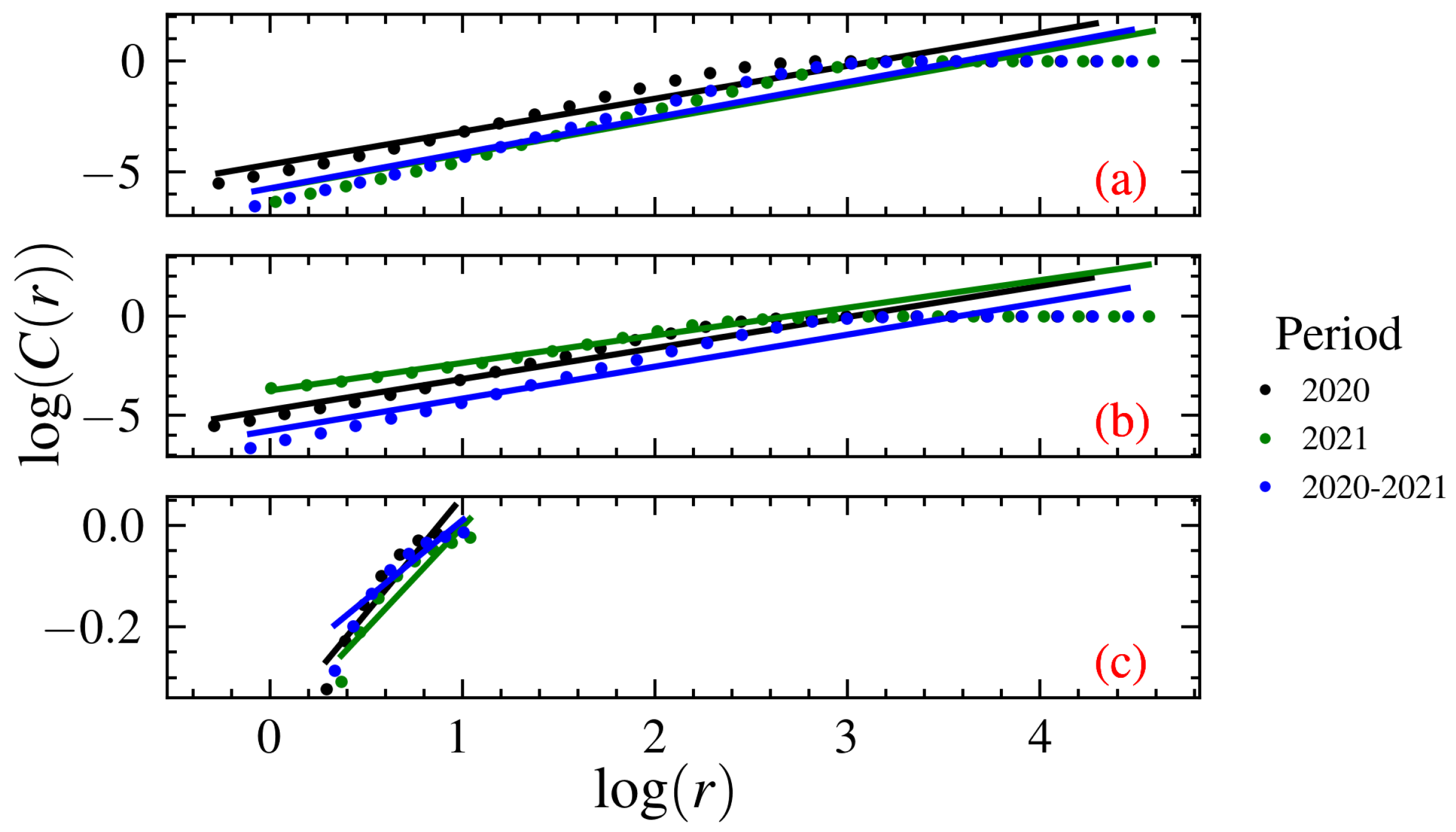
Parameter	Period	m	$\mathit{\tau }$	$\mathit{\lambda }$	${\mathit{d}}_2$
VTEC (Lagos)	2020	11	17	0.031	1.553
VTEC (Lagos)	2021	18	17	0.021	1.775
VTEC (Lagos)	2020–2021	18	17	0.035	1.593
VTEC (Abuja)	2020	11	17	0.011	1.485
VTEC (Abuja)	2021	6	17	0.033	1.388
VTEC (Abuja)	2020–2021	18	17	0.041	1.610
DFS	2020	10	8	−0.010	0.530
DFS	2021	11	10	0.002	0.312
DFS	2020–2021	10	8	−0.009	0.390

. We obtained a time delay value of 17 for VTEC measurements at both Lagos and Abuja. We observed a time delay of 8 for the DFS in 2020 and 2020–2021 and a time delay of 10 in 2021. The time delays observed for other locations include $\tau =40$ for a mid-latitude location during 2001 and 2008 [19] and $\tau =2$ for four months in 2008 at a high-latitude station [47]. The value obtained for VTEC in this study is close to the values of $\tau =16$ reported over the 120° E meridian between 1996 and 2004 [20] and $\tau \ge 18$ reported by [21] at Indian stations of Agatti (geomagnetic latitude 2.38 N), Mumbai (geomagnetic latitude 10.09 N), and Jodhpur (geomagnetic latitude 18.3 N).

The embedding dimension m was also evaluated for the VTEC signals and DFS using the method of false nearest neighbors (Table 1). It was observed that the VTEC values at the two locations had identical embedding dimensions during 2020 and throughout the 2020–2021 period. However, in 2021, Lagos and Abuja obtained values of 18 and 6, respectively. This suggests a significant dynamical variation in 2021 at both locations. The values of embedding dimensions obtained in this study were found to be higher than those reported in other regions of the world [20,21,47]. Variations in location, data considered, dynamics of the study areas, and study methods may account for these differences. The embedding dimensions for the DFS varied between 10 and 11 for the three time periods under consideration.

A positive largest Lyapunov exponent is indicative of chaos in the system. The inverse of the largest Lyapunov exponent is typically used as the system’s predictive horizon. In Figure 8, the linear fit to Equation (7) is shown for both VTEC and DFS. It was observed that the linear fits for the VTEC signals showed positive slopes, which is not obvious in the DFS. The statistics for the fit, which represents the largest Lyapunov exponent, are presented in Table 1. The largest Lyapunov exponent values of 0.031, 0.021, and 0.035 were observed for VTEC in Lagos during the 2020, 2021, and 2020–2021 periods, respectively, while values of 0.011, 0.033, and 0.041 were reported for VTEC in Abuja during the same time period. These values are lower than reported values of 0.3369 [20], 0.22 [23], and 0.1 [22] but higher than 0.0045 [21]. However, they were found to be in the range of 0.023 [47]. A direct consequence of the largest Lyapunov exponent is the prediction horizon for the system, which is the inverse of the Lyapunov exponent. From the results obtained, the prediction horizon for VTEC in Lagos was 32, 48, and 29 h in the periods of 2020, 2021, and 2020–2021, respectively. The prediction horizon in Abuja was estimated to be 90, 30, and 24 h during the periods of 2020, 2021, and 2020–2021, respectively. The Doppler shift frequency in an HF radio signal (DFS) was found to have a negative exponent in 2020 and 2020–2021, while a low positive value (≈0) was obtained for 2021. This suggests that the dynamics of the DFS are not chaotic. It is opined that DFS is a stochastic system. The state of the ionosphere is important, not only for understanding our solar system, but also for various aspects of our existence, including communications and weather systems. A short prediction horizon implies that it is impossible to make long-term predictions about the ionosphere; hence, it reduces our ability to plan for its effect on our communication and weather systems. It also implies that the ionosphere is a dynamic system with rapidly evolving states.

In Figure 9, the slope ($D_2$) of Equation (9) for the parameters is presented with the statistics shown in Table 1. It can be observed that all the parameters observed showed non-integer values of $d_2$. Specifically, $d_2$ was found to be in the range $1.553\le d_2\le 1.775$ in Lagos. Since $d_2$ gives an indication of the number of variables required to model a system, it follows that VTEC in Lagos can be captured as a two-dimensional system. It could be inferred that, due to the closeness of values, the dynamics observed over the 2020–2021 period are driven by the dynamics of the VTEC during 2020. This could also be observed in their respective Lyapunov exponent values. In Abuja, there is a range of $1.388\le d_2\le 1.610$, which implies that the dynamics of the VTEC at this location can be described by two variables. The correlation dimension values obtained in this study were found to be lower than those reported in other studies. Specifically, the estimation of the correlation dimension for the VTEC in other locations across the world yielded values of 2.78 [19], 3.6 [20], 2.74 [21], and 2.8–3.5 [22]. The differences in results could be attributed to our location of choice, period of observation, and length of time for which data were considered.

The dynamics of geospace have been of interest to scientists because of their importance in space infrastructure, satellite communication signals, and terrestrial weather. Several studies have demonstrated that complex structures, not linear regimes, govern activities in different layers of geospace. This is due to the mixing of gases, coupling between different layers, and several driving forces acting differently across the layers of geospace. It has been shown that chaotic dynamics exist in the magnetosphere [18], stratosphere [48], mesosphere [49], and ionosphere [19]. The implication of chaotic dynamics in geospace is that long-term prediction of the system is difficult. The state of the ionosphere is very important due to its huge impact on earth’s satellite radio communications and the attendant effects of satellites domiciled in the region, as well as their associated space-dependent services. The short prediction horizon implies that the predictability of the ionosphere is only guaranteed for a short term. It also implies that the ionosphere is a dynamic system with rapidly evolving states, which requires effective monitoring and periodical forecasting. The results obtained in this study are in agreement with those reported for other regions of the world. We have shown that the ionosphere is a chaotic system at two locations within Nigeria. Our results showed a prediction horizon between 24 and 90 h for the VTEC at the two locations, while at least two variables were needed to describe their dynamics. The change in the DFS of signals as they pass through the ionosphere was also investigated and found to be non-chaotic.

3.3. Linear and Dynamic Coupling

There is a change in the DFS as radio waves propagate through the ionosphere. We employed two approaches, linear and nonlinear, to investigate the relationship between the change in the DFS of a signal originating from one point on earth and its reflection by the ionosphere at another point.

Table 2. Linear and nonlinear relationship between VTEC measurement and DFS at Lagos and Abuja using correlation measures and transfer entropy over different time periods.

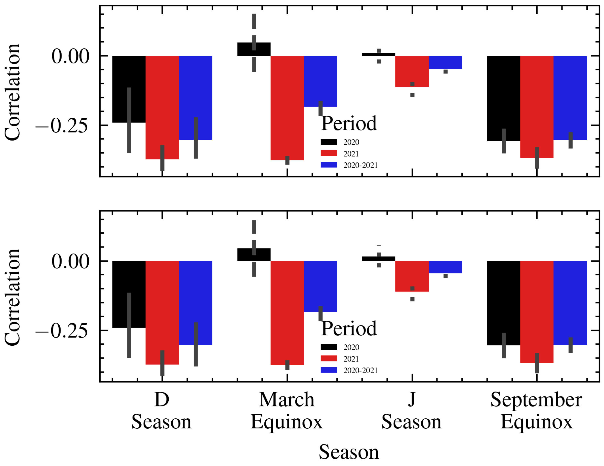
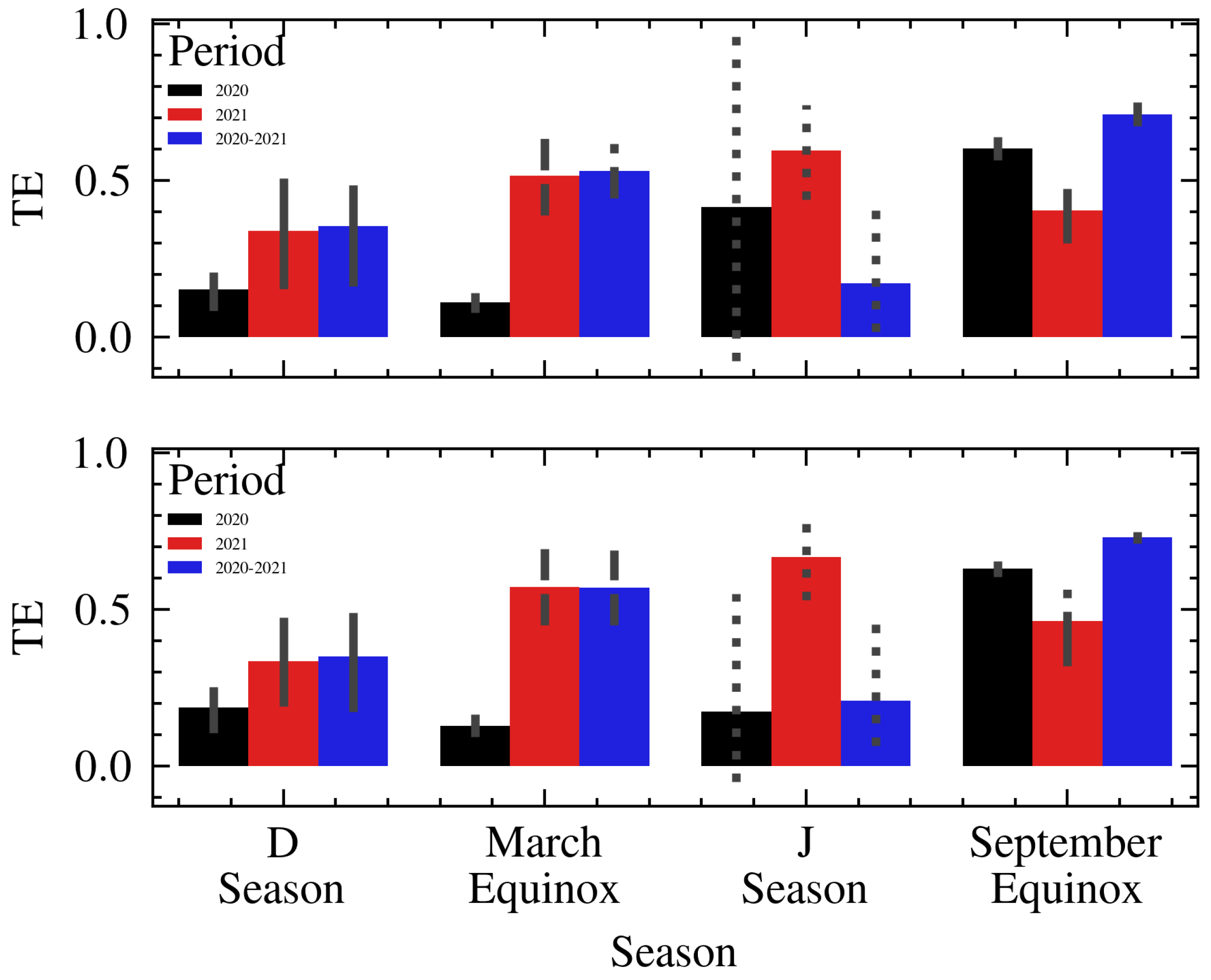
Location	Period	Correlation	TE
Lagos	2020	−0.167	1.073
Lagos	2021	−0.279	0.385
Lagos	2020–2021	−0.219	1.338
Abuja	2020	−0.164	1.114
Abuja	2021	−0.277	0.424
Abuja	2020–2021	−0.216	1.414

shows the statistics for both correlation and transfer entropy measures for different time epochs considered in this study. We observed negative correlations between VTEC measurements and DFS at the two locations under consideration. We found similar correlation values for the two locations. The strongest negative correlation was observed in 2021, while the weakest correlation was reported in 2020. This implies that an increase in ionospheric activity at the two locations corresponds to a decrease in the change in the DFS at the receiving end. A similar analysis was carried out using the nonlinear transfer entropy. Our transfer entropy analysis showed that there was a strong relationship between the VTEC and DFS in 2020–2021 compared to the other two time frames. Across the years, a stronger connection was observed between VTEC and DFS in 2020 compared to 2021 in the two locations. Also, values of transfer entropy were found to be higher in Abuja compared to Lagos, whereas the correlation coefficient was slightly higher in Lagos compared to Abuja. While the values of transfer entropies were close in the two locations, there were sufficient differences to discriminate the coupling, which was not obvious in the correlation analysis. The year 2020, with a mean sunspot number (Rz) of 8.8, had a stronger transfer entropy than 2021, a year with high solar activity (Rz = 29.6).

The relationship between VTEC and DFS was also considered on a monthly scale using the correlation (Figure 10 and Figure 11) and transfer entropy (Figure 12 and Figure 13) at the two locations. In Figure 10, correlation values showed a weaker relationship between VTEC and DFS during the months of April to August for the periods 2020, 2021, and 2020–2021. The values were largely negative at the two locations, except in the month of April, where a positive value was obtained. Furthermore, Figure 11 and Figure 13, respectively, show the seasonal variation in the correlation values and transfer entropy between the VTEC and DFS. The summer (June) solstice has a higher correlation than the other seasons. This shows that an increase in ionospheric activity corresponds to a decrease in the DFS. The correlation was observed to be stronger in the year with higher solar activity (2021), but weaker in 2020. Replicating the analysis using transfer entropy yielded another scenario, as presented in Figure 11 and Figure 12. The influence of VTEC on DFS was different in 2020 compared to 2021 in both Lagos and Abuja. In 2020, there was little or no influence in most months of the year except June (Abuja), July (Lagos), September, and October. Figure 11 shows that the DFS of the propagated radio signal is more impacted by variability in the ionosphere, as captured by the VTEC in the solstitial months of June/July at Abuja/Lagos and the September equinox at the two locations. The seasonal effects in the ionospheric processes have been discussed by several authors using different parameters and techniques; see, for example, [31] and the references therein. Generally, the influence was weaker in 2020 compared to the other two periods under consideration in both Lagos and Abuja. In 2021 and 2020–2021, there was an identical increase in influence at both locations from January to April. Beyond April 2020 and May 2021, the influence declined towards December. It can be inferred from the correlation and transfer entropy analysis that the VTEC has little or no influence on the DFS in the months of May through July during the combined period of 2020–2021.

The linear relationship between VTEC and DFS measurements suggests that an increase in VTEC will cause a decrease in DFS measurements. When there is an increase in the total electron content within the ionosphere, there are more electrons for the signals to interact with. This interaction causes the degradation of signals. However, the correlation analysis does not suggest direct causality between the VTEC and DFS. The transfer entropy provided a conclusive argument that changes in VTEC cause significant changes in DFS. By exploring the probability distribution space of both variables, it was concluded that changes in VTEC cause changes in DFS.

4. Conclusions

Chaos theory has evolved over the past few decades due to improved techniques, the robustness of its processes, and the application of the results. There have only been a few attempts to apply chaos theory to the study of the ionosphere. This study extends the work of previous authors by considering two tropical locations close to the equator over a period of two years in relation to the quality of the HF radio signals transmitted between the two study areas. Our results showed that the VTEC at the two locations had the same embedding dimension in both locations for all the periods under consideration. Using both Lyapunov exponent and correlation dimension measures, we conclude that the dynamics of the VTEC at the two locations are chaotic in nature. However, the signal quality between these two locations was found to be a stochastic process. The influence of the ionosphere on propagated HF radio signals between the two locations was investigated using transfer entropy and correlation analysis. A negative correlation was observed at the beginning of the year, which weakened during the middle of the year, predominantly during the June solstice, before returning to a negative correlation towards the end of the year. The use of correlation measures in this study is for comparison with other nonlinear measures while taking into consideration the strength of the correlation values. Our discussion highlights the weakness of the correlation values themselves. However, the transfer entropy analysis revealed a weak nonlinear relationship between the two variables in January. This increased to a peak in April during the 2021 and 2020–2021 periods. Transfer entropy provides direct evidence that the VTEC influences radio signals in the ionosphere. This causality was observed to change during different months of the year. This means that when there are changes in the ionosphere, there is a corresponding change in the signal that passes through it. Thus, the state of the ionosphere is important for radio communication. The observed linear and nonlinear relationships between the ionosphere and signal quality at the two locations can be incorporated into communication planning for high-frequency radio systems at both annual and monthly scales. This study can be extended to other regions, especially high-latitude stations. Furthermore, the relationships at smaller temporal scales can be explored. There are other nonlinear techniques that can reveal more features of the VTEC that can be considered in future studies.

References

- Heelis, R.; Maute, A. Challenges to understanding the Earth’s ionosphere and thermosphere. J. Geophys. Res. Space Phys. 2020, 125, e2019JA027497. [Google Scholar] [CrossRef]
- Ogunjo, S.; Dada, J.; Oluyamo, S.; Fuwape, I. Tropospheric delay in microwave propagation in Nigeria. Arab. J. Geosci. 2021, 14, 1542. [Google Scholar] [CrossRef]
- Yiğit, E.; Knížová, P.K.; Georgieva, K.; Ward, W. A review of vertical coupling in the Atmosphere–Ionosphere system: Effects of waves, sudden stratospheric warmings, space weather, and of solar activity. J. Atmos. Sol.-Terr. Phys. 2016, 141, 1–12. [Google Scholar] [CrossRef]
- Mukherjee, S.; Sarkar, S.; Purohit, P.; Gwal, A. Seasonal variation of total electron content at crest of equatorial anomaly station during low solar activity conditions. Adv. Space Res. 2010, 46, 291–295. [Google Scholar] [CrossRef]
- Abdullah, M.; Strangeways, H.J.; Walsh, D.M. Improving ambiguity resolution rate with an accurate ionospheric differential correction. J. Navig. 2009, 62, 151–166. [Google Scholar] [CrossRef]
- Reznychenko, A.I.; Koloskov, A.V.; Sopin, A.O.; Yampolski, Y.M. Statistic of seasonal and diurnal variations of Doppler frequency shift of hf signals at mid-latitude radio path. Radio Phys. Radio Astron. 2020, 25, 118–135. [Google Scholar] [CrossRef]
- Boldovskaya, I. Doppler frequency shifts of radio waves reflected by parabolic and quasi-parabolic ionospheric layers. J. Atmos. Terr. Phys. 1982, 44, 305–311. [Google Scholar] [CrossRef]
- Liu, J.; Chiu, C.; Lin, C. The solar flare radiation responsible for sudden frequency deviation and geomagnetic fluctuation. J. Geophys. Res. Space Phys. 1996, 101, 10855–10862. [Google Scholar] [CrossRef]
- Chum, J.; Šindelářová, T.; Laštovička, J.; Hruška, F.; Burešová, D.; Baše, J. Horizontal velocities and propagation directions of gravity waves in the ionosphere over the Czech Republic. J. Geophys. Res. Space Phys. 2010, 115. [Google Scholar] [CrossRef]
- Chum, J.; Liu, J.Y.; Chen, S.P.; Cabrera, M.A.; Laštovička, J.; Baše, J.; Burešová, D.; Fišer, J.; Hruška, F.; Ezquer, R. Spread F occurrence and drift under the crest of the equatorial ionization anomaly from continuous Doppler sounding and FORMOSAT-3/COSMIC scintillation data. Earth Planets Space 2016, 68, 56. [Google Scholar] [CrossRef]
- Nishioka, M.; Tsugawa, T.; Kubota, M.; Ishii, M. Concentric waves and short-period oscillations observed in the ionosphere after the 2013 Moore EF5 tornado. Geophys. Res. Lett. 2013, 40, 5581–5586. [Google Scholar] [CrossRef]
- Chum, J.; Diendorfer, G.; Šindelářová, T.; Baše, J.; Hruška, F. Infrasound pulses from lightning and electrostatic field changes: Observation and discussion. J. Geophys. Res. Atmos. 2013, 118, 10–653. [Google Scholar] [CrossRef]
- Sindelarova, T.; Chum, J.; Skripnikova, K.; Base, J. Atmospheric infrasound observed during intense convective storms on 9–10 July 2011. J. Atmos. Sol.-Terr. Phys. 2015, 122, 66–74. [Google Scholar] [CrossRef]
- López-Urias, C.; Vazquez-Becerra, G.E.; Nayak, K.; López-Montes, R. Analysis of Ionospheric Disturbances during X-Class Solar Flares (2021–2022) Using GNSS Data and Wavelet Analysis. Remote Sens. 2023, 15, 4626. [Google Scholar] [CrossRef]
- Sergeeva, M.A.; Maltseva, O.A.; Vesnin, A.M.; Blagoveshchensky, D.V.; Gatica-Acevedo, V.J.; Gonzalez-Esparza, J.A.; Chernov, A.G.; Orrala-Legorreta, I.D.; Melgarejo-Morales, A.; Gonzalez, L.X.; et al. Solar Flare Effects Observed over Mexico during 30–31 March 2022. Remote Sens. 2023, 15, 397. [Google Scholar] [CrossRef]
- Salikhov, N.; Shepetov, A.; Pak, G.; Saveliev, V.; Nurakynov, S.; Ryabov, V.; Zhukov, V. Disturbances of Doppler Frequency Shift of Ionospheric Signal and of Telluric Current Caused by Atmospheric Waves from Explosive Eruption of Hunga Tonga Volcano on January 15, 2022. Atmosphere 2023, 14, 245. [Google Scholar] [CrossRef]
- Strogatz, S.H. Nonlinear Dynamics and Chaos: Lab Demonstrations; Internet-First University Press: Ithaca, NY, USA, 1994. [Google Scholar]
- Ogunjo, S.T.; Rabiu, A.B.; Fuwape, I.A.; Obafaye, A.A. Evolution of Dynamical Complexities in Geospace as Captured by Dst Over Four Solar Cycles 1964–2008. J. Geophys. Res. Space Phys. 2021, 126, e2020JA027873. [Google Scholar] [CrossRef]
- Materassi, M.; Alberti, T.; Migoya-Orué, Y.; Radicella, S.M.; Consolini, G. Chaos and Predictability in Ionospheric Time Series. Entropy 2023, 25, 368. [Google Scholar] [CrossRef] [PubMed]
- Ke, X.; Wan, W.X.; Ning, B.Q. Chaotic Properties Analysis and Nonlinear Prediction of Ionospheric Total Electron Content over 120° E Magnetism Equator. Chin. J. Geophys. 2006, 49, 1130–1138. [Google Scholar]
- Unnikrishnan, K. A comparative study on chaoticity of equatorial/low latitude ionosphere over Indian subcontinent during geomagnetically quiet and disturbed periods. Nonlinear Process. Geophys. 2010, 17, 765–776. [Google Scholar] [CrossRef]
- Ogunsua, B.; Laoye, J.; Fuwape, I.; Rabiu, A. The comparative study of chaoticity and dynamical complexity of the low-latitude ionosphere, over Nigeria, during quiet and disturbed days. Nonlinear Process. Geophys. 2014, 21, 127–142. [Google Scholar] [CrossRef]
- Ogunsua, B. Low latitude ionospheric TEC responses to dynamical complexity quantifiers during transient events over Nigeria. Adv. Space Res. 2018, 61, 1689–1701. [Google Scholar] [CrossRef]
- Ogunjo, S.T.; Fuwape, I.A. Nonlinear characterization and interaction in teleconnection patterns. Adv. Space Res. 2020, 65, 2723–2732. [Google Scholar] [CrossRef]
- Kantz, H.; Schreiber, T. Nonlinear Time Series Analysis; Cambridge University Press: Singapore, 2004; Volume 7. [Google Scholar]
- Fuwape, I.A.; Ogunjo, S.T.; Dada, J.B.; Ashidi, G.A.; Emmanuel, I. Phase synchronization between tropospheric radio refractivity and rainfall amount in a tropical region. J. Atmos. Sol.-Terr. Phys. 2016, 149, 46–51. [Google Scholar] [CrossRef]
- Olusola, A.; Ogunjo, S.; Olusegun, C. The role of teleconnections and solar activity on the discharge of tropical river systems within the Niger basin. Environ. Monit. Assess. 2023, 195, 476. [Google Scholar] [CrossRef] [PubMed]
- Rabiu, A.B.; Mamukuyomi, A.; Joshua, E. Variability of equatorial ionosphere inferred from geomagnetic field measurements. Bull. Astron. Soc. India 2007, 35. [Google Scholar]
- Olugbon, B.; Oyeyemi, E.; Kascheyev, A.; Rabiu, A.; Obafaye, A.; Odeyemi, O.; Adewale, A. Daytime equatorial spread F-like irregularities detected by HF Doppler receiver and digisonde. Space Weather 2021, 19, e2020SW002676. [Google Scholar] [CrossRef]
- Chum, J.; Urbář, J.; Laštovička, J.; Cabrera, M.A.; Liu, J.Y.; Bonomi, F.A.M.; Fagre, M.; Fišer, J.; Mošna, Z. Continuous Doppler sounding of the ionosphere during solar flares. Earth Planets Space 2018, 70, 198. [Google Scholar] [CrossRef]
- Eyelade, V.A.; Adewale, A.O.; Akala, A.O.; Bolaji, O.S.; Rabiu, A.B. Studying the variability in the diurnal and seasonal variations in GPS total electron content over Nigeria. Ann. Geophys. 2017, 35, 701–710. [Google Scholar] [CrossRef]
- Takens, F. Detecting strange attractors in turbulence. In Dynamical Systems and Turbulence, Warwick 1980; Springer: Berlin/Heidelberg, Germany, 1981; pp. 366–381. [Google Scholar]
- Fraser, A.M.; Swinney, H.L. Independent coordinates for strange attractors from mutual information. Phys. Rev. A 1986, 33, 1134. [Google Scholar] [CrossRef]
- Kennel, M.B.; Brown, R.; Abarbanel, H.D. Determining embedding dimension for phase-space reconstruction using a geometrical construction. Phys. Rev. A 1992, 45, 3403. [Google Scholar] [CrossRef] [PubMed]
- Rosenstein, M.T.; Collins, J.J.; De Luca, C.J. A practical method for calculating largest Lyapunov exponents from small data sets. Phys. D Nonlinear Phenom. 1993, 65, 117–134. [Google Scholar] [CrossRef]
- Grassberger, P.; Procaccia, I. Characterization of strange attractors. Phys. Rev. Lett. 1983, 50, 346. [Google Scholar] [CrossRef]
- Ma, J. Estimating transfer entropy via copula entropy. arXiv 2019, arXiv:1910.04375. [Google Scholar]
- Mannucci, A.J.; Wilson, B.D.; Edwards, C.D. A new method for monitoring the Earth’s ionospheric total electron content using the GPS global network. In Proceedings of the P6th International Technical Meeting of the Satellite Division of the Institute of Navigation (ION GPS 1993), Salt Lake City, UT, USA, 22–24 September 1993; pp. 1323–1332. [Google Scholar]
- Wielgosz, P.; Milanowska, B.; Krypiak-Gregorczyk, A.; Jarmołowski, W. Validation of GNSS-derived global ionosphere maps for different solar activity levels: Case studies for years 2014 and 2018. GPS Solut. 2021, 25, 103. [Google Scholar] [CrossRef]
- Okoh, D.; Seemala, G.; Rabiu, B.; Habarulema, J.B.; Jin, S.; Shiokawa, K.; Otsuka, Y.; Aggarwal, M.; Uwamahoro, J.; Mungufeni, P.; et al. A neural network-based ionospheric model over Africa from Constellation Observing System for Meteorology, Ionosphere, and Climate and Ground Global Positioning System observations. J. Geophys. Res. Space Phys. 2019, 124, 10512–10532. [Google Scholar] [CrossRef]
- Obrou, O.; Mene, M.; Kobea, A.; Zaka, K. Equatorial total electron content (TEC) at low and high solar activity. Adv. Space Res. 2009, 43, 1757–1761. [Google Scholar] [CrossRef]
- Bagiya, M.S.; Joshi, H.; Iyer, K.; Aggarwal, M.; Ravindran, S.; Pathan, B. TEC variations during low solar activity period (2005–2007) near the equatorial ionospheric anomaly crest region in India. Ann. Geophys. 2009, 27, 1047–1057. [Google Scholar] [CrossRef]
- Titheridge, J. Changes in atmospheric composition inferred from ionospheric production rates. J. Atmos. Terr. Phys. 1974, 36, 1249–1257. [Google Scholar] [CrossRef]
- Wu, C.C.; Fry, C.; Liu, J.Y.; Liou, K.; Tseng, C.L. Annual TEC variation in the equatorial anomaly region during the solar minimum: September 1996–August 1997. J. Atmos. Sol.-Terr. Phys. 2004, 66, 199–207. [Google Scholar] [CrossRef]
- Rama Rao, P.; Gopi Krishna, S.; Niranjan, K.; Prasad, D. Temporal and spatial variations in TEC using simultaneous measurements from the Indian GPS network of receivers during the low solar activity period of 2004–2005. Ann. Geophys. 2006, 24, 3279–3292. [Google Scholar] [CrossRef]
- Rishbeth, H.; Müller-Wodarg, I.; Zou, L.; Fuller-Rowell, T.; Millward, G.; Moffett, R.; Idenden, D.; Aylward, A. Annual and semiannual variations in the ionospheric F2-layer: II. Physical discussion. Ann. Geophys. 2000, 18, 945–956. [Google Scholar] [CrossRef]
- Shuhui, L.; Junhuan, P. Ionospheric TEC prediction and analysis based on phase space reconstruction. In Proceedings of the 2010 International Conference on Mechanic Automation and Control Engineering, Wuhan, China, 26–28 June 2010; IEEE: Piscataway, NJ, USA, 2010; pp. 1936–1939. [Google Scholar]
- Ngan, K.; Shepherd, T.G. A closer look at chaotic advection in the stratosphere. Part II: Statistical diagnostics. J. Atmos. Sci. 1999, 56, 4153–4166. [Google Scholar] [CrossRef]
- Sonnemann, G.; Fichtelmann, B. Subharmonics, cascades of period doubling, and chaotic behavior of photochemistry of the mesopause region. J. Geophys. Res. Atmos. 1997, 102, 1193–1203. [Google Scholar] [CrossRef]