Computational Fluid Dynamics Simulation of High-Resolution Spatial Distribution of Sensible Heat Fluxes in Building-Congested Area

Abstract

Urban areas consist of various land cover types, with a high proportion of artificial surfaces among them. This leads to unfavorable thermal environments in urban areas. Continuous research on the thermal environment, specifically on the sensible heat flux (Q_h), has been conducted. However, previous research has faced temporal, spatial, and resolution limitations when it comes to detailed analysis of sensible heat flux in urban areas. Therefore, in this study, a computational fluid dynamics (CFD) model combined with the LDAPS and the VUCM was developed to simulate Q_h at one-hour intervals over a 1-month period in an urban area with various land cover types. Model validation was performed by comparing it with measurements, confirming the suitability of the model for simulating Q_h. The land cover was categorized into five types: building, road, bare land, grassland, and tree areas. Q_h exhibited distinct patterns depending on the land cover type. When averaging the Q_h distribution over the target period, buildings, roads, and bare land areas showed a predominance of upward Q_h values, while grassland and tree areas displayed dominant downward Q_h values. Additionally, even within the same land cover types, slight Q_h variations were identified based on their surroundings. The averaged Q_h value for building areas was the highest at 36.79 W m⁻², while that for tree areas was −3.04 W m⁻². Moreover, during the target period, the time-averaged Q_h showed that building, road, and bare land areas peaked at 14 LST, while grassland and tree areas exhibited very low Q_h values. Notably, buildings reached a maximum Q_h of 103.30 W m⁻² but dropped to a minimum of 1.14 W m⁻² at 5 LST.

1. Introduction

Urban areas are composed of various land covers, including buildings, roads, forests, grasslands, and water systems. Land covers such as concrete and asphalt, which occupy a significant portion of cities, absorb more solar radiation energy than natural vegetation, leading to relatively high temperatures [1]. Sensible heat fluxes from the land surface increase as urban redevelopment increases the proportion of land cover such as concrete and asphalt and increases fossil fuel consumption and artificial heat emissions [2]. An increased sensible heat flux enhances the instability of the lower atmosphere, which not only affects precipitation in urban areas [3], but also worsens thermal comfort for pedestrians [4].

Continuous studies are being conducted on sensible heat flux analysis to investigate the thermal environment in urban areas. Previous research suggests that adopting optimal roof designs on buildings can help mitigate urban heat islands, as the sensible heat flux is influenced by the color, shape, and material of building roofs [5,6,7]. Additionally, tree planting and building albedo also impact sensible heat fluxes [8,9]. Studies on sensible heat fluxes are mostly conducted using field measurements or remote sensing [1,10,11,12,13,14,15]. However, the spatial resolution of these observations is not sufficient to provide a comprehensive understanding of the spatiotemporal variability of the sensible heat flux in urban areas. Even numerical weather prediction models lack the necessary resolution to fully capture these phenomena. Therefore, to fully understand the effects of sensible heat flux and air temperatures on different land cover types, it is necessary to use numerical models that can resolve buildings and take into account surface heating on different land covers. To the best of our knowledge, there have been few studies that have focused on the analysis of the spatial distribution of sensible heat fluxes, taking into consideration both buildings and land cover types in urban areas [16,17].

Computational fluid dynamics (CFD) models have been widely applied in simulating urban- or small-scale atmospheric phenomena, because they can resolve buildings and small terrains that act as essential external forcings in the formation of airflow within urban canopy layers [18,19,20,21,22,23,24,25,26,27]. Antoniou et al. [18] utilized a CFD model to simulate the wind and temperature in urban areas that are densely populated with low-rise buildings and validated the results using field measurement data. Discrepancies between the model and measurements were attributed to factors such as the diversity of materials used in urban construction, the simplification of various building forms, the exclusion of trees and green fields, and the inherent limitations of the model. Zhang et al. [19] utilized an LES-based CFD model to assess air ventilation in real urban areas by employing twisted wind profiles, which occur in hilly terrains, as inlet conditions for the CFD model. It is recommended to use twisted wind profiles as inlet conditions when assessing air ventilation in actual urban areas. Brozovsky et al. [20,21] developed a CFD model that incorporates the thermal effects of evapotranspiration from trees and grass, which was validated using measurement data. This model was applied to analyze the building energy demand, which was influenced by different types of urban surfaces in high-rise buildings located within a university campus. The analysis indicated that green spaces can reduce the energy demand and enhance indoor thermal comfort during the summer months. Moradpour et al. [22] used a CFD model to investigate the impact of green spaces near highways on urban air quality by setting various conditions for wind direction, leaf area density, and background concentration. The study found that green spaces reduced the average concentrations of PM₁₀, CO, NO_x, and VOC at pedestrian levels, with reduction rates varying based on the wind direction and species. Lee et al. [23] used a model that integrates the chemical mechanism of the global 3-D chemical transport model (GEOS-Chem) into a CFD model to analyze the air quality in urban areas. This model was utilized to investigate the impact of heating on the dispersion of secondary inorganic aerosols in an urban street canyon. The study found that heating reduced the concentration of secondary inorganic aerosols, with the heating effects varying depending on the aerosol species. Maggiotto et al. [24] compared the predictive performance of a CFD model and a temperature perturbation-type model for forecasting urban temperatures. Both models reasonably simulated the diurnal variation of temperature when compared with measurements. The CFD model was found to be suitable for analyzing the flow patterns and temperature distribution around buildings and vegetation, while the perturbation-type model was deemed appropriate for predicting and evaluating the urban thermal environment. Huang et al. [25] and Ashie and Kono [26] assessed the urban thermal environment by applying various input data to a CFD model, including anthropogenic heat, calculated by estimating the sensible and latent heat emitted from buildings, radiation analysis, heat conduction analysis, and other factors. Ashie and Kono [26] reported that reducing the area that is occupied by buildings increases the regions where the temperature decreases. Allegrini et al. [27] used a CFD model combined with building energy simulations to analyze heat flux across six types of urban morphology, finding that most of the heat escapes in the top and downstream directions of urban areas. Research using CFD models is actively pursued on subjects such as wind, temperature, and air quality, and studies to analyze the thermal environment of urban areas with CFD models are progressing. Additionally, many studies have combined CFD models with other models and validated their performance using measurement data. However, studies that spatially analyze various land covers in actual urban areas are scarce, and research on sensible heat flux, a critical component for analyzing thermal environments, has been very limited.

This study developed a high-resolution method for estimating the sensible heat flux in building-congested areas with various land cover types. This method is based on CFD models and coupled with a vegetation urban canopy model [28] and the local data assimilation and prediction system (LDAPS) operated by the Korean Meteorological Administration (LDAPS-CFD-VUCM). Using the developed high-resolution sensible heat flux estimation method, the sensible heat flux was estimated over a one-month period for areas in Seoul, South Korea, characterized by diverse land cover types and dense buildings. The estimation was conducted at a grid resolution of 10 m horizontally and 2 m vertically. The estimated sensible heat flux was validated using wind, temperature, and sensible heat flux measurements from flux towers located within the target area, and the spatial distribution of the sensible heat flux was analyzed by land cover type and time.

2. Methodology

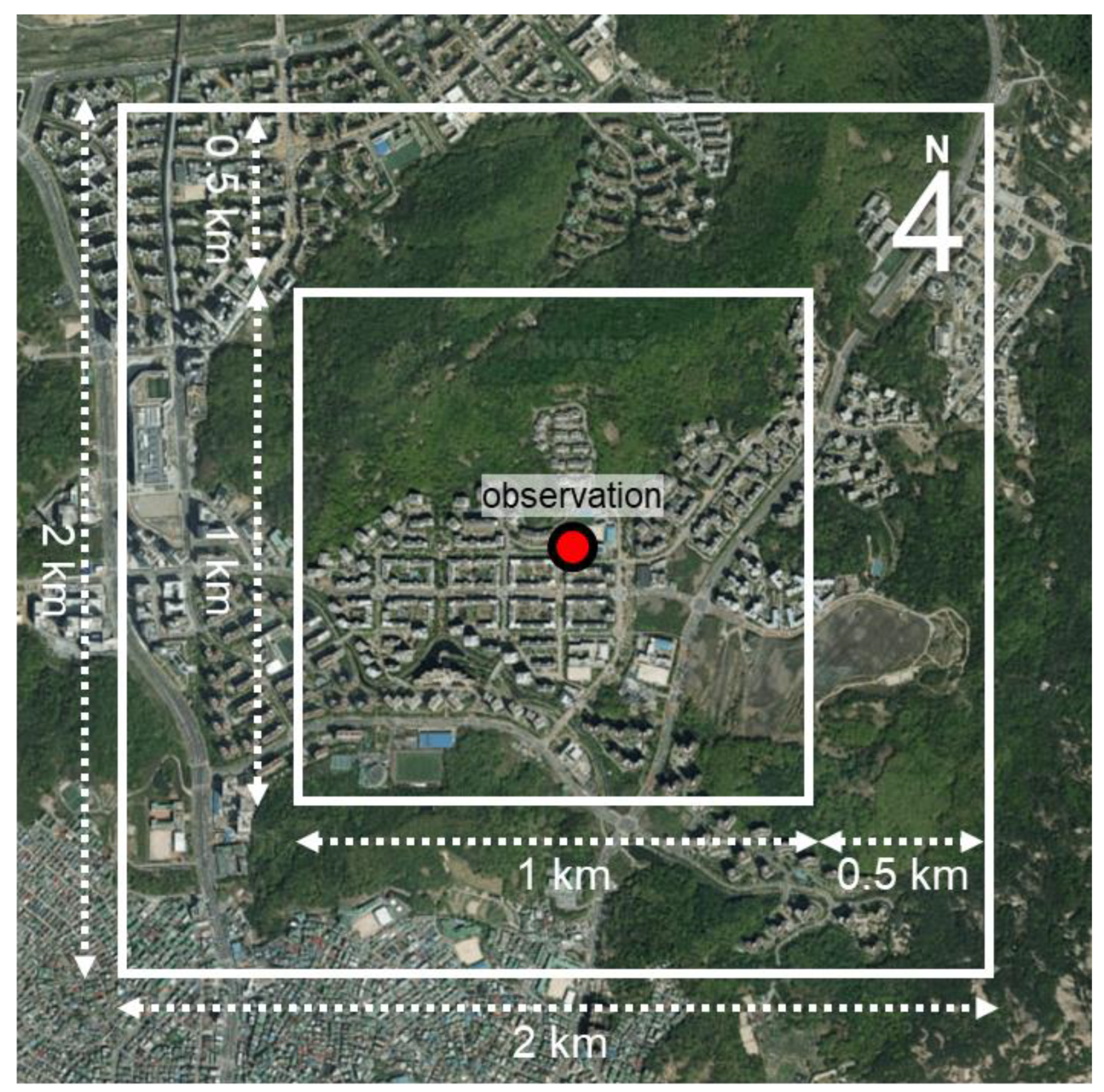
2.1. Target Area and Period

The target area considered in this study is a 1 km by 1 km area, with the center located at 37.6350° N and 126.9287° E (Figure 1). The area is located in Eunpyeong-gu, Seoul, and characterized as a building-congested zone. Predominantly, the buildings in the target area are residential, with some commercial facilities and schools also present. Buildings in the center of the area are typically low-rise, with seven stories or less. Taller buildings, with ten stories or more, are generally found at the edges of the area. The majority of roads in the area are located around buildings, and areas without buildings or roads are primarily grassland. To the north of the target area is a mountain reaching 132.7 m above sea level, and to the east is undeveloped bare land. A narrow stream runs in an east–west direction in the south, but it contains very little water and is surrounded by dense vegetation. Thus, in this study, streams were considered to be grasslands. Overall, the target area encompasses various land cover types, including buildings (10.02%), roads (27.93%), bare land (11.02%), trees (31.82%), and grasslands (18.44%). The target period was from 1 September to 30 September 2014, during which sensible heat flux (Q_h) measurements were taken.

2.2. Measurement Data

To validate the simulation results, wind speeds, wind directions, air temperatures, and Q_h measured at a flux tower from 1 September to 30 September 2014 were used. This tower, 10 m tall, is equipped with a three-dimensional sonic anemometer (CSAT3 from Campbell Scientific, Inc., Logan, UT, USA) and is installed on the rooftop of a 20 m high building located at the center of the target area (the red dot in Figure 1). The measurements were conducted at a 10 Hz sampling rate, and Q_h was calculated using a 30 min averaging period. Detailed information about the measurements is available in [2].

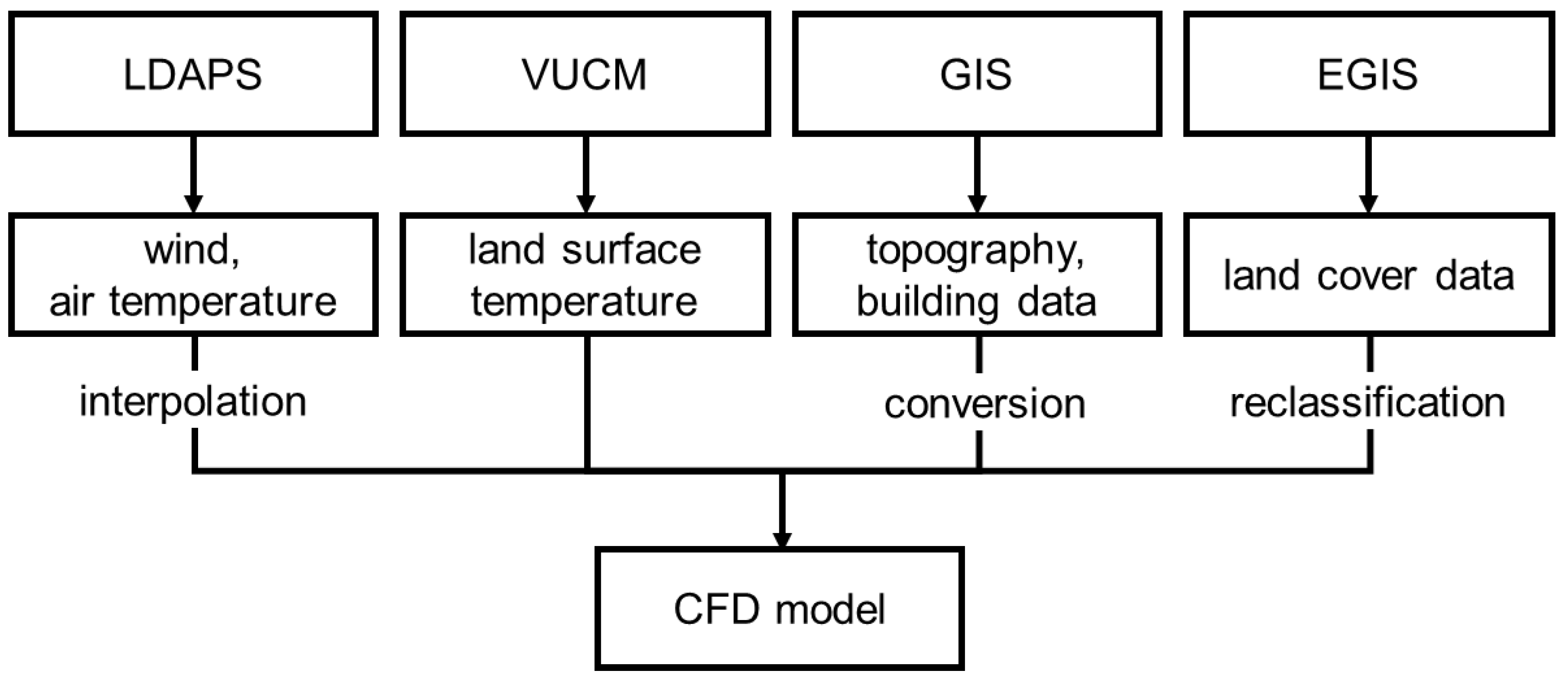
2.3. Numerical Models

The CFD model used in this study solves the unsteady (time-dependent) Reynolds-averaged Navier–Stokes (RANS) equations on a staggered grid system, using the finite volume method and the SIMPLE (semi-implicit method for the pressure-linked equation) algorithm [29]. The model assumes a three-dimensional, non-hydrostatic, and Boussinesq airflow system and employs the renormalization group (RNG) k-ε turbulence closure scheme for turbulence parameterization [30]. To account for the effects of the turbulent boundary layer near solid wall surfaces like buildings, the wall boundary conditions proposed by Versteeg and Malalasekera [31] were implemented.

The momentum and mass conservation equations, thermodynamic energy equation can be expressed as follows:

$$\frac{\partial U_i}{\partial t}+U_j\frac{\partial U_i}{\partial x_j}=-\frac{1}{{\rho }_0}\frac{\partial P^{*}}{\partial x_i}+{\delta }_{i3}g\frac{T^{*}}{T_0}+\mathsf{\nu }\frac{{\partial }^2{U}_i}{\partial x_j\partial x_j}-\frac{\partial }{\partial x_j}\left(\overline{u_i{u}_j}\right)$$

(1)

$$\frac{\partial U_i}{\partial x_j}=0$$

(2)

$$\frac{\partial T}{\partial t}+U_j\frac{\partial T}{\partial x_j}=\kappa \frac{{\partial }^{2}T}{\partial x_j\partial x_j}-\frac{\partial }{\partial x_j}\left(\overline{T^{’}{u}_j}\right)+S_h$$

(3)

where $x_i$, $U_i$, and $u_i$ indicate the $i^{th}$ Cartesian coordinate (i = 1, 2, 3), the $i^{th}$ mean velocity component, and the fluctuation in the $i^{th}$ mean velocity component, respectively. $t$, $P^{*}$, ${\rho }_0$ and ${\delta }_{ij}$ are the time, deviation of pressure from the reference value, air density and the Kronecker delta, respectively. $\mathsf{\nu }$ and $\kappa$ are the kinematic viscosity, thermal diffusivity of air, respectively. $\mathrm{g}$, $T$, $T^{’}$, $T_0$, $T^{*}$ and $S_h$ indicate the acceleration due to gravity, mean temperature, fluctuation from $T$, reference temperature, deviation of temperature from its reference value and the source/sink term of heat, respectively. The Reynolds stresses in Equation (1) are parameterized as follows:

$$-\overline{u_i{u}_j}={\nu }_t\left(\frac{\partial U_i}{\partial x_j}+\frac{\partial U_j}{\partial x_i}\right)-\frac{2}{3}{\delta }_{ij}k$$

(4)

$$-\overline{T^{’}{u}_j}={\kappa }_t\frac{\partial T}{\partial x_j}$$

(5)

where ${\nu }_t$, ${\kappa }_t$ and $k$ are the turbulent diffusivities of momentum, heat, and turbulent kinetic energy (TKE), respectively. The ${\nu }_t$ is calculated based on the TKE and its dissipation rate ($\epsilon$) as follow;

$${\nu }_t=C_{\mu }\frac{k^2}{\epsilon }$$

(6)

where $C_{\mu }$ is an empirical constant. The prognostic equations of the TKE and $\epsilon$ in the RNG k-ε turbulence closure scheme can be expressed as follows:

$$\frac{\partial k}{\partial t}+U_j\frac{\partial k}{\partial x_j}=-\overline{u_i{u}_j}\frac{\partial U_i}{\partial x_j}+\frac{{\delta }_{3j}g}{T_0}\overline{T^{’}{u}_j}+\frac{\partial }{\partial x_j}\left(\frac{{\nu }_t}{{\sigma }_k}\frac{\partial k}{\partial x_j}\right)-\epsilon$$

(7)

$$\frac{\partial \epsilon }{\partial t}+U_j\frac{\partial \epsilon }{\partial x_j}=-C_{\epsilon 1}\frac{\epsilon }{k}\overline{u_i{u}_j}\frac{\partial U_i}{\partial x_j}+C_{\epsilon 1}\frac{\epsilon }{k}\frac{{\delta }_{3j}g}{T_0}\overline{T^{’}{u}_j}+\frac{\partial }{\partial x_j}\left(\frac{{\nu }_t}{{\sigma }_{\epsilon }}\frac{\partial \epsilon }{\partial x_j}\right)-C_{\epsilon 2}\frac{{\epsilon }^2}{k}-R$$

(8)

where R is a strain rate term given as

$$R=\frac{C_{\mu }{\eta }^3\left(1-\eta /{\eta }_0\right){\epsilon }^2}{\left(1+{\beta }_0{\eta }^3\right)k}$$

(9)

$$\eta =\frac{k}{\epsilon }{\left[\left(\frac{\partial U_i}{\partial x_j}+\frac{\partial U_j}{\partial x_i}\right)\frac{\partial U_i}{\partial x_j}\right]}^{1/2}$$

(10)

where $C_{\mu }$, $C_{\epsilon 1}$, $C_{\epsilon 2}$, ${\mathsf{\sigma }}_k$, ${\mathsf{\sigma }}_{\mathsf{\epsilon }}$, ${\eta }_0$, and ${\beta }_0$ are empirical constants specified as follows:

$$\left(C_{\mu },C_{\epsilon 1},C_{\epsilon 2},{\mathsf{\sigma }}_k,{\mathsf{\sigma }}_{\mathsf{\epsilon }},{{\eta }_0,\beta }_0\right)=\left(0.0845,1.42,1.68,0.7179,0.7179,4.377,0.012\right)$$

(11)

The model has been extensively validated against various experimental wind tunnel results [32,33,34,35,36] and has been widely applied to simulate flows and dispersions around a single street canyon [37,38], a group of buildings [32,33,34], and building-congested areas [35,39,40]. A more detailed description of the CFD model can be found in [32]. The governing equation set is numerically integrated up to 3600 s, with a time step of 1 s.

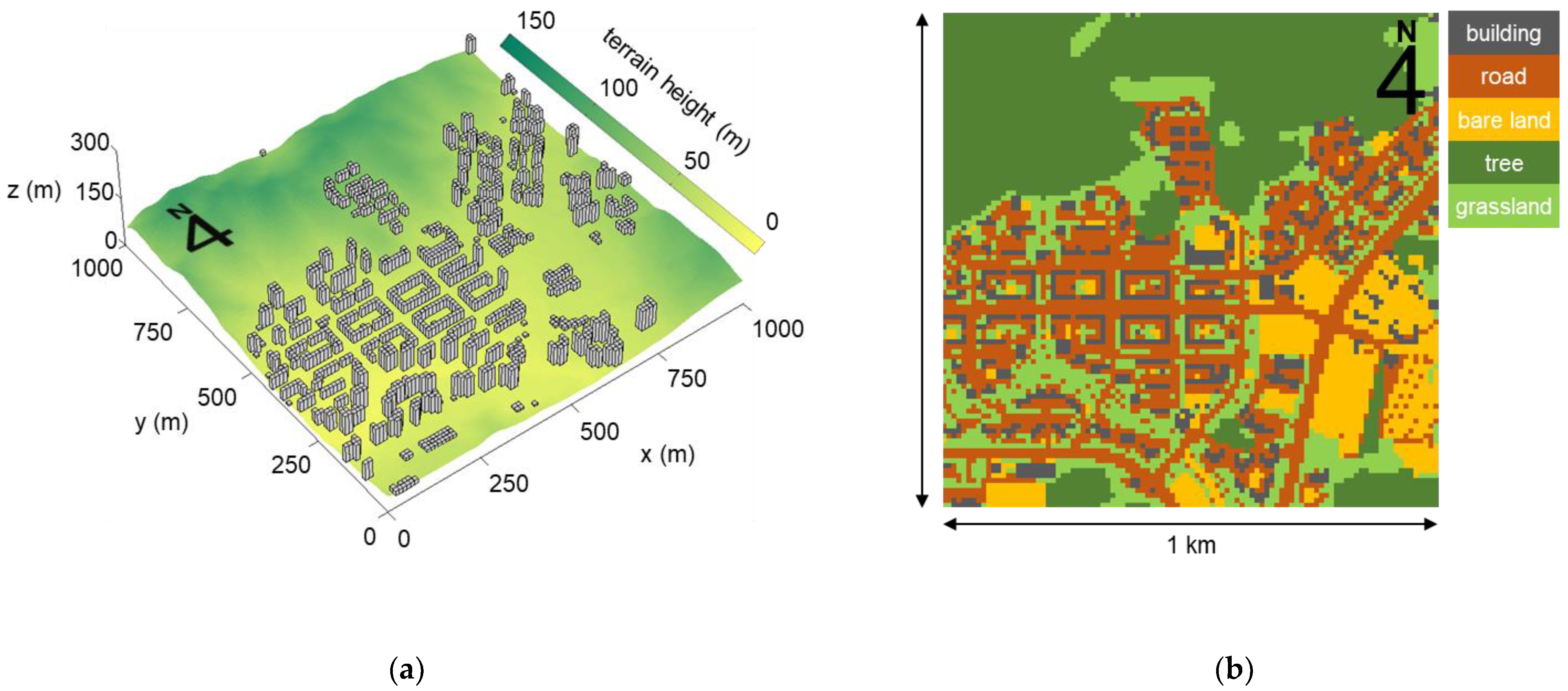
2.4. Numerical Setup

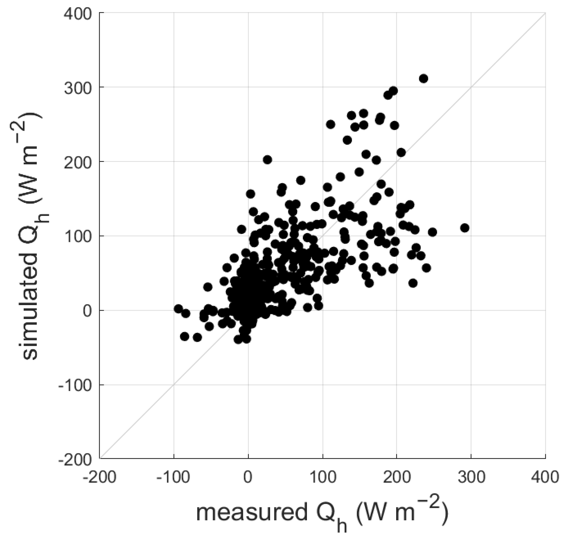
The numerical domain was set according to Cost Action 732, a guideline for the numerical simulation of the CFD model. COST Action 732 states that when calculating for an urban area, the top boundary of the numerical domain should be at least 5 times the height of the tallest building (H_max) away from the height of the building. However, the lateral boundaries are not required to be 5 H_max away from the tallest building. COST action 732 provides a standard that considers only the building and does not provide a standard that considers both the topography and the building. In this study, the highest altitude considered includes both topography and building heights as H_max. Therefore, the model domain sizes considered in this study were 2000 m, 2000 m, and 630 m in the x, y, and z directions, respectively (horizontally 4.8 H_max, vertically 5.1 H_max). The target area is 1000 m by 1000 m. The grid numbers (sizes) are 200 (10 m), 200 (10 m), and 315 (2 m) in the x, y, and z directions, respectively. The topography and building boundaries in the CFD model were constructed using a Geographic Information System (GIS) established by the National Geographic Information Institute of Korea in 2015 (Figure 2). The GIS provides topography contours in a vector format and building information in a raster format with a 1 m resolution. Since the horizontal grid size of the CFD model is 10 m by 10 m, we classified a grid as a building if it contained more than 55% GIS buildings within it and as non-building if it contained less than 55%. The target area considered the actual topography and buildings, and the boundary area considered only the actual topography (in Figure 3a).

In this study, the CFD model was combined with the Local Data Assimilation and Prediction System (LDAPS) and the Vegetation Urban Canopy Model (VUCM) developed by Lee and Park [28] (hereafter, noted as LCV) to simulate Q_h more accurately in urban areas. The LDAPS, one of the numerical weather forecasting systems operated by the Korea Meteorological Administration (KMA), provided the boundary and initial conditions for the CFD model simulations every hour during the target period. The LDAPS is based on the unified model [41,42] of the Met Office, UK, and uses an Arakawa C-grid [43] for the horizontal–vertical grid system and a Charney–Phillips grid staggering [44] for the vertical grid system. The LDAPS has a horizontal resolution of 1.5 km and consists of 744 grids in the east–west direction and 928 grids in the north–south direction. It has a vertical extent of up to 39 km with 70 layers. The time integration method of the LDAPS is semi-implicit and semi-Lagrangian. The LDAPS conducts 36 h predictions for weather forecasting at 00, 06, 12, and 18 UTC and 3 h predictions for providing background fields to the 36 h predictions at 03, 09, 15, and 21 UTC. The 3 h forecasting data (horizontal wind components and air temperatures) of the LDAPS provided the boundary and initial conditions for the CFD model. The wind and temperature data of the LDAPS were used by vertically interpolating them according to the vertical grid system of the CFD model. Wind and temperature data at the four closest LDAPS grid points around the target area were averaged and used as the initial conditions for the CFD model.

For the prescription of the land surface temperatures, the sub-divided land cover map, and the VUCM were used. The sub-divided land cover map, provided by the Environmental Geographic Information Service (EGIS) of the Ministry of Environment of Korea, divides the land into 41 different cover classes with a 1 m resolution. It was reclassified into building, road, bare land, grassland, and tree areas (Figure 3b). The land surface temperatures of the five sub-divided land cover types (building, road, bare land, grassland, and tree) were simulated using the VUCM, developed by Lee and Park [28]. The VUCM parameterizes the physical processes within urban canopy layers, such as long- and short-wave radiation transfer, heat transfer between artificial surfaces (roof, road, and soil), and the hydrological process by urban vegetation. It can diagnose the air temperature, humidity, wind speeds, and land surface temperatures (roof, wall, and bottom) of street canyons, with input variables that reflect meteorological forcing and urban morphology. VUCM simulation results for the target area’s land surface temperature were used, and the LDAPS temperature was used for the boundary area’s land surface temperature.

3. Model Validation

Before validating the simulated Q_h, the performance of the CFD model was validated for the period of 15 September 2014 to 21 September 2014 against the wind speeds, wind directions, and temperatures measured at the flux tower (Figure 4). The temperatures simulated by both the CFD model and the LDAPS were similar to the measurements. The root mean square error (RMSE) of the temperature was 1.19 °C for the LDAPS and 1.24 °C for the CFD model. The LDAPS overestimated the measured wind speeds, and the CFD model slightly improved the reproduction of the measured wind speeds (LDAPS RMSE = 1.69 m s⁻¹, CFD RMSE = 1.19 m s⁻¹). The wind speed overestimation of the LDAPS resulted from the coarser horizontal resolution (1.5 km), which is not small enough to resolve the subgrid-scale obstacles and buildings. The RMSEs for wind directions were similar for both the LDAPS and the CFD model (LDAPS = 87.53°, CFD = 90.26°). The measurements at the flux tower showed that the northeasterly (28.57%), northerly (16.07%), and northwesterly (7.14%) winds were dominant. The CFD (LDAPS) model simulated the wind directions measured at the flux tower relatively well, with 50.00% (41.67%) of the northeasterlies, 16.67% (20.83%) of the northerlies, and 4.17% (8.33%) of the easterlies.

4. Results and Discussions

Q_h was calculated as follows [12]:

$$Q_h=\rho ·C_p·\overline{w^{’}{T}^{’}}$$

(12)

Here, $\rho$ and $C_p$ are the dry air density (=1.2 ${\mathrm{k}\mathrm{g}\mathrm{m}}^{-3}$) and specific heat at constant pressure (=1012 ${\mathrm{J}\mathrm{k}\mathrm{g}}^{-1}{\mathrm{K}}^{-1}$), respectively, and $w^{’}$ and $T^{’}$ denote the perturbations from the mean vertical wind component ($w$) and temperature ($T$), respectively. In the CFD model, the turbulent heat flux ($-\overline{w^{’}{T}^{’}}$) is parameterized in terms of the turbulent heat diffusivity ($K_h$) and vertical temperature gradient ($\partial T/\partial z$) as ($-\overline{w^{’}{T}^{’}}=K_h\partial T/\partial z$). The turbulent heat diffusivity ($K_h$) is defined as the ratio of turbulent momentum diffusivity ($K_m$) to turbulent Prandtl number (${Pr}_t$, 0.9) as $K_h=\frac{K_m}{{Pr}_t}$.

Q_h was calculated once every hour from 1 September 2014 to 30 September 2014. Figure 5 is a scatter plot of Q_h values measured by the flux tower and simulated by the LCV during the target period. The simulated Q_h was also evaluated using statistical indices such as the root mean square error (RMSE), mean absolute error (MAE), index of agreement (IOA), and correlation coefficient (R), defined as follows:

$$RMSE=\sqrt{\frac{1}{N}\sum {\left(S-M\right)}^2}$$

(13)

$$MAE=\frac{1}{N}\sum \left|\left(S-M\right)\right|$$

(14)

$$IOA=1-\frac{\sum {\left(S-M\right)}^2}{\sum {\left(\left|S-\overline{M}\right|+\left|M-\overline{M}\right|\right)}^2}$$

(15)

$$R=\frac{\sum \left(S-\overline{S}\right)\left(M-\overline{M}\right)}{\sqrt{\sum {\left(S-\overline{S}\right)}^2\sum {\left(M-\overline{M}\right)}^2}}$$

(16)

where S and M indicate the simulated and measured Q_h, respectively. $\overline{S}$ and $\overline{M}$ indicate the averages of S and M, respectively. MAE and IOA range from 0 to 1, where MAE being 0 and IOA being 1 signify perfect agreement between the model and measurements [45,46,47]. RMSE, MAE, IOA, and R for the target period are 42.68 ${\mathrm{W}\mathrm{m}}^{-2}$, 26.95 ${\mathrm{W}\mathrm{m}}^{-2}$, 0.84, and 0.73, respectively (

Table 1. Statistical values of numerically simulated sensible heat flux at the flux tower from 1 September 2014 to 30 September 2014.

	RMSE [W m−2]	$\mathbf{MAE}[{\mathbf{W}\mathbf{m}}^{-2}$]	IOA	R
all day	42.68	26.95	0.84	0.73
day	58.61	42.35	0.77	0.60
night	21.22	13.78	0.41	0.15
sunny day	47.00	29.81	0.85	0.73
cloudy day	35.76	23.05	0.81	0.68

).

This study compared the accuracy (performance) of simulated Q_h values with prior research findings [14,15,48]. Rios and Ramamurthy [48] utilized a numerical model that used land surface temperature data acquired from satellites from June 2019 to May 2020 to estimate Q_h. They validated the model using Q_h measurements obtained from three flux tower locations in New York City. The RMSEs for the numerically simulated Q_h values at the three locations were 59.26 ${\mathrm{W}\mathrm{m}}^{-2}$, 43.52 ${\mathrm{W}\mathrm{m}}^{-2}$, 36.21 ${\mathrm{W}\mathrm{m}}^{-2}$, respectively. Feigenwinter et al. [14] estimated Q_h values for the Swiss Basel region with a spatial resolution of 100 m, using data collected from satellites during a period of 22 measurements from February 2013 to December 2015. They verified their estimates using the measured Q_h values from three flux towers. The RMSEs at the three locations were 66 W m⁻², 57 W m⁻², and 34 W m⁻², respectively. Machado et al. [15] simulated Q_h for Cuiabá, Brazil, from April to November 2009 using satellite data and a numerical model. When they validated the simulated Q_h against the measured data, the RMSE, MAE, IOA, and R values were 32.6 W m⁻², 26.8 W m⁻², 0.84, and 0.76, respectively. The performance of the numerical Q_h modeling in this study compares favorably with previous research, and it is considered suitable for analyzing the spatial distribution of Q_h in urban areas. The studies by Feigenwinter et al. [14], Rios and Ramamurthy [48], and Machado et al. [15] estimated Q_h based on satellite measurement data. However, these studies faced challenges in continuous Q_h estimation due to varying meteorological conditions and measurement timing.

Figure 6 shows the diurnal variation in the time-averaged Q_h, both measured and numerically simulated, at the flux tower. The measured Q_h ranged from −6.92 W m⁻² to 2.07 W m⁻² during the nighttime. The highest Q_h occurred at 13 LST, reaching 153.52 W m⁻². The LCV closely simulated the diurnal trends in the measured Q_h. However, the LCV results did not exhibit a downward trend in Q_h values during the nighttime. In particular, at 19 LST, just after sunset, the model overestimated Q_h compared to the measurements (model: 24.82 W m⁻², measured: 2.07 W m⁻²). The LCV simulated the highest Q_h (122.04 W m⁻²) at 13 LST. It underestimated Q_h from 10 to 14 LST and overestimated it from 17 to 20 LST.

LCV’s simulated Q_h closely resembled prior research findings [49,50]. LCV similarly simulated the temperature measured at the flux tower. A comparison was conducted between the land surface temperature measured during the target period at the Seoul Automated Synoptic Observing System (37.5714° N, 126.9658° E), located approximately 7.8 km southwest of the flux tower, and the land surface temperature used in this study. The observatory has a grassy surface, while the temperature measurement point is on bare land. Since the land cover type differs between the measurement point and the flux tower location, the time-averaged temperatures were compared after normalization through Z-Score Standardization (Figure 7). The VUCM underestimated the surface temperature during 07–14 LST and overestimated it during 16–20 LST. In other words, the modeling performance of Q_h was sensitive to the surface temperature, with Q_h being underestimated (overestimated) during times when the surface temperature was underestimated (overestimated). Although there were some discrepancies between the meteorological elements simulated by the LCV and the measurements, the statistical analysis of the simulated Q_h in this study showed reliable values when compared with previous studies. Moreover, the diurnal variations displayed patterns that were not only similar to the measurements but also aligned closely with previous findings, suggesting that analyzing the spatial distribution in this study is appropriate.

Figure 8 illustrates the averaged distribution of Q_h over the entire period. A distinct contrast is evident in the Q_h distribution by land cover types, with higher values in areas with buildings, roads, and bare land, and lower values in vegetated areas such as trees and grasslands. The average Q_h values for building, road, bare land, grassland, and tree areas were 36.79, 11.96, 27.77, 1.94, and −3.04 W m⁻², respectively. Notably, a downward Q_h is observed in the extensive tree and grassland areas (Figure 8e,f). Feigenwinter et al. [14] reported that at around 11 a.m., Q_h was the highest in impermeable land cover areas (urban areas) and either approached 0 W m⁻² or had a downward Q_h value in tree (dense forest) areas. Tan et al. [8] analyzed the impact of trees in densely populated areas of Hong Kong on Q_h and also observed a downward Q_h trend during summer at noontime in tree areas. In areas located between buildings, the turbulent heat diffusivity was smaller, and the vertical temperature gradient decreased due to the influence of building shadows. As a result, the average Q_h in road areas was lower than that in bare land areas. Figure 9 represents the spatial distribution of the standard deviation of the time-averaged Q_h values during the target period. The standard deviation was higher in areas with higher sensible heat fluxes. Specifically, the standard deviation was highest in building areas with an average of 51.28 W m⁻² and lowest in grassland areas with an average of 16.35 W m⁻².

Figure 10 displays the hourly variation in the time-averaged Q_h values throughout the entire target period. Q_h exhibited distinct diurnal trends depending on the land cover type. The average Q_h in building, road, and bare land areas was highest at 14 LST (103.30 W m⁻², 30.77 W m⁻², and 57.41 W m⁻², respectively). However, the minimum average Q_h in building areas occurred at 5 LST (1.14 W m⁻²), while in road and bare land areas, it occurred at 4 LST (2.93 W m⁻² and 11.28 W m⁻²). In areas with trees and grassland, the average Q_h mainly exhibited a downward trend during the afternoon. Upward Q_h was highest at 9 LST (21.64 W m⁻²) for trees and 12 LST (11.86 W m⁻²) for grassland, while the downward Q_h peaked at 17 LST (trees: −29.37 W m⁻², grassland: −5.95 W m⁻²). Furthermore, at 22 LST (1.07 W m⁻²) for trees and 23 LST (−0.64 W m⁻²) for grassland, the average Q_h was the lowest. Notably, while the average Q_h in building, road, and bare land areas was highest at 14 LST, it was significantly lower in areas with trees and grassland (−19.75 W m⁻² and 5.84 W m⁻², respectively). The spatial distribution of the simulated hourly Q_h values in this study closely resembles the results obtained by Rios and Ramamurthy [48]. It simulated Q_h below 100 W m⁻² around 10 LST and Q_h near 0 W m⁻² after sunset. Additionally, Q_h was highest in most areas at 13 LST, but lower in areas with vegetation compared to other regions.

In this study, the factors determining the magnitude of Q_h are the vertical temperature gradient and turbulent heat diffusivity. In the case of road, building, and barren land areas, both the average vertical temperature gradient and turbulent heat diffusivity were higher during the daytime compared to the nighttime, except for the period just after sunrise (Figure 11). Similarly, grasslands and tree-covered areas also showed higher average turbulent heat diffusivities during the daytime, but the average vertical temperature gradient in these areas was exceptionally low during certain daytime hours, coinciding with times when the average Q_h was simulated to be low. In the case of building, barren land, and grassland areas, even when the average turbulent heat diffusivity was not relatively high during the time when Q_h was highest, the contribution of the average vertical temperature gradient was significant. On the other hand, both the average turbulent heat diffusivity and average vertical temperature gradient were relatively high in road and tree areas.

Within the target area, during the nighttime (19 to 06 LST), Q_h did not exhibit significant spatial variability and showed relatively small differences among land cover types. However, during the daytime (07 to 18 LST), even for the same land cover type, there were substantial spatial variations (Figure 11c). This was attributed to larger differences in the distribution of the vertical temperature gradients and turbulent heat diffusivity during the daytime compared to nighttime. For example, the interquartile range (Q3–Q1) of the vertical temperature gradient in the building area was about 6.23 times larger at 14 LST (maximum) than at 05 LST (minimum), which was the greatest among all land cover types. Similarly, the interquartile range of turbulent heat diffusivity in the road area was approximately 3.83 times larger at 09 LST (maximum) than at 04 LST (minimum).

During the daytime, the Q_h calculated on the rooftop of building areas was the highest, but they were lower compared to road, barren land, and tree areas during the nighttime. In terms of the mean values, Q_h showed relatively constant values in the range of 1.13 (at 05 LST) to 4.04 W m⁻² (at 01 LST) from 00 to 07 LST but increased from 08 LST, reaching its maximum at 14 LST, followed by a decrease. The diurnal trend of the mean Q_h in the road area was similar to that in the building area, exhibiting constant values in the morning, an increase from 08 to 14 LST, and a subsequent decrease. However, in most areas around the buildings in the road area, due to the low turbulent heat diffusivity and the influence of building shadows, many Q_h values were low (below median 14.76 W m⁻²). The mean Q_h in the bare land area was highest during the nighttime (except for 19 LST) and second highest during the daytime, following the building area. The high Q_h in the bare land area was found to be a result of the fact that, in the target area, bare areas were mostly located at some distance from the buildings. However, similar to the road area located near buildings, a low Q_h was observed in the bare areas near buildings (Figure 8d). The grassland area exhibited the smallest temporal variation (17.82 W m⁻²) in the mean Q_h, and the interquartile range of the mean was the smallest (10.71 W m⁻²). The median mean Qh was 0.78 W m⁻², and the upward Q_h (around buildings and roads) and downward Q_h (near the tree area) were distributed at similar magnitudes at all times. In the tree area, the mean Q_h reached its maximum upward Q_h at 09 LST, followed by a downward Q_h from 12 LST, reaching its maximum downward Q_h at 17 LST. Furthermore, from 13 to 23 LST, a downward Q_h was simulated in most areas (below Q2). In open bare areas without nearby buildings, Q_h exhibited patterns similar to those in building areas, indicating significant variations in Q_h values due to the surrounding environment, even for the same land cover type.

5. Conclusions

This study developed an LCV based on a CFD model that is capable of conducting high-resolution simulations to simulate the sensible heat flux in urban areas with various land cover types. Simulations were conducted at a horizontal grid resolution of 10 m over a 1 km² area for one month (September 2014) with hourly intervals, and the spatial distribution of the sensible heat flux was analyzed. To obtain realistic sensible heat flux estimates, wind and temperature data from LDAPS, along with land surface temperatures categorized by land cover type from VUCM, were utilized. The land cover was classified into five categories (buildings, roads, bare land, grassland, and tree areas). Before analyzing the spatial distribution of the sensible heat flux, the LCV’s performance was validated using wind speed, wind direction, temperature, and sensible heat flux measurements obtained from flux towers within the target area.

Throughout the entire target period, buildings, roads, and bare land areas generally exhibited upward sensible heat fluxes in most regions, while grassland and tree areas featured downward sensible heat fluxes over extensive areas. Conversely, areas such as roads, bare land, and grassland situated between buildings showed relatively lower sensible heat fluxes compared to regions farther away from buildings due to lower vertical temperature gradients and a turbulent heat diffusivity. The diurnal variation in the sensible heat flux’s spatial distribution revealed a daytime dominance of higher values, followed by lower values during nighttime for buildings, roads, and bare land areas. Tree areas exhibited a maximum upward sensible heat flux in the morning, followed by a maximum downward flux in the afternoon. Grassland areas displayed less significant temporal variability compared to other land cover types.

The urban sensible heat flux distribution showed distinct characteristics based on land cover types. Notably, the sensible heat flux from building rooftops was particularly high, signifying its substantial influence on the urban thermal environment. Although the analysis focused on the sensible heat fluxes of building rooftops, it is important to acknowledge that building wall surface temperature variations could lead to different characteristics in the wall-level sensible heat flux. Reducing the sensible heat flux from buildings could potentially contribute to improvements in the urban thermal environment.

In the future, it is considered necessary to conduct additional research through high-resolution numerical simulations to explore ways to reduce the sensible heat flux from urban buildings and assess their impact on strategies for mitigating the urban thermal environment. Additionally, the study revealed that bare land areas also exhibited high sensible heat flux values. Based on these findings, it is suggested that reducing the proportion of bare land or converting it to grassland or tree areas may be necessary for enhancing the urban thermal environment.

The method for estimating the spatial distribution of a sensible heat flux using the CFD model, as presented in this study, is considered effective in simulating sensible heat flux according to the land cover types that are typically found in urban areas. The proposed approach is anticipated to provide valuable insights into strategies for improving the thermal environment in urban areas that require heat mitigation. Analyzing areas with varying thermal conditions, identifying regions that are vulnerable to heatwaves and cold spells, and developing corresponding mitigation strategies are among the potential applications. Furthermore, the analysis of the sensible heat flux in urban areas based on various land cover ratios can be used to develop thermal environment scenarios and contribute to urban planning efforts aimed at enhancing the urban environment.

References

1. Nadeau, D.F.; Brutsaert, W.; Parlange, M.B.; Bou-Zeid, E.; Barrenetxea, G.; Couach, O.; Boldi, M.-O.; Selker, J.S.; Vetterli, M. Estimation of urban sensible heat flux using a dense wireless network of observations. Environ. Fluid Mech. 2009, 9, 635–653. [Google Scholar] [CrossRef]
2. Hong, J.W.; Hong, J. Changes in the Seoul metropolitan area urban heat environment with residential redevelopment. J. Appl. Meteorol. Climatol. 2016, 55, 1091–1106. [Google Scholar] [CrossRef]
3. Marelle, L.; Myhre, G.; Steensen, B.M.; Hodnebrog, Ø.; Alterskjær, K.; Sillmann, J. Urbanization in megacities increases the frequency of extreme precipitation events far more than their intensity. Environ. Res. Lett. 2020, 15, 124072. [Google Scholar] [CrossRef]
4. Pham, J.V.; Baniassadi, A.; Brown, K.E.; Heusinger, J.; Sailor, D.J. Comparing photovoltaic and reflective shade surfaces in the urban environment: Effects on surface sensible heat flux and pedestrian thermal comfort. Urban Clim. 2019, 29, 100500. [Google Scholar] [CrossRef]
5. Scherba, A.; Sailor, D.J.; Rosenstiel, T.N.; Wamser, C.C. Modeling impacts of roof reflectivity, integrated photovoltaic panels and green roof systems on sensible heat flux into the urban environment. Build. Environ. 2011, 46, 2542–2551. [Google Scholar] [CrossRef]
6. Coutts, A.M.; Daly, E.; Beringer, J.; Tapper, N.J. Assessing practical measures to reduce urban heat: Green and cool roofs. Build. Environ. 2013, 70, 266–276. [Google Scholar] [CrossRef]
7. Song, H.J.; Lim, B.; Joo, S. Evaluation of rainfall forecasts with heavy rain types in the high-resolution unified model over South Korea. Weather Forecast. 2019, 34, 1277–1293. [Google Scholar] [CrossRef]
8. Tan, Z.; Lau, K.K.L.; Ng, E. Urban tree design approaches for mitigating daytime urban heat island effects in a high-density urban environment. Energy Build. 2016, 114, 265–274. [Google Scholar] [CrossRef]
9. Xu, X.; Asawa, T. Systematic numerical study on the effect of thermal properties of building surface on its temperature and sensible heat flux. Build. Environ. 2020, 168, 106485. [Google Scholar] [CrossRef]
10. Takahashi, K.; Yoshida, H.; Tanaka, Y.; Aotake, N.; Wang, F. Measurement of thermal environment in Kyoto city and its prediction by CFD simulation. Energy Build. 2004, 36, 771–779. [Google Scholar] [CrossRef]
11. Xu, W.; Wooster, M.J.; Grimmond, C.S.B. Modelling of urban sensible heat flux at multiple spatial scales: A demonstration using airborne hyperspectral imagery of Shanghai and a temperature–emissivity separation approach. Remote Sens. Environ. 2008, 112, 3493–3510. [Google Scholar] [CrossRef]
12. Salamanca, F.; Martilli, A. A new building energy model coupled with an urban canopy parameterization for urban climate simulations—Part II. Validation with one dimension off-line simulations. Theor. Appl. Climatol. 2010, 99, 345–356. [Google Scholar] [CrossRef]
13. Barlow, J.F.; Halios, C.H.; Lane, S.E.; Wood, C.R. Observations of urban boundary layer structure during a strong urban heat island event. Environ. Fluid Mech. 2015, 15, 373–398. [Google Scholar] [CrossRef]
14. Feigenwinter, C.; Vogt, R.; Parlow, E.; Lindberg, F.; Marconcini, M.; Del Frate, F.; Chrysoulakis, N. Spatial distribution of sensible and latent heat flux in the city of Basel (Switzerland). IEEE J. Sel. Top. Appl. Earth Obs. Remote Sens. 2018, 11, 2717–2723. [Google Scholar] [CrossRef]
15. Machado, N.G.; Biudes, M.S.; Angelini, L.P.; Querino, C.A.S.; da Silva Angelini, P.C.B. Impact of Changes in surface cover on energy balance in a tropical city by remote sensing: A study case in Brazil. Remote Sens. Appl. 2020, 20, 100373. [Google Scholar] [CrossRef]
16. Kato, S.; Yamaguchi, Y. Analysis of urban heat-island effect using ASTER and ETM+ Data: Separation of anthropogenic heat discharge and natural heat radiation from sensible heat flux. Remote Sens. Environ. 2005, 99, 44–54. [Google Scholar] [CrossRef]
17. Zhang, N.; Wang, X.; Peng, Z. Large-eddy simulation of mesoscale circulations forced by inhomogeneous urban heat island. Bound.-Layer Meteor. 2014, 151, 179–194. [Google Scholar] [CrossRef]
18. Antoniou, N.; Montazeri, H.; Neophytou, M.; Blocken, B. CFD simulation of urban microclimate: Validation using high-resolution field measurements. Sci. Total Environ. 2019, 695, 133743. [Google Scholar] [CrossRef] [PubMed]
19. Zhang, S.; Kwok, K.C.; Liu, H.; Jiang, Y.; Dong, K.; Wang, B. A CFD study of wind assessment in urban topology with complex wind flow. Sustain. Cities Soc. 2021, 71, 103006. [Google Scholar] [CrossRef]
20. Brozovsky, J.; Simonsen, A.; Gaitani, N. Validation of a CFD model for the evaluation of urban microclimate at high latitudes: A case study in Trondheim, Norway. Build. Environ. 2021, 205, 108175. [Google Scholar] [CrossRef]
21. Brozovsky, J.; Radivojevic, J.; Simonsen, A. Assessing the impact of urban microclimate on building energy demand by coupling CFD and building performance simulation. J. Build. Eng. 2022, 55, 104681. [Google Scholar] [CrossRef]
22. Moradpour, M.; Hosseini, V. An investigation into the effects of green space on air quality of an urban area using CFD modeling. Urban Clim. 2020, 34, 100686. [Google Scholar] [CrossRef]
23. Lee, S.; Park, S.Y.; Kim, J.J.; Kim, M.J. Thermal effects on dispersion of secondary inorganic aerosols in an urban street canyon. Urban Clim. 2023, 47, 101375. [Google Scholar] [CrossRef]
24. Maggiotto, G.; Buccolieri, R.; Santo, M.A.; Leo, L.S.; Di Sabatino, S. Validation of temperature-perturbation and CFD-based modelling for the prediction of the thermal urban environment: The Lecce (IT) case study. Environ. Model. Softw. 2014, 60, 69–83. [Google Scholar] [CrossRef]
25. Huang, H.; Ooka, R.; Kato, S. Urban thermal environment measurements and numerical simulation for an actual complex urban area covering a large district heating and cooling system in summer. Atmos. Environ. 2005, 39, 6362–6375. [Google Scholar] [CrossRef]
26. Ashie, Y.; Kono, T. Urban-scale CFD analysis in support of a climate-sensitive design for the Tokyo Bay area. Int. J. Climatol. 2011, 31, 174–188. [Google Scholar] [CrossRef]
27. Allegrini, J.; Dorer, V.; Carmeliet, J. Coupled CFD, radiation and building energy model for studying heat fluxes in an urban environment with generic building configurations. Sustain. Cities Soc. 2015, 19, 385–394. [Google Scholar] [CrossRef]
28. Lee, S.H.; Park, S.U. A vegetated urban canopy model for meteorological and environmental modelling. Bound.-Layer Meteor. 2008, 126, 73–102. [Google Scholar] [CrossRef]
29. Patankar, S. Numerical Heat Transfer and Fluid Flow; CRC Press: Boca Raton, FL, USA, 2018. [Google Scholar]
30. Yakhot, V.; Orszag, S.A.; Thangam, S.; Gatski, T.B.; Speziale, C. Development of turbulence models for shear flows by a double expansion technique. Phys. Fluids A. 1992, 4, 1510–1520. [Google Scholar] [CrossRef]
31. Versteeg, H.K.; Malalasekera, W. An Introduction to Computational Fluid Dynamics: The Finite Volume Method; Longman: London, England, 1995; p. 257. [Google Scholar]
32. Kim, J.J.; Baik, J.J. Effects of street-bottom and building-roof heating on flow in three-dimensional street canyons. Adv. Atmos. Sci. 2010, 27, 513–527. [Google Scholar] [CrossRef]
33. Park, S.J.; Kim, J.J.; Kim, M.J.; Park, R.J.; Cheong, H.B. Characteristics of flow and reactive pollutant dispersion in urban street canyons. Atmos. Environ. 2015, 108, 20–31. [Google Scholar] [CrossRef]
34. Park, S.J.; Choi, W.; Kim, J.J.; Kim, M.J.; Park, R.J.; Han, K.S.; Kang, G. Effects of building–roof cooling on the flow and dispersion of reactive pollutants in an idealized urban street canyon. Build. Environ. 2016, 109, 175–189. [Google Scholar] [CrossRef]
35. Kang, G.; Kim, J.J.; Kim, D.J.; Choi, W.; Park, S.J. Development of a computational fluid dynamics model with tree drag parameterizations: Application to pedestrian wind comfort in an urban area. Build. Environ. 2017, 124, 209–218. [Google Scholar] [CrossRef]
36. Kang, G.; Kim, J.J. Effects of Vertical Forests on Air Quality in Step-up Street Canyons. Sustain. Cities Soc. 2023, 94, 104537. [Google Scholar] [CrossRef]
37. Hayati, A.N.; Stoll, R.; Kim, J.J.; Harman, T.; Nelson, M.A.; Brown, M.J.; Pardyjak, E.R. Comprehensive evaluation of fast-response, Reynolds-averaged Navier–Stokes, and large-eddy simulation methods against high-spatial-resolution wind-tunnel data in step-down street canyons. Bound.-Layer Meteor. 2017, 164, 217–247. [Google Scholar] [CrossRef]
38. Hayati, A.N.; Stoll, R.; Pardyjak, E.R.; Harman, T.; Kim, J.J. Comparative metrics for computational approaches in non-uniform street-canyon flows. Build. Environ. 2019, 158, 16–27. [Google Scholar] [CrossRef]
39. Baik, J.J.; Park, S.B.; Kim, J.J. Urban flow and dispersion simulation using a CFD model coupled to a mesoscale model. J. Appl. Meteorol. Climatol. 2009, 48, 1667–1681. [Google Scholar] [CrossRef]
40. Kang, G.; Kim, J.J.; Choi, W. Computational fluid dynamics simulation of tree effects on pedestrian wind comfort in an urban area. Sustain. Cities Soc. 2020, 56, 102086. [Google Scholar] [CrossRef]
41. Park, I.; Kim, H.S.; Lee, J.; Kim, J.H.; Song, C.H.; Kim, H.K. Temperature prediction using the missing data refinement model based on a long short-term memory neural network. Atmosphere 2019, 10, 718. [Google Scholar] [CrossRef]
42. Song, J.; Wang, Z.H.; Wang, C. The regional impact of urban heat mitigation strategies on planetary boundary layer dynamics over a semiarid city. J. Geophys. Res. Atmos. 2018, 123, 6410–6422. [Google Scholar] [CrossRef]
43. Arakawa, A.; Lamb, V.R. Computational design of the basic dynamical process of the UCLA general circulation model. Methods Comput. Phys. 1977, 17, 173–265. [Google Scholar]
44. Charney, J.G.; Philips, N.A. Numerical integration of the quasi-geostrophic equations for barotropic and simple baroclinic flow. J. Meteorol. 1953, 10, 71–99. [Google Scholar] [CrossRef]
45. Bürger, C.M.; Kolditz, O.; Fowler, H.J.; Blenkinsop, S. Future climate scenarios and rainfall–runoff modelling in the Upper Gallego catchment (Spain). Environ. Pollut. 2007, 148, 842–854. [Google Scholar] [CrossRef] [PubMed]
46. Feng, Y.; Jia, Y.; Zhang, Q.; Gong, D.; Cui, N. National-scale assessment of pan evaporation models across different climatic zones of China. J. Hydrol. 2018, 564, 314–328. [Google Scholar] [CrossRef]
47. Wang, Y.; Chan, A.; Lau, G.N.C.; Li, Q.; Yang, Y.; Yim, S.H.L. Effects of urbanization and global climate change on regional climate in the Pearl River Delta and thermal comfort implications. Int. J. Climatol. 2019, 39, 2984–2997. [Google Scholar] [CrossRef]
48. Rios, G.; Ramamurthy, P. A novel model to estimate sensible heat fluxes in urban areas using satellite-derived data. Remote Sens. Environ. 2022, 270, 112880. [Google Scholar] [CrossRef]
49. Lian-Tong, Z.; Ren-Guang, W.; Rong-Hui, H. Variability of surface sensible heat flux over Northwest China. Atmos. Ocean. Sci. Lett. 2010, 3, 75–80. [Google Scholar] [CrossRef]
50. Zieliński, M.; Fortuniak, K.; Pawlak, W.; Siedlecki, M. Long-term turbulent sensible-heat-flux measurements with a large-aperture scintillometer in the Centre of Łódź, Central Poland. Bound.-Layer Meteor. 2018, 167, 469–492. [Google Scholar] [CrossRef]
Figure 1. A satellite image of the target area (image source: https://map.naver.com, accessed on 25 April 2024). The red dots indicate the locations of the flux towers where sensible heat flux (Qh) measurements were conducted.
Atmosphere 15 00681 g001
Figure 2. Schematic representation of input data for the CFD model used in sensible heat flux simulations.
Atmosphere 15 00681 g002
Figure 3. (a) Three-dimensional building and topography input data for the target area and (b) land cover distribution in the target area.
Atmosphere 15 00681 g003
Figure 4. Time series of temperature, wind speed, and wind direction measured and numerically simulated at the flux tower from 15 September 2014 to 21 September 2014.
Atmosphere 15 00681 g004
Figure 5. Comparison of numerically simulated sensible heat flux and measurements taken at the flux tower from 1 September 2014 to 30 September 2014.
Atmosphere 15 00681 g005
Figure 6. Diurnal variation in time-averaged sensible heat flux and its standard deviation at each hour, measured at the flux tower from 1 September 2014 to 30 September 2014.
Atmosphere 15 00681 g006
Figure 7. Diurnal variation in time-averaged normalized land surface temperature, measured at the flux tower from 1 September 2014 to 30 September 2014.
Atmosphere 15 00681 g007
Figure 8. Distribution of numerically simulated sensible heat fluxes in September 2014 by LCV for (a) the entire area, (b) building areas, (c) road areas, (d) bare land areas, (e) grassland areas, and (f) tree areas.
Atmosphere 15 00681 g008
Figure 9. Distribution of standard deviation of numerically simulated sensible heat fluxes in September 2014 by LCV for (a) the entire area, (b) building areas, (c) road areas, (d) bare land areas, (e) grassland areas, and (f) tree areas.
Atmosphere 15 00681 g009
Figure 10. Time-averaged sensible heat flux distribution in September 2014 by LST (Local Solar Time) for (a) 04 LST, (b) 09 LST, (c) 12 LST, (d) 14 LST, (e) 17 LST, and (f) 22 LST.
Atmosphere 15 00681 g010
Figure 11. Box plots of (a) temperature gradients, (b) turbulent heat diffusivity, and (c) sensible heat flux by land cover type, time-averaged in September 2014.
Atmosphere 15 00681 g011