Abstract
The Upper Hunter Valley is a major coal mining area in New South Wales (NSW), Australia. Due to the ongoing increase in mining activities, PM10 (air-borne particles with an aerodynamic diameter less than 10 micrometres) pollution has become a major air quality concern in local communities. The present study was initiated to quantitatively examine the spatial and temporal variability of PM10 pollution in the region. An earlier paper of this study identified two air quality subregions in the valley. This paper aims to provide a holistic summarisation of the relationships between elevated PM10 pollution in two subregions and the local- and synoptic-scale meteorological conditions for spring and summer, when PM10 pollution is relatively high. A catalogue of twelve synoptic types and a set of six local meteorological patterns were quantitatively derived and linked to each other using the self-organising map (SOM) technique. The complex meteorology–air pollution relationships were visualised and interpreted on the SOM planes for two representative locations. It was found that the influence of local meteorological patterns differed significantly for mean PM10 levels vs. the occurrence of elevated pollution events and between air quality subregions. In contrast, synoptic types showed generally similar relationships with mean vs. elevated PM10 pollution in the valley. Two local meteorological patterns, the hot–dry–northwesterly wind conditions and the hot–dry–calm conditions, were found to be the most PM10 pollution conducive in the valley when combined with a set of synoptic counterparts. These synoptic types are featured with the influence of an eastward migrating continental high-pressure system and westerly troughs, or a ridge extending northwest towards coastal northern NSW or southern Queensland from the Tasman Sea. The method and results can be used in air quality research for other locations of NSW, or similar regions elsewhere.
1. Introduction
The Upper Hunter Valley is a major coal mining area located within the northwestern end of the Hunter region, around 200 km north of Sydney and 50 km northwest of Newcastle in the State of New South Wales (NSW), Australia (Figure 1) [1,2]. PM10 (air-borne particles with an aerodynamic diameter less than 10 micrometres) pollution has become a major air quality concern in local communities, primarily due to the ongoing increase in open-cut coal mining activities and the impact of climate variability and change on regional environments [3]. In partnership with the Upper Hunter coal and power industries, the NSW Government has commissioned the Upper Hunter Air Quality Monitoring Network (UHAQMN; first established during 2010–2012) to provide local communities, industries, and the government with reliable and up-to-date information on air quality within the valley (Figure 1) [4,5,6]. The present study was initiated to quantitatively examine the spatial and temporal variability of PM10 pollution in the region, based on the long-term (2012–2022) multi-site air quality measurements from the UHAQMN and by applying advanced data visualisation and machine learning techniques. Recently, Jiang et al. (2024) [3] reported the major findings from an investigation on the spatial and temporal variability modes of PM10 pollution in the valley. This companion text will be focused on visualising the linkages between the elevated PM10 pollution in valley subregions and the dominant local- and synoptic-scale meteorological conditions influencing the study region.

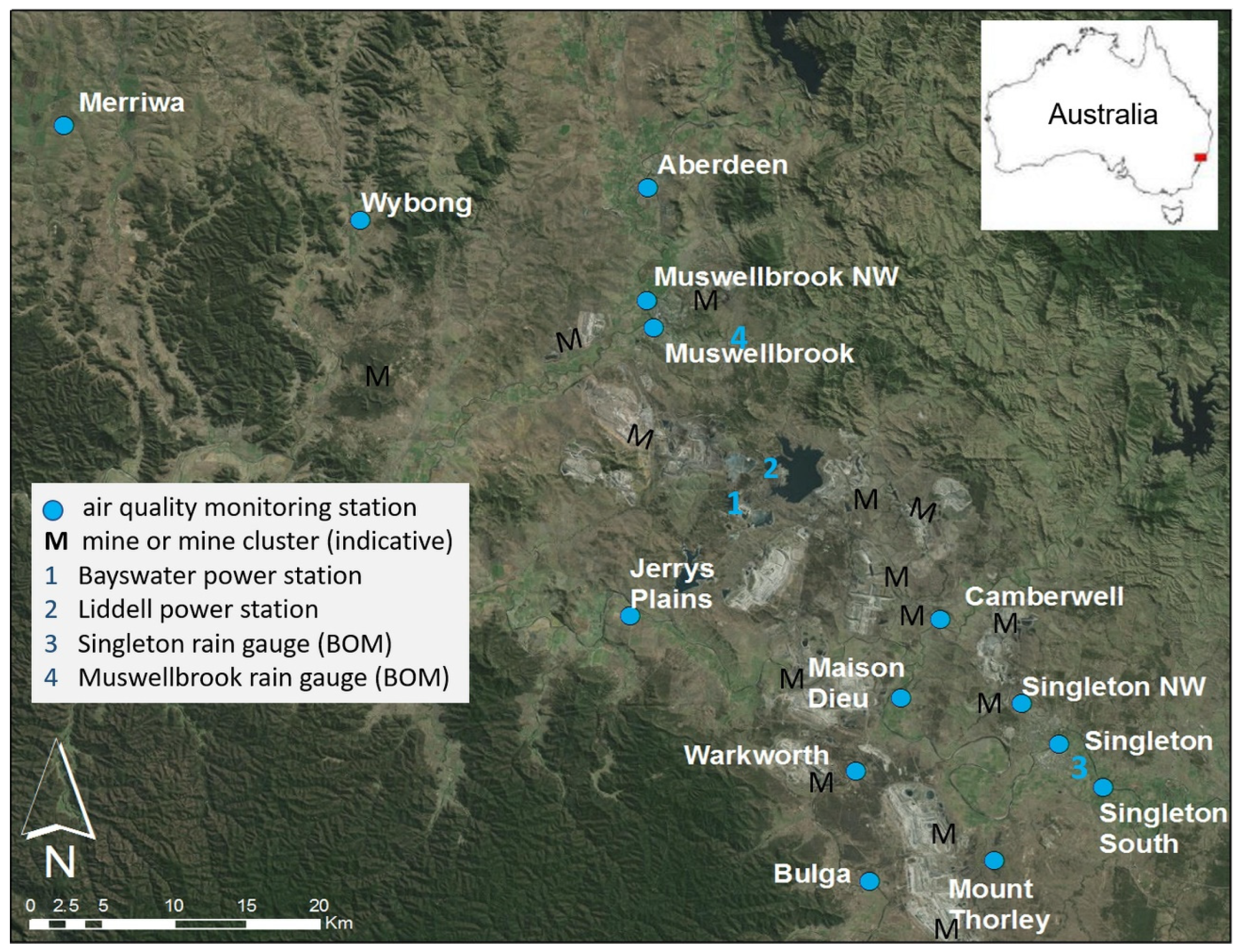
Figure 1.
Upper Hunter Valley—locations of air quality monitoring stations. Red square in the inset of Australian coast lines (top right) indicates the location of the valley. White/grey nuggets on the map represent locations of open-cut mining activities, which have been expanding over time, with “M” labels indicative of current active mine sites or clusters. The Liddell Power Station was decommissioned during April 2022 to April 2023. Source: adapted from Jiang et al. (2024) [3]; base map source: Google.
On a broad scale, the Upper Hunter Valley is oriented northwest–southeast (NW-SE), approximately 30 km wide, and with the terrain elevation estimated in the range of 300–380 m from the bottom (Singleton South) to the top (Merriwa) [3]. On average, PM10 pollution in the region is relatively higher than most other regions in the state [7]. The main sources of PM10 emissions are local open-cut coal mining activities and (wind-blown) surface soil erosion. For example, coal mining contributes around 88% of PM10 emissions in the combined Muswellbrook, Singleton, and Upper Hunter local government areas [8]. Coal-fired electricity generation, agriculture, bushfires, prescribed hazard reduction burnings (HRBs), and state-wide dust storms also contribute to PM10 pollution in the valley. The prevailing surface winds tend to follow the NW-SE orientation of the valley [7,9]. The most frequent winds are north-westerlies in winter and south-easterlies in summer, with wind directions less defined in autumn and spring. Nocturnal and early morning down-valley drainage flows, and daytime up-valley slope winds or sea breezes are observed due to factors such as terrain effects and changes in land/atmospheric heating conditions [10]. The precipitation in the region is low compared to coastal areas to the east, and it varies significantly across years, with higher rainfall in summer and early autumn and lower rainfall in winter and early spring [7,10].
Physical and thermal-dynamic properties of the atmosphere play important roles in determining the level of air pollution over a region through processes such as pollutant generation/emission, transformation, transport, dispersion, and/or deposition/removal [11]. Globally, numerous studies have examined the linkages between meteorological conditions and air quality in urban environments. Most of these highlighted that poor air quality is associated with calm/stable conditions under anticyclonic situations, and good air quality (often) occurs under unstable/cyclonic conditions [12,13,14,15,16]. In addition, a few studies also showed that the passage of low pressure or frontal systems can result in higher particle pollution due to increased soil erosion by wind or transport of pollutants or their precursors [15,17,18,19,20]. In contrast, there are relatively few studies on how meteorological conditions affect the variability of PM10 pollution in rural valley environments. Of those few studies, most researchers relied on the use of correlation analysis and (often short-term) data from selected sites [21,22,23,24,25]. In summary, elevated PM10 pollution in those valleys were associated with (prolonged) dry conditions (low rainfall and humidity), low winds, and/or thermal inversions (low mixing heights), and/or were under the influence of high-pressure systems.
Locally a small number of studies examined the PM10–meteorology relationships in the Upper Hunter Valley. Of these, early investigations were based on short-term campaign monitoring data for selected locations [3]. For example, SPCC (1982) [26] reported the research findings from a few projects, which concluded that dust pollution from open-cut coal mining activities continued to be an issue of concern, and that there was unlikely to be serious (by the then less stringent air quality guidelines) region-wide pollution cumulations resulting from dust emissions from mines. Holmes and Associates (1996) [27] suggested that the increase in dust levels in the valley over 1984–1994 were due to the increase in coal production and the severe drought conditions affecting much of east Australia, and that the land affected by cumulative effects appears to be primarily that owned by the coal mine companies. In contrast, Holmes (2008) and Hyde et al. (1981) [9,28] suggested that local PM10 emissions in the valley can impact air quality in areas away from sources—that is, north-westerlies can transport dust generated in the upper end of the valley to areas near the bottom of the valley or further down over the metropolitan areas of Newcastle. This latter finding appears more consistent with recent air quality monitoring data for the region, for instance, OEH (2017, 2019) and DPE (2022) [5,7,29] reported that PM10 levels in the Upper Hunter Valley were among the highest across the NSW Air Quality Monitoring Network. Based on data in 2012–2015 for 14 stations in the UHAQMN, Jiang (2017) [10] investigated the relationship between a dust (as PM10) risk metric and local meteorological variables using a lagged correlation analysis and the categorisation and regression tree (CART) method. It was found that the correlations between PM10 pollution and individual meteorological variables are complex and non-linear, varying with time and location. Drawing upon this finding, the author recommended that more sophisticated machine learning (ML) techniques such as the Kohonen self-organising map (SOM) method (Kohonen, 2001) [30] can be useful for assessing the impact of weather and climatic conditions on local air quality in the region. The SOM method can be applied for both data classification (structure discovery) and data visualisation (interpretation of results), as was demonstrated in studies for other regions [15,31,32,33].
Till now, to the best of our knowledge, there is little or no research on the topic of quantitatively examining how local and synoptic meteorological configurations combine to modulate the PM10 pollution in valley environments. Jiang et al. (2024) [3] identified the persistent existence of two distinct air quality clusters/subregions in the Upper Hunter Valley and further examined the temporal variability modes of PM10 pollution in these subregions. They found that higher pollution tended to occur in cooler months (late winter to spring) in the southeast (SE) subregion, but in warmer months (especially summer) in the west-northwest (WNW) subregion (also see Section 2.1). The present paper extends the work by Jiang et al. (2024) [3] and other earlier studies [9,28] to report on a quantitative analysis of how elevated PM10 pollution in spring and summer (September to February) of 2012–2022 were associated with typical local and synoptic meteorological configurations over the valley. As noted above, most previous studies on the PM10–meteorology relationship in valley environments relied on the use of correlation analysis and (often) short-term data from selected sites. The present analysis is featured with the visualisation and interpretation of complex results on the SOM planes in a holistic and self-organised manner. The investigation is unique in at least four aspects: (1) a catalogue of 12 synoptic circulation types has been established for the study region for summer and spring seasons, when PM10 levels are generally higher; (2) for the first time, a set of six typical local meteorological patterns has been quantitatively derived for the region for these seasons; (3) the connections between the independently derived local meteorological patterns and typical synoptic circulation types are established and analysed; and (4) the typical synoptic types and local meteorological pattens most conducive to elevated PM10 pollution are holistically identified for two largest population centres, Muswellbrook and Singleton, representing the WNW and SE air quality subregions in the valley, respectively. The methodology and results can be used in air quality research for other locations of NSW, or similar regions elsewhere.
2. Data
2.1. Air Quality Data
Air quality data are available for 14 monitoring stations in the UHAQMN [3]. Based on daily PM10 measurements from these stations, previous studies have identified two distinct air quality subregions in the valley (network)—one in the WNW part, the other in the SE part (Figure 2) [3,10]. Hence, it is possible to characterise (summarise) the air quality variability in the valley with PM10 pollution time series from a subset of (representative) monitoring stations in the subregions [3]. For easy interpretation of results, we chose to focus the present analysis on daily PM10 pollution at stations located at two largest population centres, Muswellbrook (population ≈ 16,357) and Singleton (population ≈ 24,577) [34], representing the WNW and SE air quality subregions in the valley, respectively.
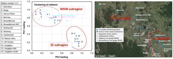
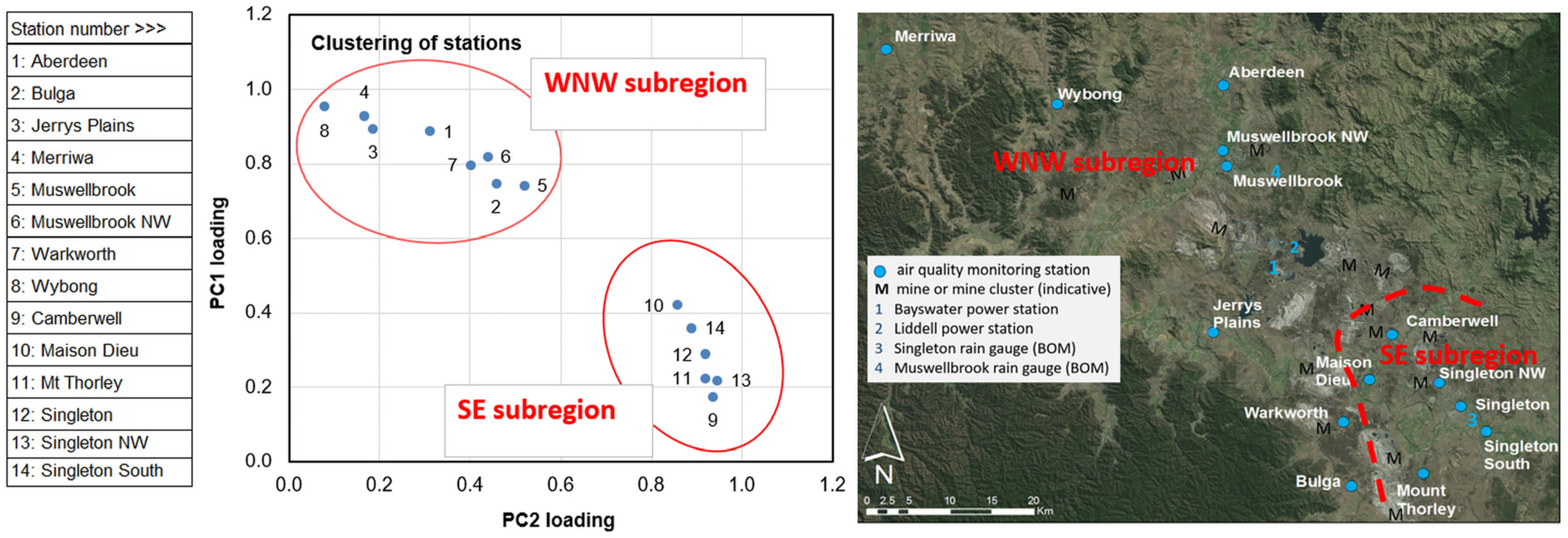
Figure 2.
Identification of two air quality subregions in the Upper Hunter Valley. Left panel: key of station number; middle panel: scatter plot of loadings for first two principal components (PC1, PC2) from Varimax rotated principal component analysis of daily PM10 data (exceptional events excluded); right panel: map showing the UHAQMN stations separated into the WNW and SE subregions. White/grey nuggets areas on map represent locations of open-cut mining activities, which was expanding over time, with “M” indicative of current active mine site or cluster. The Liddell Power Station was decommissioned during April 2022 to April 2023. Source: adapted from Jiang et al. (2024) [3]; base map source: Google.
Air quality data for the Singleton and Muswellbrook stations were obtained from the NSW Air Quality Data System (AQDS) for spring and summer of 2012–2022 (Table 1). These included (1) daily (24 h) average PM10 concentrations (μg/m3) for each monitoring station and (2) information on whether and when PM10 measurements at any of the 14 stations in the UHAQMN were significantly impacted by exceptional events (definition in Section 2.4) such as HRBs, bushfires, or widespread dust storms. The PM10 data were checked and confirmed of high quality, with a small missing data rate (1.6% or less) for spring and summer seasons at both stations.

Table 1.
Details of raw air quality and meteorological data used in this study.
2.2. Local Meteorological Data
Three sets of local meteorological data were obtained for this study (Table 1). One main dataset was obtained from the NSW AQDS for the Singleton and Muswellbrook air quality monitoring stations, including hourly measurements for 10 m horizontal wind, i.e., wind speed (m/s), wind direction (polar degree), and standard deviation of wind direction (SD1; in polar degree), and 4 m air temperature (°C) and relative humidity (%) for 7:00, 13:00, and 19:00 AEST of each day in the spring and summer of 2012–2022. The choice of three-time daily measurements for two stations was to capture (represent) the common diurnal variability patterns in local meteorological conditions across the valley [10]. Wind speed and direction data were used to derive the west–east (u) and south–north (v) wind components, while SD1 records, as indicators of flow direction variability or disturbance, were converted into radians to facilitate the subsequent computations.
The other two datasets included measurements of daily rainfall totals (mm) at two town centres for spring and summer (Table 1). The 24 h rainfall records (previous day 9:00 a.m. to current day 9:00 a.m. AEST) were obtained from the Australian Bureau of Meteorology (BOM) for 2012–2018 at Singleton (station number 061397; 32.59° S, 151.17° E) and for 2012–2022 at Muswellbrook (station number 061374; 32.22° S, 150.92° E) (Figure 1). There were large missing data gaps for the 2019–2022 period, especially at the Singleton station due to site decommissioning. Hence, we also extracted rainfall data from the NSW AQDS for the Singleton and Muswellbrook air quality stations, where rainfall monitoring commenced during late 2016 and early 2017, respectively. For stations located in the same town, there were high correlations between the BOM and AQDS rainfall data for the common period (2016–2018). Hence, the AQDS rainfall data were used to fill in the missing data gaps in the BOM rainfall time series for each site. The improved rainfall dataset was then used to form daily time series for two new variables, indicating soil moisture status and pollution wet deposition process in the valley. The 24 h rainfall record from the previously day 9 a.m. to the current day 9 a.m. AEST was used as proxy variable indicating the soil moisture status in the previous day, since observational soil moisture data were not available at the time of this study. The 24 h rainfall record from the current day 9 a.m. to the following day 9 a.m. AEST was used as weather variable indicating the change in soil moisture (hence potential for dust emissions) and wet deposition process during the current day. This treatment was applied to each site separately, and the resulting dataset for the new variables was combined with the three-time daily meteorological measurements for two air quality stations to form the final local meteorological dataset. The final dataset was used in the SOM classification procedure to quantitatively derive a catalogue of typical local meteorological patterns prevailing in spring and summer (Section 3.1), when PM10 pollution is found to be relatively high.
2.3. Gridded NCEP/NCAR Geopotential Height Data
The data used for the SOM-based synoptic type classification consist of daily 0000 UTC (10:00 AEST) NCEP/NCAR 1000 hPa geopotential height reanalysis for September–February (spring–summer) in 2012–2022 [35]. The study domain covers latitudes 15–50° S and longitudes 130–170° E at a 2.5° × 2.5° resolution, being the same as those used in the previous classifications by Jiang et al. (2015) and Jiang et al. (2017a, b) [15,36]. It is considered sufficient to capture the major synoptic features influencing east Australia.
2.4. Exclusion of Exceptional Events and Definition of Elevated Pollution Days
Jiang et al. (2024) [3] defined exceptional event days as those when air quality in the Upper Hunter Valley was significantly impacted by air emissions from bushfire, planned hazard reduction burning (HRB), and/or continental-scale dust storm, with daily PM10 levels above the 24 h average national benchmark level of 50 µg/m3 [37] at one or more stations in the UHAQMN. We continue to use the definition in this text, so that of the total 1994 days for spring-summer in 2012–2022, there were 111 exceptional event days identified (5.6%). The exceptional event days were excluded from the daily PM10 dataset for further analysis, so that the investigation was focused on PM10–meteorology relationships on non-exceptional event days, i.e., normal days which were impacted mainly by local (within-valley) emissions sources such as coal mining activities and wind-driven soil erosion (as is of most concern in local communities).
The present study was intended to focus on analysing the linkage of meteorological configurations with elevated PM10 pollution in the study region. A day was marked as elevated pollution day if PM10 concentration on that day was above 33.5 µg/m3, i.e., over 67% of the national standard (50 µg/m3) for daily average PM10 levels. This definition led to a derived dataset with only elevated PM10 pollution days for the Singleton (total: 178 days) and Muswellbrook (total: 210 days) air quality stations. The use of data for elevated PM10 pollution days, rather than that for poor air quality (exceedance) days defined by Jiang et al. (2024) [3], was to ensure that the sample sizes are sufficiently large to produce meaningful results from the present analysis. The terms “PM10 pollution” and “air pollution” are used in an exchangeable manner in this text.
3. Methodology
The investigation was conducted in three steps, focusing on the linkage between the occurrence of PM10 pollution on normal days (i.e., non-exceptional event days) with the local- and synoptic-scale meteorological conditions in spring and summer. As noted in Section 2.4, the exceptional event days were excluded from the daily PM10 dataset in the analysis, so that the investigation was focused on understanding the PM10–meteorology relationships on normal days, which were impacted mainly by local emissions sources such as coal mining activities and wind driven soil erosion (which are of most concern in local communities) [3].
In the first step (Section 3.1), we determined the prevailing synoptic and local meteorological features by applying the SOM method to the NCEP/NCAR 1000 hPa geopotential height reanalysis (Section 2.3) and the daily local meteorological dataset (Section 2.2), respectively. In the second step, we examined the connections between synoptic circulation types and local meteorological patterns, based on the classifications resulting from the previous step. The output facilitates the interpretation of results in the third step. The third step was to identify which typical synoptic types and/or local meteorological patterns were most conducive to mean and elevated PM10 pollution in the valley (Section 3.2). For easy interpretation, as noted earlier, the analysis was conducted for two larger population centre stations, Singleton and Muswellbrook, each representing one of the air quality subregions (Figure 2) [3]. The relationships between mean and elevated PM10 pollution and meteorological configurations were holistically visualised and examined on the SOM planes.
3.1. Application of the SOM Technique
There are many classification methods available in the literature [38,39]. Kohonen’s self-organising map, often referred to as SOM in the literature, is one of the most popular neural network methods for unsupervised, non-linear data classification and visualisation [36]. SOM maps the high-dimensional data points (e.g., weather maps) from the input data space onto the nodes (representative patterns, e.g., synoptic types) of a low-dimensional (typically 2-D) grid. In general, SOM mapping can often be conducted in two different ways, through sequential (incremental) or batch training. The two training methods essentially produce the same or similar results, with the batch training converging significantly faster than the sequential training [30]. The batch training method is relatively simple to apply (with no learning rates involved), and it is less sensitive or insensitive to the order of data presentation and map initialisation [40,41].
The utility of a two-phase batch SOM procedure (CP2) for classification of circulation types over east Australia was demonstrated in a few early studies [36,41,42,43]. General details on the implementation of CP2 can be found in Jiang et al. (2012) [42] or Jiang et al. (2015) [36]. In brief, the first phase is to capture a rough estimation of the global structure in the data, and the second phase fine-tunes the mapping to achieve balanced local vs. global optima and thus obtain the final data groupings. CP2 can be run in either data clustering or projection mode—in this study, we applied CP2 in clustering mode, aiming to identify distinctive local and synoptic features influencing the study region. Further details on the CP2 application are given in the following sections.
3.1.1. Classification of Synoptic Types
CP2 was applied to the daily NCEP/NCAR 1000 hPa geopotential height reanalysis for September to February 2012–2022 (Section 2.3) to classify the dominant synoptic circulation types influencing east Australia (including the Upper Hunter Valley). A map size (i.e., total number of nodes/types on the SOM grid) needs to be assigned in the SOM mapping process. We chose to train a 4 × 3 SOM mapping (i.e., 12 synoptic types) from the present dataset, following Jiang et al. (2017a, 2017b) [15]. A geopotential height map was assigned to a SOM node (synoptic type) from which it has the smallest squared Euclidean distance. A synoptic catalogue was then constructed with each day in spring and summer allocated with one of the 12 types on the SOM obtained.
3.1.2. Classification of Local (Within-Valley) Meteorological Patterns
Similarly, CP2 was applied to the local meteorological dataset (Section 2.2) to identify the representative local (i.e., within-valley) meteorological patterns prevailing in the study region during spring and summer. CP2 was implemented on standardised time series, since individual variables were measured in different units, then with de-standardisation applied to the final nodes to obtain the final classification. Several SOM map sizes were considered for the present dataset. Balancing the need for parsimony and variety, the 3 × 2 SOM mapping (i.e., 6 patterns) was found sufficient to reproduce the main meteorological configurations identified in local weather experience [9,10]. Hence, for the first time, a catalogue of six local meteorological patterns was quantitively derived for the study region, with each being interpreted in terms of the combination of individual meteorological variables.
3.1.3. Ordered Visualisation of Complex Results on the SOM Plane
An important property of the SOM mapping is related to the topologically ordered display of the input data in the output space—that is, similar data items from the input space are projected onto the nearby SOM nodes and dissimilar data items onto the SOM nodes further apart. Consequently, the resulting synoptic types (or local meteorological patterns) from the SOM classification are expected to be self-organised/structured on the SOM planes (details in Section 4.1 and Section 4.2). This property facilitates the visualisation and interpretation of the complex meteorology–air pollution relationships on the SOM planes in a structured manner, as was also demonstrated in studies for other regions by Storey et al. (2023), Costa et al. (2022), and Jiang et al. (2016) [31,32,44].
3.2. Air Pollution Tendency Measures
The tendency for PM10 pollution was examined in terms of mean PM10 concentrations and the frequency and propensity for elevated pollution days at the Singleton and Muswellbrook stations, under the occurrence of individual synoptic types, local meteorological patterns, or their combinations.
Mean PM10 levels were calculated as average loadings on each synoptic type or local meteorological pattern. Larger mean values indicate higher overall tendency/potential of the related synoptic type or local pattern for leading to high PM10 pollution in the valley subregions, and vice versa.
Frequency of occurrence for elevated PM10 pollution days was also calculated to reveal how often elevated PM10 pollution events could occur, conditional to the occurrence of individual synoptic types, local meteorological patterns, or the pattern–type combinations. This frequency was expressed as the percentage of days when a local pattern (synoptic type, or pattern–type combination) occurred over the total number of elevated pollution days for the examined station.
The propensity ratio was used to indicate pollution conduciveness of individual synoptic types, local meteorological patterns, or the pattern–type combinations. Following Green et al. (1999) [45], the propensity ratio was expressed as a ratio of the percentage of elevated pollution days for each local pattern (synoptic type, or pattern–type combination) to the overall (climatological) percentage of occurrence of that pattern (synoptic type, or pattern–type combination) in the whole normal-day dataset for spring and summer of 2012–2022. A ratio value greater than one indicates that the local meteorological pattern (synoptic type, or pattern–type combination) is more likely to be present on days of elevated pollution levels than expected. The values of propensity ratios are presented together with frequencies to provide insights into the conduciveness of specific meteorological configurations for leading to elevated PM10 pollution in the valley.
4. Results and Discussion
4.1. Dominant Synoptic Types in Spring and Summer
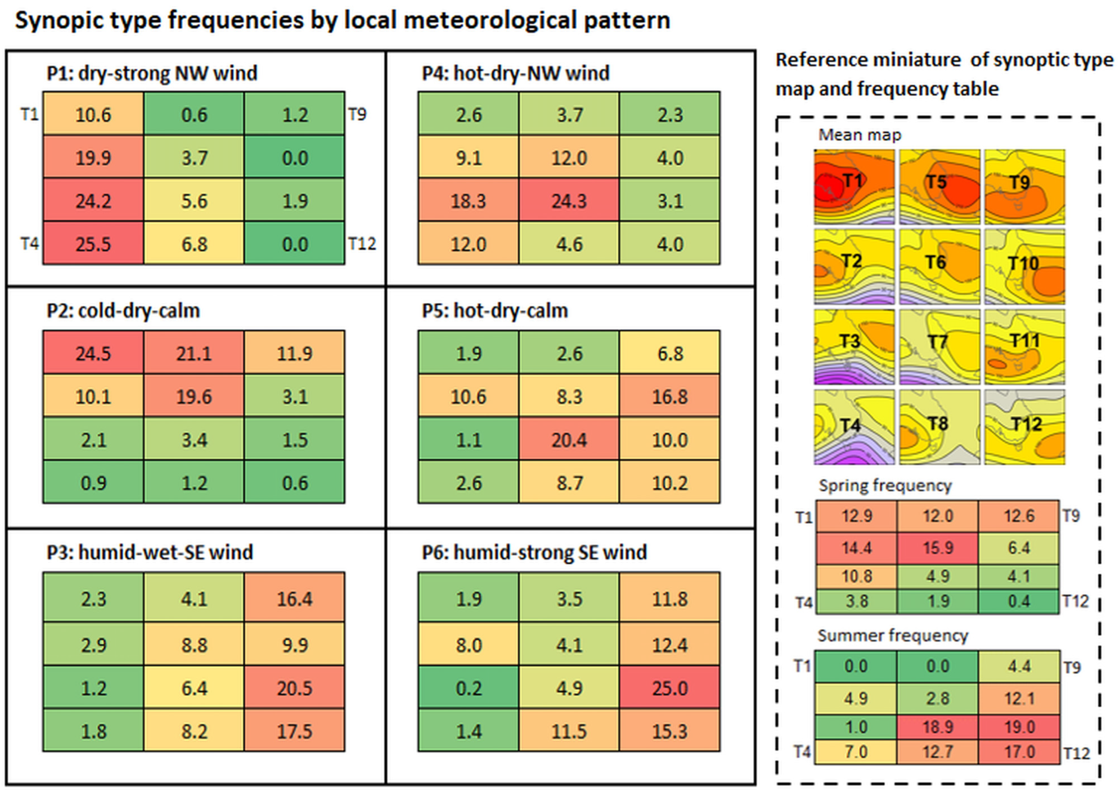
The CP2 (batch SOM procedure) determined a set of 12 synoptic (circulation) types (T1~T12), with similar types close to each other and distinct types further away on the SOM grid/plane, approximating the full spectrum of synoptic states influencing east Australia in spring and summer (Figure 3a). As expected, the classification captures well the interactions among three major synoptic features, i.e., subtropical/continental high, easterly trough/thermal low, and westerly trough/frontal system [46].
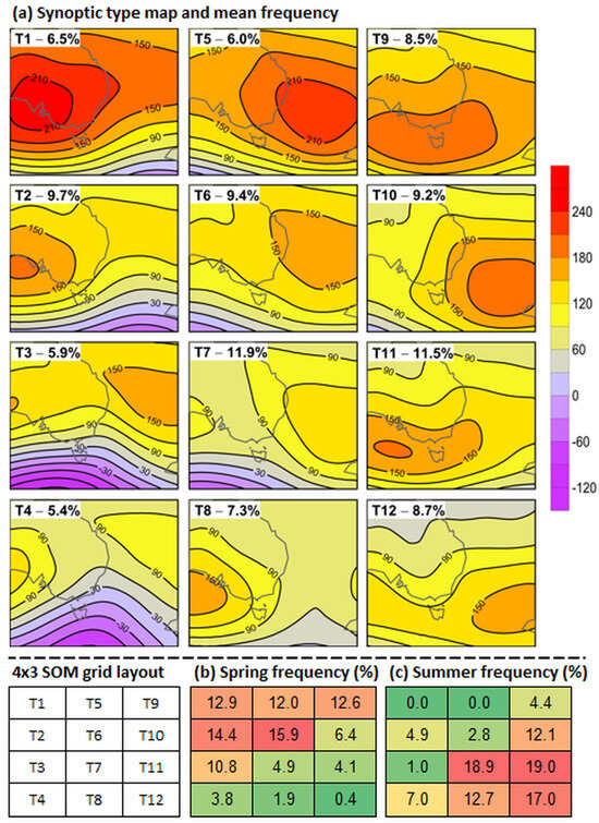
Figure 3.
Synoptic types on the 4 × 3 SOM plane: (a) mean map and frequency of synoptic types T1~T12, where map contours are expressed in 1000 hPa geopotential height (m); (b) spring frequency of T1~T12; (c) summer frequency of T1~T12. Colour scales for (b,c): green—low value; yellow—medium value; red—high value.
On a broad scale, synoptic types near the top-left corner and top edge of the SOM are more frequent in spring (Figure 3a,b), featured with a high system centred over the southern continent near the Australian Bight or a ridge extending northwest from central/northern Tasman Sea towards southern Queensland, as well as the influence of passing westerly troughs (frontal systems) in the further south. In contrast, the situations near the bottom-right corner of the SOM grid show greater prominence in summer (Figure 3a,c), characterised by the influence of a southern high-pressure system (centred over the southern ocean or southern Tasman Sea) and a thermal low/easterly trough system extending southward from northern Queensland. Also of note is that the westerly trough type(s) near the bottom-left corner and the southern high type(s) on the top-right corner of the SOM could occur in both spring and summer (Figure 3b,c). These results are consistent with previous synoptic catalogues for the same region, e.g., by Jiang et al. (2012) and Jiang et al. (2016) for earlier years [42,44].
4.2. Prevailing Local (Within-Valley) Meteorological Patterns in the Upper Hunter Valley
For the first time, a classification of typical local (within-valley) meteorological patterns has been quantitatively derived for the Upper Hunter Valley using the SOM method and based on the long-term data for multiple meteorological variables from the UHAQMN. The classification identified six local meteorological patterns (P1~P6) for the valley, with the mean meteorological conditions for individual patterns being illustrated in Figure 4 and further summarised/visualised on the 3 × 2 SOM grid/plane in Figure 5. Overall, the mean meteorological conditions under each pattern are very similar between two monitoring stations, suggesting that the derived local patterns indeed capture the valley-wide representative conditions. Notably P1~P6 are also topologically ordered on the SOM plane, with distinct patterns located on the opposite corners and more similar ones in the middle section.
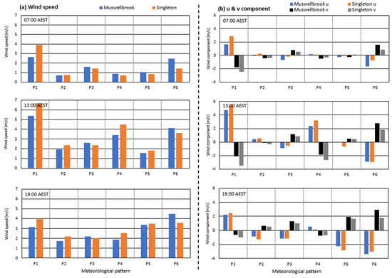
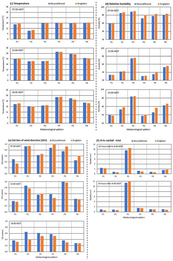
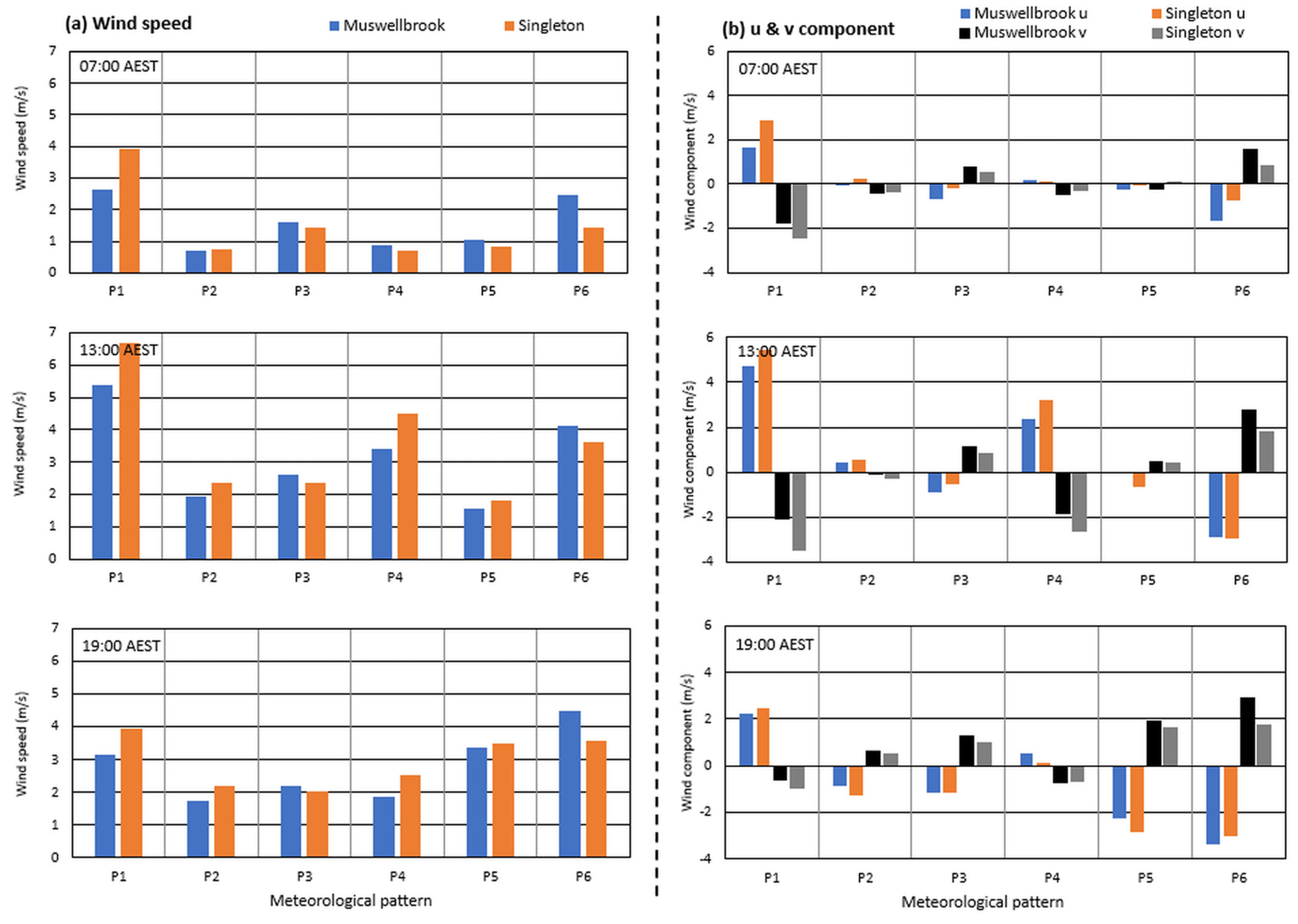
Figure 4.
Mean meteorological conditions at Muswellbrook and Singleton by local meteorological pattern (P1~P6): (a) wind speed; (b) u and v components of wind; (c) temperature; (d) relative humidity; (e) standard deviation (Std Dev) of wind direction (SD1); (f) 24 h total rainfall.

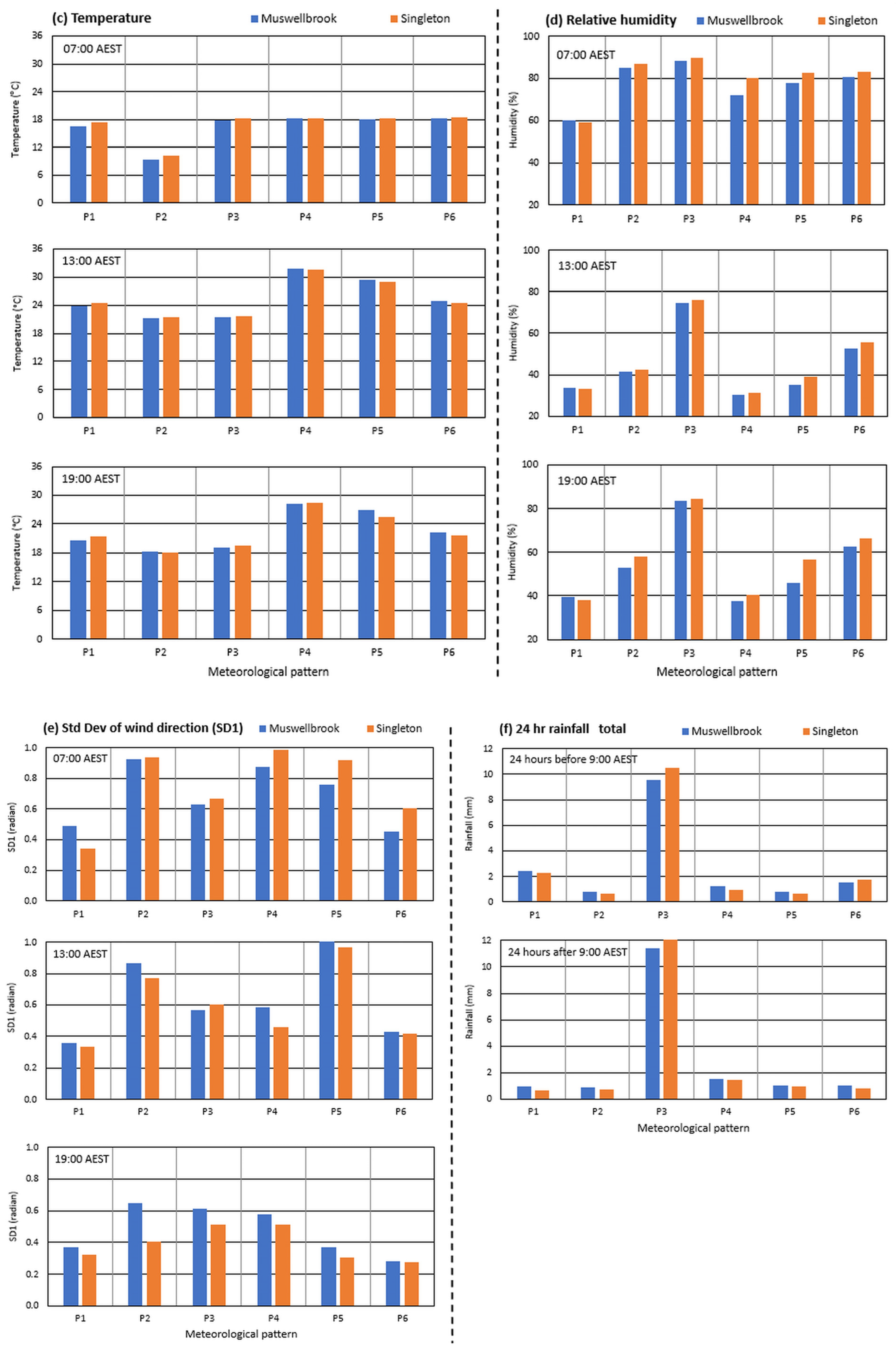
Figure 5.
Local meteorological patterns on the 3 × 2 SOM plane: (a) frequency (%) and description of local conditions for patterns P1~P6; (b) spring frequencies (%) of P1~P6; (c) summer frequencies (%) of P1~P6. Colour scales for (a,b): green—low value; yellow—medium value; red—high value. SE: southeasterly; NW: northwesterly.
The most frequent patterns are P5 (23.6%) and P6 (25.8%), being more prevalent in summer (Figure 4c) and charactered by hot–dry–calm conditions (P5) or humid weather with strong southeasterly (SE) winds (P6). The second most frequent patterns are P2 (16.4%) and P4 (17.6%), with P2 predominantly occurring in spring and P4 equally prevalent in both seasons (Figure 4b,c). These patterns are characterised by (1) cold–dry–calm conditions with potential for night-time or early morning inversion and down-valley drainage flows (P2) or (2) hot and dry weather with prevalence of northwesterly (NW) winds potentially of continental origin (P4). The least frequent patterns are P1 (8.1%) and P3 (8.6%) on the top-left and bottom-left corners of the SOM grid, respectively, typical of dry (and cool) conditions associated with prevalence of strong NW winds (P1) or humid and wet weather associated with moderate SE flows (P3). P1 was more frequent in spring, while P3 was equally prevalent in both seasons.
In summary, all local patterns could occur in spring, with P2 (cold–dry–calm) most prevalent, while P5 (hot–dry–calm) and P6 (humid-strong SE wind) were more often observed in summer. This seasonal difference is somewhat expected due to the seasonal changes in prevailing synoptic circulations described in Section 4.1 and the potential for increased activities of local or meso-scale circulations (such as sea breezes) from spring to summer, as is further discussed in Section 4.3. Overall, the quantitatively derived local patterns reflect the typical meteorological configurations past experienced in the study region, for example, those described in Bridgman and Chambers (1981) and Hyde et al. (1981) [28,47] based on short-term campaign (monitoring) projects, and in Jiang (2017) [10] on the data in 2012–2015 for selected stations from the UHAQMN.
4.3. Linking Local Meteorological Patterns to Synoptic Circulation Types
Early meteorological studies for the Upper Hunter Valley provided generally qualitative descriptions on how local meteorological variables were related to synoptic situations based on short-term campaign monitoring data (Section 1). Here, the connections between local meteorological patterns (Section 4.2) and synoptic circulation types (Section 4.1) can be quantitatively visualised in a holistic framework by taking advantage of the topologically ordered display of the mapping nodes (i.e., patterns and types) on the SOM planes [36]. Figure 6 shows the relative frequency of occurrence for individual synoptic types, conditional to the occurrence of each local meteorological pattern. The main relationships are summarised below:

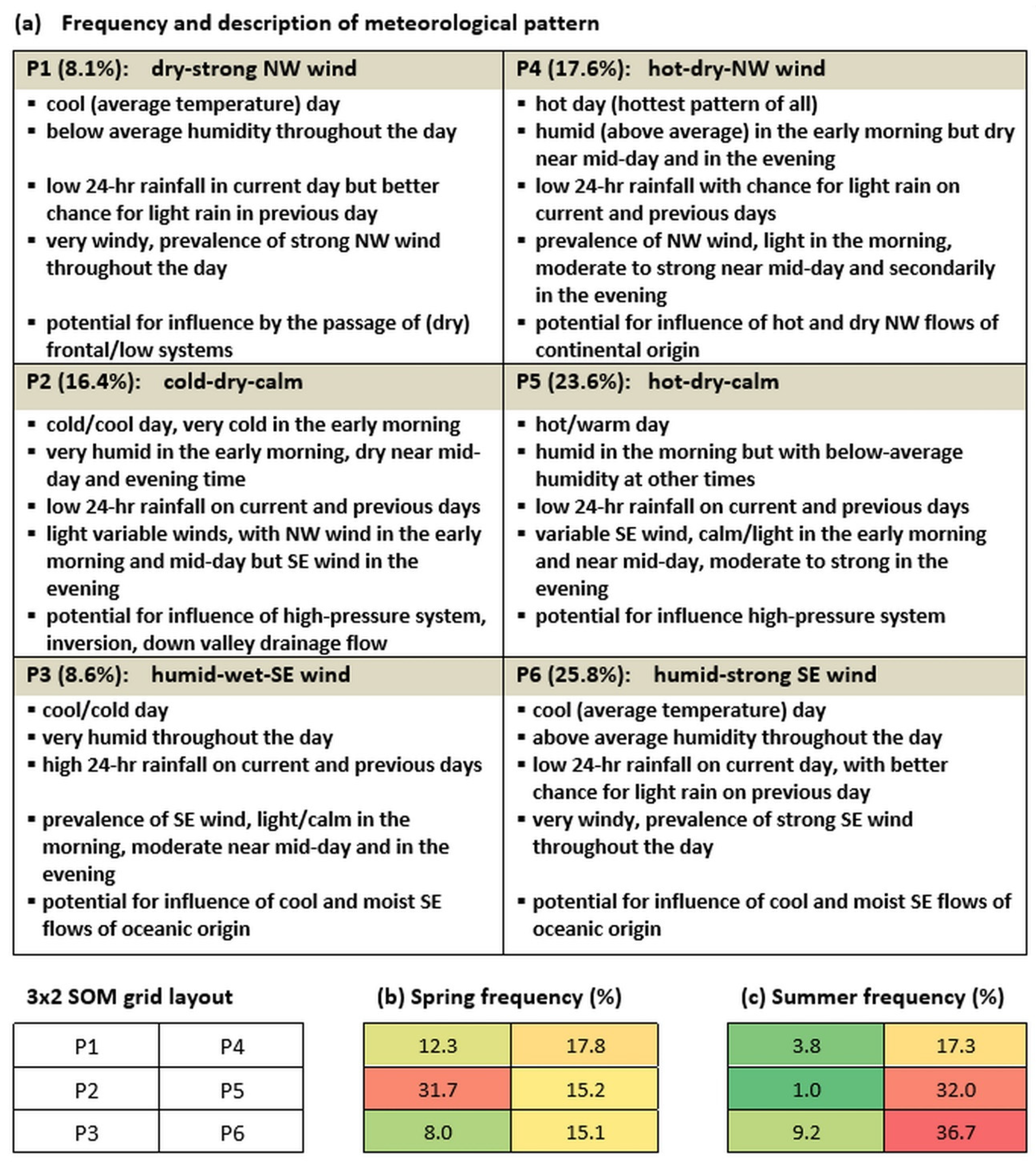
Figure 6.
Linking local meteorological patterns to synoptic types on the SOM planes: relative frequency (%) of 12 synoptic types (T1~T12) on the 4 × 3 SOM grid, under the occurrence of each local meteorological pattern (P1~P6) in September–February displayed on the 3 × 2 SOM grid (boxes on the left two columns). Frequency colour scales: green—low value; yellow—medium value; red—high value. Miniatures of synoptic type maps and frequency tables (details in Figure 3) are given on the right panel (dashed box) for easy reference.
- Local meteorological pattern P1 (dry–strong NW wind) are mostly related to the occurrence of synoptic types T2~T4 and secondarily T1, i.e., anticyclonic/westerly trough types, indicated by relatively high frequencies clustered on the left edge of the 4 × 3 SOM grid. These synoptic states often occur in spring, commonly featured with the influence of eastward migrating continental high and westerly trough, which are often accompanied by the passage of frontal systems over the southern part of the continent [46]. To a much lesser degree, this meteorological pattern is also associated with synoptic types T6~T8, characterised by a high-pressure ridge extending northwest from the central or northern Tasman Sea towards coastal northern NSW or southern Queensland. All these synoptic types tend to provide southwesterly to northwesterly synoptic flows (i.e., flows with westerly components) over eastern NSW, facilitating the prevalence of strong northwesterly winds in the lower boundary layer of the valley.
- Local pattern P2 (cold–dry–calm) corresponds more often to synoptic types T1, T5, and T6, and secondarily T2 and T9, i.e., anticyclonic types, indicated by high frequencies clustered near the top-left edge in the 4 × 3 SOM grid. The synoptic types occur predominantly in spring and commonly characterised by the influence of a strong anticyclonic system over the southern part of the continent or Tasmania, or over the central/northern Tasman Sea, with a potential for providing synoptic-scale light wind or calm conditions over the study region. These situations can lead to anticyclonic atmospheric descending and/or night-time radiative cooling, thus resulting in the occurrence of night-time or early morning planetary boundary layer inversion, down-valley (NW) drainage flows, and/or low early morning ambient temperatures in the region.
- Local pattern P3 (very humid–wet–SE wind) corresponds mostly to the occurrence of T9, T11, and T12, and secondarily T6~T8 and T10, i.e., thermal low/southern high types, indicated by high frequencies clustered near the bottom-right corner and right edge of the 4 × 3 SOM grid. The synoptic states are relatively more often observed in summer, commonly associated with the influence of a thermal low/easterly trough in the northwest and a high-pressure system centred in the south of the domain. These situations can provide synoptic flows with easterly components, broadly facilitating the occurrence of easterly to northeasterly sea breezes over coastal NSW and thus bringing abundant moisture or rainfall over the study region.
- Local pattern P4 (hot–dry–NW wind) corresponds mostly to the situations T7 and T3, and secondarily T2 and T6, i.e., northwest ridge/thermal low types, indicated by high frequencies clustered in the middle to bottom-left sections of the 4 × 3 SOM grid. These synoptic types can occur in both seasons, commonly characterised by a ridge extending towards coastal northern NSW or southern Queensland from the central/northern Taman Sea, a westerly trough in the further south, and potentially a thermal trough extending southward from northern Queensland. These situations can facilitate westerly to northwesterly synoptic flows of continental origin, which transport hot and dry air from inland (central) Australia over the study region, locally with a potential for causing the occurrence of heatwaves.
- Local pattern P5 (hot–dry–calm) corresponds mostly to T7 and T10 and secondarily T2, T6, T8, T9, T11, and T12, i.e., thermal low/southern high/northwest ridge types, indicated by high frequencies clustered near the bottom-right corner of the 4 × 3 SOM grid. These synoptic situations occur most often in summer, commonly characterised by the influence of a thermal low trough extending over NSW from northern Queensland and a high-pressure system centred further south over the (southern) Tasman Sea or near the Australian Bight. These situations tend to provide calm conditions or light northerly to easterly synoptic flows over the coastal regions, resulting in hot, dry, and calm conditions in the valley.
- Local pattern P6 (humid–strong SE wind) corresponds mostly to T11 and secondarily T8~T10 and T12, i.e., thermal low/southern high types, indicated by high frequencies clustered near the bottom-right corner and the right edge of the 4 × 3 SOM grid. These synoptic states occur more often in summer, commonly featured with a thermal/easterly trough in the northwest and a high-pressure system located in south that often manifests coastal ridging effects over the east Australia. These situations often provide synoptic flows with easterly components and to some degree favour the occurrence of easterly sea breezes over coastal NSW, thus leading to the prevalence of strong SE winds in the study region.
Overall, the pattern–type relationships are generally consistent with general meteorological principles for valley environments [46]. In summer, the most prevalent patterns P5 (hot–dry–calm) and P6 (humid–strong SE wind) are more frequently associated with the occurrence of synoptic states featured with activities of southern highs and/or thermal low/easterly troughs, which facilitate anticyclonic low-wind (calm) conditions or the prevalence of easterly synoptic flows over the study region. In spring, the most occurring P2 (cool–dry–calm) corresponds frequently to the occurrence of anticyclonic situations characterised by the influence of high-pressure systems centred over the southern continent or the Tasman Sea. Other pattern–type combinations can also be observed to a lesser/varying degree in this season. It is notable that each local meteorological pattern corresponds to a subset of synoptic types which are somehow similar and clustered together (close to each other) on the SOM plane, and vice versa. Essentially, this non-unique pattern–type correspondence reflects the complexity and subtleness of the interactions between local terrains and atmospheric circulations, which are constantly evolving, rather than existing in a form of discrete clusters. This finding highlights the significant role of local topographical factors in determining the prevailing meteorological conditions in the valley.
4.4. Relation of Synoptic Circulation Types and Local Meteorological Patterns to PM10 Pollution
We examined the linkages between PM10 pollution and the local meteorological patterns and synoptic types identified for spring and summer. As noted earlier, Jiang et al. (2024) [3] suggested that it is possible to characterise the air quality variability in the Upper Hunter airshed with PM10 time series from a subset of (representative) monitoring stations in the air quality subregions (Figure 2; Section 2.1). Here, we chose to analyse the pollution tendency and conduciveness of dominant meteorological configurations in terms of mean PM10 levels and the occurrence of elevated PM10 pollution days at two larger population centre sites, Singleton and Muswellbrook, representing the SE and WNW subregions in the valley, respectively.
4.4.1. Mean PM10 Pollution Levels under Each Local Meteorological Pattern or Synoptic Type
Mean PM10 concentrations are shown in Figure 7, illustrating the overall average tendency of individual synoptic types or local meteorological patterns for contributing to PM10 pollution in the SE and WNW subregions, as represented by the Singleton and Muswellbrook stations, respectively. The clustered patterns of the PM10–meteorology relationships are readily identifiable on the SOM planes. Overall, these relationships are consistent with local air quality experience, for example, those reported in Jiang (2017), Holmes (2008) and Holmes and Associates (1996) [9,10,27] for the Upper Hunter Valley, and in Jiang et al. (2017a) and Leighton and Spark (1997) [15,48] for Sydney.

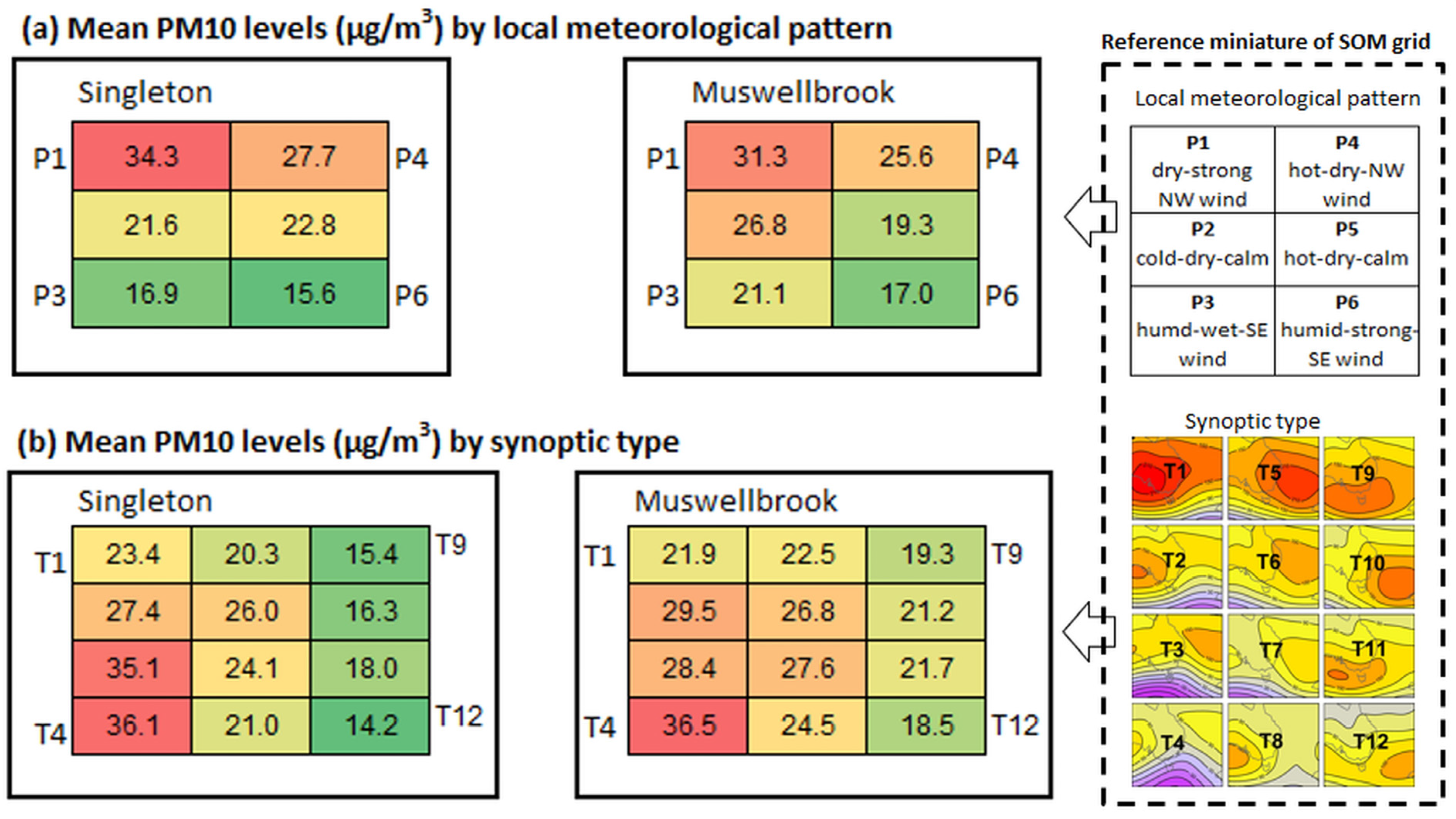
Figure 7.
Mean PM10 concentrations by (a) local meteorological pattern (P1~P6) and (b) synoptic type (T1~T12), displayed on the SOM planes (data for exceptional event days excluded). Colour scale for (a,b): green—low value; yellow—medium value; red—high value. Miniatures of SOM grid layouts with local meteorological patterns and synoptic type maps (details in Figure 5 and Figure 3 respectively) are given on the right panel (dashed box) for easy reference.
Of the six local meteorological patterns, P1 (dry–strong NW wind) and secondarily P4 (hot–dry–NW wind) correspond to much higher mean PM10 levels at both stations (Figure 7a). Local experience suggests that dry NW winds contribute to increased dust generation and down-valley transport of air pollutants, and hence elevated mean PM10 concentrations at the lower part of the valley [10]. Moderately high PM10 levels are observed under P2 (cold–dry–calm) at Muswellbrook and to a lesser degree at Singleton, probably associated with the effect of reduced dust generation (due to suppressed NW wind conditions) confounded by the impact of pollutant accumulation due to low valley ventilations that limit pollutant transport and dispersion. In contrast, P6 (humid–strong SE wind) correspond to the lowest mean PM10 pollution at Singleton and Muswellbrook, since the SE local winds tend to transport pollutants up-slope while also suppressing PM10 accumulation due to high wind speeds (good ventilation).
However, notably, local patterns P3 (humid–wet–SE wind) and P5 (hot–dry–calm) tend to play different roles in determining pollution levels at the two stations (subregions). P3 corresponds to relatively low mean PM10 pollution at Singleton but high mean PM10 levels at Muswellbrook, since the prevailing SE local winds tend to transport pollutants up-slope (away from Singleton, i.e., the SE subregion of the valley), leading to PM10 accumulating near the Muswellbrook area (i.e., the WNW subregion in the upper part of the valley). On the contrary, P5 is associated with relatively high mean PM10 levels at Singleton, but low mean PM10 levels at Muswellbrook, resulting from the effects of reduced dust generation (under suppressed wind conditions) and lack of up-slope pollutant transport (towards the upper end in the WNW subregion), confounded by the impact of pollutant accumulation due to low ventilation conditions. These between-site (subregion) variations in the PM10–local meteorology relationships essentially reflect the significant role of local meteorological conditions in determining the distinct air quality conditions in two subregions, as is suggested by Jiang et al. (2024) [3].
In general, the mean PM10–synoptic type relationships tend to be very similar for Singleton (the SE subregion) and Muswellbrook (the WNW subregion) (Figure 7b). Synoptic types associated with higher mean PM10 levels include T2~T4 and T6 and T7 (highest mean PM10 levels on T4), i.e., those clustered near the bottom-left conner on the 4 × 3 SOM grids, i.e., anticyclonic/westerly trough types and thermal low/northwest ridge types (Section 4.3). These situations are known to provide relatively strong southwesterly to northwesterly synoptic flows over eastern NSW [44], thus facilitating the occurrence of local NW winds in the valley. These relationships are somewhat consistent with the work of Jiang et al. (2017a) [15], who showed that the passage of low pressure or frontal systems, as well as the presence of a high-pressure cell over the Tasman Sea with a ridge extending north-west across NSW or southern Queensland, are commonly associated with elevated PM10 pollution levels and a high chance for exceedance days during warm seasons (November to March) in Sydney.
In contrast, the thermal low/southern high types (T9~T12 on the right edge of the SOM) are related to generally lower mean PM10 concentrations at both stations. This is because these systems often provide mild, moist easterly synoptic flows of oceanic origin (locally in favour of the occurrence of wet weather; Section 4.3) and hence (potentially) resulting in suppressed local PM10 emissions. However, of note are T10 and T11, under which mean PM10 concentrations at Muswellbrook are significantly higher compared to that at Singleton. This is expected, since these southern high/easterly trough types facilitate the occurrence of easterly to southeasterly flows in the study region (Section 4.3), thus in favour of transporting air pollutants from the bottom end (SE subregion) to the upper end (WNW subregion) of the valley. These between-site variations in the low PM10–synoptic type relationships indicate some degree of combined influences from synoptic circulations and local meteorological conditions in discriminating mean air quality conditions in two subregions of the Upper Hunter Valley. This aspect is further discussed in the next two subsections by linking the occurrence of elevated PM10 pollution days at two stations to local meteorological patterns, synoptic types, or the pattern–type combinations.
4.4.2. Occurrence of Elevated Pollution Days under Each Local Meteorological Pattern or Synoptic Type
It is high pollution days that are of most concern in air quality management. In this section, we examine the tendency of individual local meteorological patterns (P1~P6), or synoptic types (T1~T12), for leading to elevated pollution days (events) at Singleton and Muswellbrook. The frequency and propensity ratio values are given on the SOM planes in Figure 8 for P1~P6 and T1~T12, respectively. As noted in Section 3.2, a higher frequency (%) value indicates higher probability for a local pattern (or synoptic type) being observed on an elevated pollution day at the examined station, and vice versa. A propensity ratio greater than one indicates that the relevant local pattern (or synoptic type) is more likely to be present on elevated PM10 pollution days than climatologically expected.
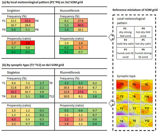
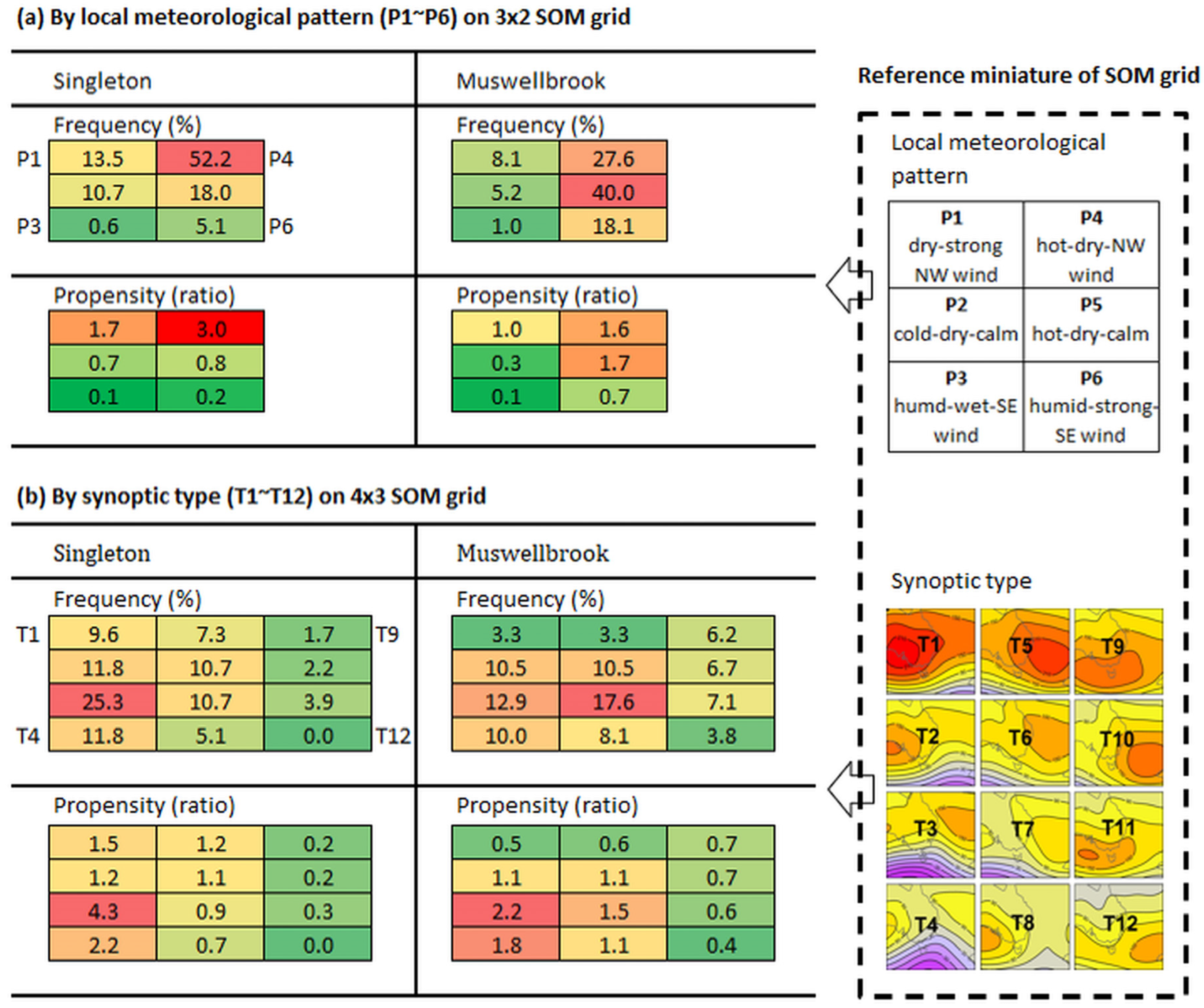
Figure 8.
Linking elevated PM10 pollution days to local meteorological patterns or synoptic types on the SOM plane: frequencies (%) and propensity ratios for (a) local meteorological patterns (P1~P6) on the 3 × 2 SOM grid and (b) synoptic types (T1~T12) on the 4 × 3 SOM grid, for the elevated pollution days (PM10 level > 33.5 µg/m3; exceptional event days excluded) at Singleton (total 178 days) and Muswellbrook (total 210 days). The propensity is expressed as a ratio of the percentage of total number of elevated pollution days to the overall percentage of occurrence for each local meteorological pattern or synoptic type. Colour scale for (a,b): green—low value; yellow—medium value; red—high value. Miniatures of SOM grid layouts with local meteorological patterns and synoptic type maps (details in Figure 5 and Figure 3 respectively) are given on the right panel (dashed box) for easy reference.
Of the six local meteorological patterns (Figure 8a), P4 (hot–dry–NW wind conditions) and P5 (hot–dry–calm conditions) show the highest frequencies (probabilities) for leading to elevated PM10 pollution, accounting for 70.2% and 67.6% of the total elevated pollution days at Singleton and Muswellbrook, respectively. Patterns with moderate probabilities are P6 (humid–strong SE wind; 18.1%) for Muswellbrook and P1 (dry–strong NW wind; 13.5%) for Singleton. In comparison, the propensity ratios illustrate somehow different distribution patterns on the SOM grid. The most pollution-conducive patterns are P4 and P1 for Singleton, but P4 and P5 for Muswellbrook. This highlights a high tendency of the hot–dry–NW wind conditions (P4) for leading to valley-wide elevated PM10 pollution events, with the other two local patterns (P1 and P5) playing different roles for two air quality subregions. As expected, P3 (humid–wet–SE wind), and secondarily P2 and P6, have the lowest propensity ratio values and are thus least conducive to elevated PM10 pollution events among all patterns. Notably the distribution patterns in frequencies and propensity ratios for elevated PM10 pollution events somehow differ from those for mean PM10 concentrations shown in Section 4.4.1. This is an important finding, as it implies that local meteorological configurations tend to play different roles in determining the mean PM10 levels vs. the occurrence of elevated pollution episodes in two subregions.
As shown in Figure 8b, the synoptic types on the centre to left section of the SOM plane are most probably related to the occurrence of elevated PM10 pollution days, with T2~T4 and T6~T7 accounting for a total of 79.8% and 64.8% of elevated pollution days at Singleton and Muswellbrook, respectively. Of these, T3 and T4 have the highest propensity ratios for both sites, hence being commonly pollution-conducive in the two subregions. In addition, relatively high propensity ratios also occur to T1 at Singleton and to T7 at Muswellbrook. These pollution-conducive synoptic types are characterised by the influence of a strong high-pressure system centred near the Australian Bight (T1 and T2), or the passage of a westerly trough or frontal system and a ridge extending northwest towards northern NSW or southeast Queensland from a high centred over the Tasman Sea (T3, T4, T6, T7). In contrast, synoptic types T9~T12, characterised by a high-pressure system centred to the south or southeast of the continent, appear least conducive to elevated pollution days in the valley. In other words, these situations were often associated with relatively better air quality in the valley, more so at Singleton (the SE subregion) than Muswellbrook (the WNW subregion). Overall, synoptic types show similar relationships with the occurrence of elevated PM10 pollution days to that with mean PM10 concentrations discussed in Section 4.4.1.
4.4.3. Occurrence of Elevated Pollution Days Associated with the Local Pattern–Synoptic Type Combinations
The tendency of meteorological configurations for leading to elevated PM10 pollution days is further illustrated in nested SOM grids, as shown in Figure 9 in terms of frequencies and propensity ratios for the local meteorological pattern–synoptic type combinations. In this case, a higher frequency (%) value indicates higher (conditional) probability for a pattern–type combination occurring on (to be associated with) elevated pollution events (days) at the examined station, and vice versa (Section 3.2). Again, a propensity ratio greater than one indicates that the combination is more likely than climatologically expected to be present on days of elevated PM10 pollution. Overall, the combinations of P4 and P5 with T1~T8 appear mostly related to elevated PM10 pollution in the Upper Hunter Valley, with variations observed between two stations (two subregion). The combinations of P1~P3 with synoptic states T9~T10 and secondarily T5~T8 appear least conducive to elevated pollution days.
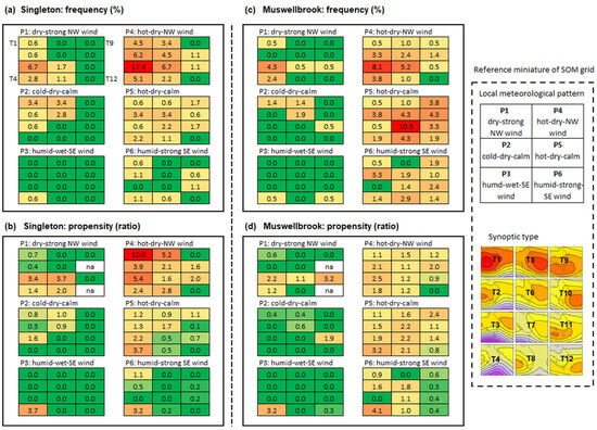
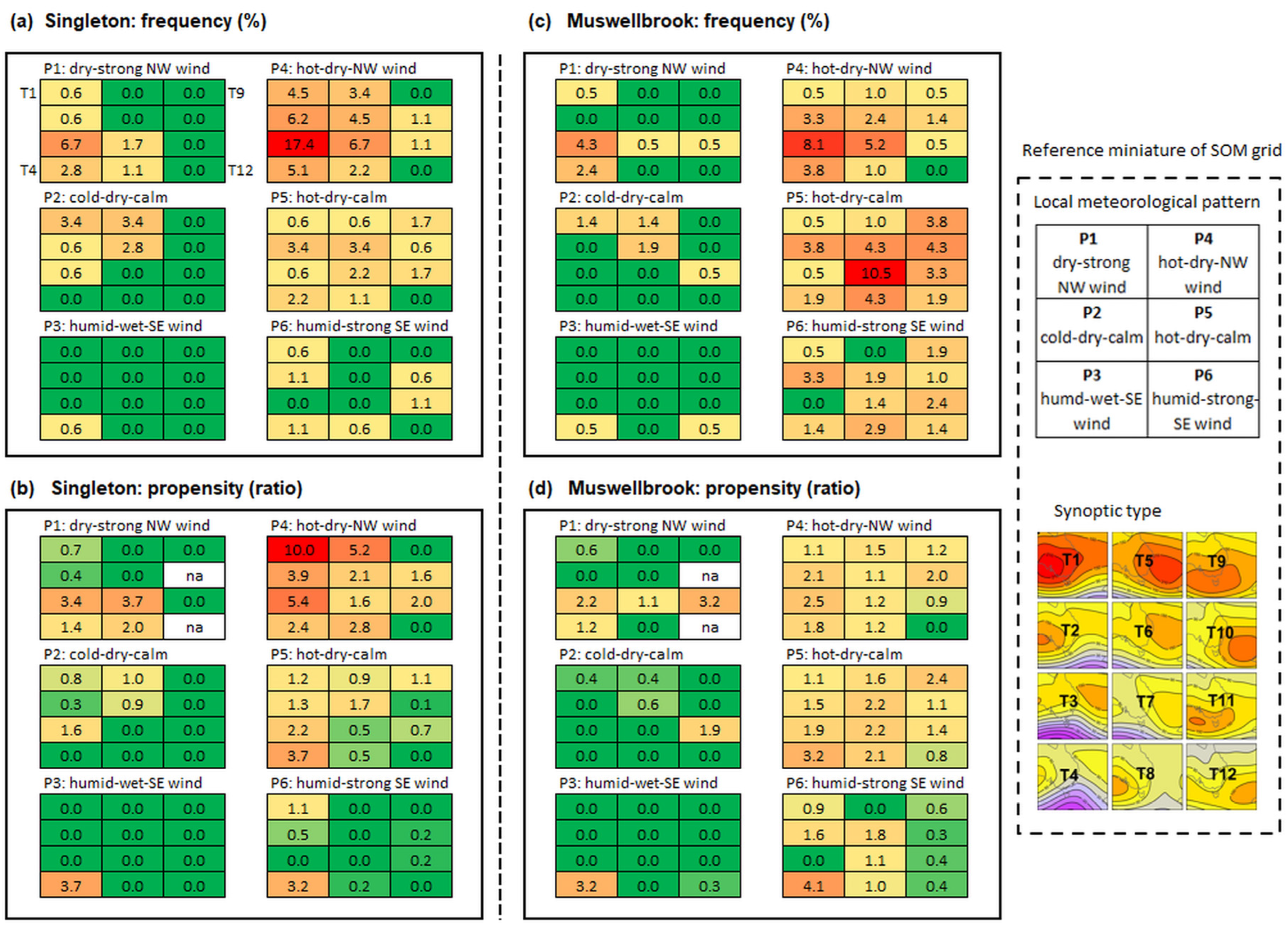
Figure 9.
Linking elevated PM10 pollution to the pattern–type combinations on the SOM planes: frequencies (%) and propensity ratios for each combination of synoptic type (T1~T12) vs. local meteorological pattern (P1~P6) for elevated pollution days (PM10 level > 33.5 µg/m3; exceptional event days excluded) at Singleton (total 178 days) and Muswellbrook (total 210 days). The propensity is expressed as a ratio of the percentage of total number of elevated pollution days to the overall percentage of occurrence for a particular combination of synoptic type–local meteorological pattern. Colour scales for (a–d): green—low value; yellow—medium value; red—high value. Miniatures of SOM grid layouts with local meteorological patterns and synoptic type maps (details in Figure 5 and Figure 3 respectively) are given on the right panel (dashed box) for easy reference.
In particular, the P4 (local hot–dry–NW wind conditions) combinations with T1~ T8, i.e., westerly trough/anticyclonic types or northwest ridge types (Section 4.3), tend to be more pollution conducive. These pattern–type combinations have higher frequencies at the Singleton (total: 50.0%) and secondarily Muswellbrook (total: 25.2%) stations (Figure 9a,c). These combinations are most pollution conducive at Singleton, but to a lesser degree at Muswellbrook, as is indicated by the relatively high propensity ratios (Figure 9b,d). The combinations of P5 (local hot–dry–calm conditions) with synoptic types including T1~T8 also correspond to relatively high occurrence of elevated pollution days, accounting for over 18% and 40% of the total number of elevated pollution days at Singleton and Muswellbrook, respectively (Figure 9a,c). Of these combinations, P5-T4 has the highest propensity ratio and thus is most conducive to elevated pollution days. However, there exist considerable between-site variations, where P5 combinations with T2~T9 appear more pollution-conducive at Muswellbrook but P5 combinations with T1~T4 more pollution-conducive at Singleton (Figure 9b,d).
The P1 (local dry–strong NW wind conditions) combinations with T3 and T4 also have high propensity ratios (thus being pollution conducive) at Singleton and to a lesser degree at Muswellbrook. These synoptic situations are characterised by the passage of westerly troughs or frontal systems, resulting in southerly to southwesterly changes over east NSW and strong northwesterlies (and hence increased dust generations) in the valley. The combinations of P6 (local humid–strong–SE wind conditions) with a few synoptic types such as T6~T12 have relatively high frequencies at Muswellbrook. P6 combinations with T2 and T6 have relatively high propensity ratios (and so are more pollution conducive) at Muswellbrook (in the WNW subregion), while its combination with T4 shows high propensity values (hence being pollution conducive) at both stations (subregions). It is interesting that P3 (humid–wet-SE wind) combined with T4 also shows high propensity ratios at two stations, probably being rare events due to the very low frequencies of this combination (<0.6%).
Hence, the nested display of data on the SOM planes has provided more detailed insights into the relationships between elevated PM10 pollution in the valley and local and synoptic meteorological conditions. These findings are to some degree consistent with overseas studies of PM10 pollution in valley environments, for example, by Mohd Shafie et al. (2022), Quimbayo-Duarte (2021), Reisen et al. (2017), and Giri et al. (2008) [23,24,25,49]. Those studies suggested that elevated PM10 pollution are associated with dry conditions, low winds, thermal inversions, and/or under the influence of high-pressure systems. In addition, the present study has also shown that the passage of westerly troughs or frontal systems, combined with hot and dry local meteorological conditions (i.e., P4 and P5), tend to have high tendency for leading to high mean PM10 levels as well as elevated pollution events in the Upper Hunter Valley. These findings are broadly consistent with the previous studies on the relationship between local and synoptic meteorology and air quality conditions identified for urban environments in NSW. For instance, Jiang et al. (2017a) [15] noted that two synoptic situations, characterised by the presence of a high-pressure cell over the Tasman Sea with a ridge extending north-west across NSW or southern Queensland, are commonly associated with elevated pollution levels and high chance for PM10 exceedance days in the Sydney basin during November–March. As noted earlier, some overseas studies also showed that the passage of low pressure or frontal systems can result in higher particle pollution due to increased wind erosion [17,18].
5. Summary and Conclusions
The present study examined the spatial-temporal variability of PM10 pollution in the Upper Hunter Valley based on the long-term (2012–2022), multi-site air quality and meteorological data. Jiang et al. (2024) [3] reported the findings of the spatial and temporal variation modes by applying rotated principal component analysis and wavelet analysis. This text describes the classification of local meteorological patterns and synoptic circulation types in spring and summer and their relations to mean and elevated PM10 pollution at Singleton and Muswellbrook, representing the SE and WNW air quality subregions in the valley, respectively. The present analysis is featured with the use of the SOM method for the visualisation and interpretation of complex results on the SOM planes, in a holistic and structured manner. The main findings are summarised below:
- (1)
- A catalogue of 12 synoptic circulation types has been established for summer and spring, when PM10 levels are generally higher in the Upper Hunter Valley. The most frequent synoptic types in spring are featured with a high-pressure system centred over the southern continent near the Australian Bight, the influence of westerly troughs/frontal systems in the further south, or a ridge extending northwest towards eastern NSW or southeastern Queensland from a high system centred over the Tasman Sea. In contrast, the more prevalent synoptic situations in summer are characterised by an anticyclonic system located in the south and a thermal low/easterly trough in the north of the domain.
- (2)
- A classification of six local meteorological patterns has been quantitatively derived for the study region for the first time. The classification captures the meteorological configurations commonly experienced in the valley in spring and summer. The two most frequent patterns are (1) hot–dry–calm conditions (23.6%) and (2) humid weather with strong southeasterly winds (25.8%), which can occur in both seasons but more often in summer. The secondarily prevalent patterns are the cold–dry–calm conditions (16.4%), more frequent in spring (rarely occurring in summer), and the hot–dry–NW wind conditions (17.6%), equally frequent in spring and summer. This classification is an important addition to the literature, as most previous studies of the local meteorology–air quality relationships for the region were relatively qualitative or based on correlation analysis of short-term PM10 data and individual meteorological variables.
- (3)
- The connections between local meteorological patterns and synoptic circulation types are quantitatively visualised on the SOM planes for the two independently derived classifications. Each local pattern corresponds to a subset of synoptic types that are relatively similar and clustered together in the SOM grids. In other words, individual local meteorological patterns can have multiple synoptic type counterparts, and vice versa. To some degree, this multiple correspondence may reflect the uncertainty in classifying the continuous, constantly evolving atmospheric states into discrete clusters. However, more importantly, this finding highlights the significant role of the interactions between local terrains and atmospheric circulations in determining local meteorological conditions and consequently air quality in the valley.
- (4)
- Local meteorological pattens and synoptic circulation types are associated with mean PM10 pollution levels for two larger population centre sites (Singleton and Muswellbrook), broadly representing the SE and WNW subregions. On the synoptic scale, higher mean daily PM10 pollution are associated with situations that provide relatively strong southwesterly to northwesterly synoptic flows over eastern NSW. Synoptic types typical of easterly waves with a high-pressure system centred in the south correspond to generally low mean PM10 levels in the valley. Accordingly, two local meteorological patterns, the dry–strong NW wind conditions and the hot–dry–NW wind conditions, correspond to higher mean PM10 levels at both stations (subregions). In comparison, the local pattern featured with cool and humid weather with strong SE winds is related to low mean PM10 pollution in the valley.
- (5)
- There are two groups of local meteorology–synoptic type configurations (combinations) most conducive to elevated PM10 pollution days. One group is featured by the combinations of locally prevailing hot–dry–northwesterly wind conditions in the valley with synoptic situations characterised by (a) the passage of eastward migrating high-pressure systems and westerly troughs (typical of frontal activities) over the southeastern part of the continent (anticyclonic/westerly trough types) or (b) a ridge extending northwest towards coastal northern NSW or southeastern Queensland from the Tasman Sea and a thermal trough extending from the northwest (northwest ridge types). These combinations provide a high chance for leading to elevated PM10 pollution at Singleton (broadly in the SE subregion) and secondarily Muswellbrook (broadly in the WNW subregion). The other group includes the combinations of locally prevailing hot–dry–calm conditions also with the anticyclonic/westerly trough types or northwest ridge types. These combinations have a high chance for elevated PM10 pollution events to occur at Muswellbrook (broadly in the WNW subregion) and to a lesser degree at Singleton (broadly in the SE subregion).
In conclusion, the present study has demonstrated a holistic, quantitative approach for identifying the pollution conducive meteorological configurations for the Upper Hunter Valley. The SOM method has facilitated the classification of both synoptic and local meteorological conditions, and it has also offered the convenience for summarisation and interpretation of the complex results in a structured/clustered manner. The findings have provided further insights into how local- and synoptic-scale meteorological configurations combine to determine the distinct air quality properties in two subregions of the Upper Hunter Valley, as is identified in Jiang et al. (2024) [3].
Our future work may point to a few directions. For example, the findings can be directly applicable for improving air quality data reporting and air quality forecasting [10]. Jiang et al. (2024) [3] identified the variability modes at times scales of 30–90 days and 120 days in PM10 pollution. Previous studies showed that both local-, synoptic-, and large-scale climatic conditions can affect local air quality in a region [19]. Hence, one may speculate whether the PM10 variability modes could be related to the influence of broad-scale climate drivers such as the Madden and Julian oscillation (MJO), El Niño–Southern Oscillation (ENSO), and Southern Annular Mode (SAM), which are known to modulate the weather and climate in Australia—this aspect deserves further attention in future work. In addition, although this study was focused on the air quality–meteorology relationships, it is acknowledged that a detailed analysis on the impact of dust emissions from specific mining sites, when detailed emissions data become available, can also be useful for a more complete understanding of PM10 pollution in the study region. Along this line, the application of coupled meteorology and chemical transport modelling systems, pending the availability of high-resolution terrain (land use) and dust emissions information, may help to shed further light on the complex interactions between local terrain, land use, meteorology, and air quality in the valley environment. Finally, in echo to Jiang et al. (2016) [44], this study has further demonstrated the utility of machine learning techniques for summarising and visualising the air quality data from the NSW air quality monitoring network. The methodology and results from this study can be useful for air quality research at other locations in NSW, or similar regions elsewhere.
Author Contributions
Conceptualisation: N.J.; methodology, data curation and analysis: N.J.; writing—original draft preparation: N.J.; writing—review and editing: N.J., M.L.R., M.A., G.D.V., H.N.D. and P.P. All authors have read and agreed to the published version of the manuscript.
Funding
The Upper Hunter Monitoring Network is funded by local power generation and mining industries in the Upper Hunter Valley and maintained by Department of Climate Change, Energy, the Environment and Water (DCCEEW), New South Wales Government.
Institutional Review Board Statement
Not applicable.
Informed Consent Statement
Not applicable.
Data Availability Statement
The data presented in this study are publicly available at https://www.airquality.nsw.gov.au/air-quality-data-services/air-quality-api (accessed on 8 May 2024).
Conflicts of Interest
The authors declare that they have no conflicts of interest.
References
- Australian Bureau of Agricultural and Resource Economics and Sciences (ABARES). About My Region—Hunter Valley (Excluding Newcastle) New South Wales. 2023. Available online: http://www.agriculture.gov.au/abares/research-topics/aboutmyregion (accessed on 27 September 2023).
- New South Wales (NSW) Minerals Council. Map of NSW Mines. 2024. Available online: https://www.nswmining.com.au/map-of-nsw-mines (accessed on 22 April 2024).
- Jiang, N.; Riley, M.L.; Azzi, M.; Puppala, P.; Duc, H.N.; Di Virgilio, G. Visualising Daily PM10 Pollution in an Open-Cut Mining Valley of New South Wales, Australia—Part I: Identification of Spatial and Temporal Variation Patterns. Atmosphere 2024, 15, 565. [Google Scholar] [CrossRef]
- New South Wales Government. Protection of the Environment Operations (General) Regulation 2021. Available online: https://legislation.nsw.gov.au/view/whole/html/inforce/current/sl-2021-0486 (accessed on 11 October 2023).
- Office of Environment and Heritage (OEH). Better Evidence, Stronger Networks, Health Communities. Five-Year Review of the Upper Hunter Air Quality Monitoring Network; OEH: Sydney, Australia, 2017.
- Riley, M.; Kirkwood, J.; Jiang, N.; Ross, G.; Scorgie, Y. Air quality monitoring in NSW: From long term trend monitoring to integrated urban services. Air Qual. Clim. Change 2020, 54, 44–51. [Google Scholar]
- Department of Planning and Environment (DPE). Upper Hunter Air Quality Monitoring Network, 5-Year Review. 2022. Available online: https://www.environment.nsw.gov.au/research-and-publications/publications-search/upper-hunter-air-quality-monitoring-network-5-year-review-2022 (accessed on 25 March 2023).
- New South Wales (NSW) Environment Protection Authority. 2013 Calendar Year Air Emissions Inventory for the Greater Metropolitan Region in NSW. 2019. Available online: https://www.epa.nsw.gov.au/your-environment/air/air-emissions-inventory/air-emissions-inventory-2013 (accessed on 11 October 2023).
- Holmes. Upper Hunter Valley Monitoring Network Design; NSW Department of Environment and Climate Change: Sydney, Australia, 2008.
- Jiang, N. Upper Hunter Dust Risk Forecasting Scheme Development. Final Report to the NSW Environment Protection Authority; Office and Environment and Heritage: Sydney, Australia, 2017.
- Oke, T.R. Boundary Layer Climates, 2nd ed.; Taylor & Francis: Oxfordshire, UK, 2002. [Google Scholar]
- Lai, H.-C.; Dai, Y.-T.; Mkasimongwa, S.W.; Hsiao, M.-C.; Lai, L.-W. The Impact of Atmospheric Synoptic Weather Condition and Long-Range Transportation of Air Mass on Extreme PM10 Concentration Events. Atmosphere 2023, 14, 406. [Google Scholar] [CrossRef]
- Lee, D.; Kim, H.C.; Jeong, J.H.; Kim, B.M.; Lee, D.S.; Choi, J.Y.; Song, M.Y.; Yoon, J.H. Relationship between synoptic weather pattern and surface particulate matter (PM) concentration during winter and spring seasons over South Korea. J. Geophys. Res. Atmos. 2022, 127, e2022JD037517. [Google Scholar] [CrossRef]
- Salvador, P.; Barreiro, M.; Gómez-Moreno, F.J.; Alonso-Blanco, E.; Artínaño, B. Synoptic classification of meteorological patterns and their impact on air pollution episodes and new particle formation processes in a south European air basin. Atmos. Environ. 2021, 245, 1352–2310. [Google Scholar] [CrossRef]
- Jiang, N.; Scorgie, Y.; Hart, M.; Riley, M.L.; Crawford, J.; Beggs, P.J.; Edwards, G.C.; Chang, L.; Salter, D.; Di Virgilio, G. Visualising the relationships between synoptic circulation type and air quality in Sydney, a subtropical coastal-basin environment. Int. J. Climatol. 2017, 37, 1211–1228. [Google Scholar] [CrossRef]
- Pearce, J.L.; Beringer, J.; Nicholls, N.; Hyndman, R.J.; Uotila, P.; Tapper, N.J. Investigating the influence of synoptic-scale meteorology on air quality using self-organizing maps and generalized additive modelling. Atmos. Environ. 2011, 45, 128–136. [Google Scholar] [CrossRef]
- Dayan, U.; Levy, I. The Influence of Meteorological Conditions and Atmospheric Circulation Types on PM10 and Visibility in Tel Aviv. J. Appl. Meteorol. Climatol. 2005, 44, 606–619. [Google Scholar] [CrossRef]
- Huang, R.; Ning, H.; He, T.; Bian, G.; Hu, J.; Xu, G. Impact of PM10 and meteorological factors on the incidence of hand, foot, and mouth disease in female children in Ningbo, China: A spatiotemporal and time-series study. Environ. Sci. Pollut. Res. Int. 2018, 26, 17974–17985. [Google Scholar] [CrossRef]
- Jiang, N.; Dirks, K.N.; Luo, K. Effects of local, synoptic and large-scale climate conditions on daily nitrogen dioxide concentrations in Auckland, New Zealand. Int. J. Climatol. 2014, 34, 1883–1897. [Google Scholar] [CrossRef]
- Pardo, N.; Sainz-Villegas, S.; Calvo, A.I.; Blanco-Alegre, C.; Fraile, R. Connection between Weather Types and Air Pollution Levels: A 19-Year Study in Nine EMEP Stations in Spain. Int. J. Environ. Res. Public Health 2023, 20, 2977. [Google Scholar] [CrossRef]
- Czernecki, B.; Półrolniczak, M.; Kolendowicz, L.; Marosz, M.; Kendzierski, S.; Pilguj, N. Influence of the atmospheric conditions on PM10 concentrations in Poznań, Poland. J. Atmos. Chem. 2017, 74, 115–139. [Google Scholar] [CrossRef]
- Fortelli, A.; Scafetta, N.; Mazzarella, A. Influence of synoptic and local atmospheric patterns on PM10 air pollution levels: A model application to Naples (Italy). Atmos. Environ. 2016, 143, 218–228. [Google Scholar] [CrossRef]
- Giri, D.; Murthy, K.; Adhikary, P.R. The Influence of Meteorological Conditions on PM10 Concentrations in Kathmandu Valley. Int. J. Environ. Res. 2008, 2, 49–60. [Google Scholar]
- Quimbayo-Duarte, J.; Chemel, C.; Staquet, C.; Troude, F.; Arduini, G. Drivers of severe air pollution events in a deep valley during wintertime: A case study from the Arve river valley, France. Atmos. Environ. 2021, 247, 118030. [Google Scholar] [CrossRef]
- Reisen, F.; Gillett, R.; Choi, J.; Fisher, G.; Torre, P. Characteristics of an open-cut coal mine fire pollution event. Atmos. Environ. 2017, 151, 140–151. [Google Scholar] [CrossRef]
- SPCC. Air Pollution Dispersion in the Hunter Valley; New South Wales State Pollution Control Commission: Sydney, Australia, 1982. [Google Scholar]
- Holmes and Associates. Air Quality Study: Cumulative Effects Due to Atmospheric Emissions in the Upper Hunter Valley, NSW; New South Wales Department of Urban Affairs and Planning: Sydney, Australia, 1996.
- Hyde, R.; Malfroy, H.; Watt, G.N.; Maynard, J. The Hunter Valley Meteorological Study: Interim Report to the New South Wales State Pollution Control Commission on Mesoscale Meteorology in the Hunter Valley; Macquarie University: Sydney, Australia, 1981. [Google Scholar]
- Office of Environment and Heritage (OEH). Annual Air Quality Statement 2018. 2019. Available online: https://www.environment.nsw.gov.au/research-and-publications/publications-search/nsw-annual-air-quality-statement-2018 (accessed on 10 May 2023).
- Kohonen, T. Self-Organizing Maps, 3rd ed.; Springer: Berlin, Germany, 2001. [Google Scholar]
- Costa, E.L.R.; Braga, T.; Dias, L.A.; de Albuquerque, É.L.; Fernandes, M.A.C. Analysis of Atmospheric Pollutant Data Using Self-Organizing Maps. Sustainability 2022, 14, 10369. [Google Scholar] [CrossRef]
- Storey, N.A.; Price, O.F.; Fox-Hughes, P. The influence of regional wind patterns on air quality during forest fires near Sydney, Australia. Sci. Total Environ. 2023, 905, 167335. [Google Scholar] [CrossRef]
- Li, K.; Sward, K.; Deng, H.; Morrison, J.; Habre, R.; Franklin, M.; Chiang, Y.Y.; Ambite, J.L.; Wilson, J.P.; Eckel, S.P. Using dynamic time warping self-organizing maps to characterize diurnal patterns in environmental exposures. Sci. Rep. 2021, 11, 24052. [Google Scholar] [CrossRef]
- Australian Bureau of Statistics (ABS). Search Census Data by Geography—Census. 2021. Available online: https://abs.gov.au/census/find-census-data/search-by-area (accessed on 11 October 2023).
- Kalnay, E.; Kanamitsu, M.; Kistler, R.; Collins, W.; Deaven, D.; Gandin, L.; Iredell, M.; Saha, S.; White, G.; Woollen, J.; et al. The NCEP/NCAR 40-Year Reanalysis Project. Bull. Am. Meteorol. Soc. 1996, 77, 437–472. [Google Scholar] [CrossRef]
- Jiang, N.; Luo, K.; Beggs, P.J.; Cheung, K.; Scorgie, Y. Insights into the implementation of synoptic weather-type classification using self-organizing maps: An Australian case study. Int. J. Climatol. 2015, 35, 3471–3485. [Google Scholar] [CrossRef]
- Australian National Environment Protection Council (NEPC). National Environment Protection (Ambient Air Quality) Measure, Compilation No. 3. 2021. Available online: https://www.legislation.gov.au/Details/F2021C00475 (accessed on 22 June 2022).
- Huth, R.; Beck, C.; Philipp, A.; Demuzere, M.; Ustrnul, Z.; Cahynová, M.; Kyselý, J.; Tveito, O.E. Classifications of atmospheric circulation patterns. Ann. N. Y. Acad. Sci. 2008, 1146, 105–152. [Google Scholar] [CrossRef]
- Philipp, A.; Beck, C.; Huth, R.; Jacobeit, J. Development and comparison of circulation type classifications using the COST 733 dataset and software. Int. J. Climatol. 2016, 36, 2673–2691. [Google Scholar] [CrossRef]
- Vesanto, J.; Himberg, J.; Alhoniemi, E.; Parhankangas, J. SOM Toolbox for Matlab 5. Helsinki University of Technology: Espoo, Finland, 2000; Available online: http://www.cis.hut.fi/projects/somtoolbox/package/papers/techrep.pdf (accessed on 10 December 2023).
- Jiang, N. Application of Two Different Weather Typing Procedures, an Australian Case Study; VDM Verlag Dr. Mueller: Berlin, Germany, 2010. [Google Scholar]
- Jiang, N.; Cheung, K.; Luo, K.; Beggs, P.J.; Zhou, W. On two different objective procedures for classifying synoptic weather types over east Australia. Int. J. Climatol. 2012, 32, 1475–1494. [Google Scholar] [CrossRef]
- Crawford, J.; Griffiths, A.; Cohen, D.D.; Jiang, N.; Stelcer, E. Particulate pollution in the Sydney region: Source diagnostics and synoptic controls. Aerosol Air Qual. Res. 2016, 16, 1055–1066. [Google Scholar] [CrossRef]
- Jiang, N.; Betts, A.; Riley, M. Summarising climate and air quality (ozone) data on self-organising maps: A Sydney case study. Environ. Monit. Assess. 2016, 188, 103. [Google Scholar] [CrossRef]
- Greene, J.S.; Kalkstein, L.S.; Ye, H.; Smoyer, K. Relationships between synoptic climatology and atmospheric pollution at 4 US cities. Theor. Appl. Climatol. 1999, 62, 163–174. [Google Scholar] [CrossRef]
- Sturman, A.P.; Tapper, N.J. The Weather and Climate of Australia and New Zealand; Oxford University Press: Cary, NC, USA, 2008. [Google Scholar]
- Bridgman, H.A.; Chambers, A.J. Air Quality in the Middle Hunter: The Extensive Study Periods. A Report to the New South Wales State Pollution Control Commission; University of Newcastle: Newcastle, Australia, 1981. [Google Scholar]
- Leighton, R.M.; Spark, E. Relationship between synoptic climatology and pollution events in Sydney. Int. J. Biometeorol. 1997, 41, 76–89. [Google Scholar] [CrossRef]
- Mohd Shafie, S.H.; Mahmud, M.; Mohamad, S.; Rameli, N.L.F.; Abdullah, R.; Mohamed, A.F. Influence of urban air pollution on the population in the Klang Valley, Malaysia: A spatial approach. Ecol. Process 2022, 11, 3. [Google Scholar] [CrossRef]

Disclaimer/Publisher’s Note: The statements, opinions and data contained in all publications are solely those of the individual author(s) and contributor(s) and not of MDPI and/or the editor(s). MDPI and/or the editor(s) disclaim responsibility for any injury to people or property resulting from any ideas, methods, instructions or products referred to in the content. |
© 2024 by the authors. Licensee MDPI, Basel, Switzerland. This article is an open access article distributed under the terms and conditions of the Creative Commons Attribution (CC BY) license (https://creativecommons.org/licenses/by/4.0/).