Abstract
Growing global concern over greenhouse gas emissions has led to a demand for understanding and addressing carbon emissions, with China being one of the main contributors to global carbon emissions, committed to reach the carbon peak by 2030. As a result, much previous research has delved into the drivers of carbon emissions in China; however, few studies have included new energy factors in the extended STIRPAT model when analysing the data, employed more advanced visualisation techniques such as force-directed diagrams, and explored factors outside of the industrial and energy sectors in determining China’s ability to reach their environmental goals. In this study, we use the extended STIRPAT model to analyse a more diverse range of drivers for carbon emissions in China and discuss methods to reach peak carbon emissions through the implementation of environmental policies. Using data from China’s 14th Five-Year Plan and Vision 2035 to set up two simulation scenarios, we predict China’s carbon emissions, introducing ridge regression to ensure validity, and employing big data and visualisation techniques to aid in interpreting results. Our findings suggest that China needs to implement more stringent environmental policies to meet its commitment to reach peak carbon emissions by 2030, revealing that factors such as per capita arable land area, per capita GDP, the proportion of people living in extreme poverty, the level of tourism development, the use of fossil fuels, and new energy technologies have a significant impact on China’s carbon emissions. As such, we can recommend more stringent policies relating to the agricultural, energy, and tourism sectors to help China achieve their goal of carbon peak by 2030.
1. Introduction
As global warming progresses, more and more countries worldwide have become increasingly concerned about greenhouse gas emissions, with one of the most significant contributors being carbon dioxide emissions. Globally, China is considered one of the countries most vulnerable to climate change, global warming, and environmental degradation. China is ranked 120th out of 180 countries in the 2020 Environmental Performance Index (EPI) ranking. In response to environmental pressures, China’s leaders have pledged to reach peak carbon emissions by 2030 and become carbon-neutral by 2060 [1,2,3,4].
Currently, research on China’s carbon emissions primarily focuses on the energy and industrial sectors, and this is due to the establishment of a large variety of different studies that heavily link carbon emissions with the energy and industrial sectors, especially in their extensive use of fossil fuels.
The use of fossil fuels has had extensive links to pollution, as shown by various past studies:
- Lin et al. (2018) collected data on factors such as sub-micron aerosols (PM1) for Ireland from 2016 to 2017, used a sophisticated fingerprinting technique to determine the proportion of peat and wood consumed, identified them as the main contributors to air pollution due to the combustion of solid fuels [5].
- Hanif (2018) examined a panel of 34 emerging economies in sub-Saharan Africa with panel data from 1995 to 2015 using the systematic generalised method of moments (GMM), highlighting the significant contribution of fossil fuel consumption and urban sprawl to CO2 emissions [6].
From China’s 14th Five-Year Plan and Vision 2035 plan, there is a focus on an increase in high-value invention patents and GDP, as well as binding regulations on fossil fuel consumption and air pollution indices, which provide some indication of future carbon emission scenarios. GDP per capita and agricultural land per capita can reflect the level of economic development and land use, and tourism represents the structural transformation of the economy and may have some relevance to carbon emissions [7]. These plans also highlight the issues of poverty reduction and population growth, factors that may also influence carbon emissions [8].
These areas of focus, however, seem to be less studied, potentially hindering the ability to comprehend the complex effects that these areas have on carbon emissions, particularly with the development of new energy technology and environmental sustainability and their relationship with carbon emissions in China [9,10,11,12,13]. This highlights a potential knowledge gap in policymaking concerning greenhouse gas emissions in China.
This gap in knowledge can be partially bridged through contemporary research:
- Nabi et al. (2020) conducted a study on 98 developed and developing countries for the year 2011 using cross-sectional and transformed regressions. It was found that poverty indirectly affects carbon emissions. This view is supported by Benedikt Bruckner (2022), who studied the eradication of poverty in 116 countries, including the United States, and found that a reduction in carbon emissions is closely related to a reduction in poverty [14,15]. This suggests that there seems to be a link between poverty reduction and carbon emissions, and we would like to extend this link by looking at the scope of Ikuna’s carbon emissions, especially given China’s poverty alleviation programme.
- The study by Tian Xianliang (2021) collected panel data on CO2 emissions, renewable energy consumption, GDP, and number of tourists for 19 G20 economies from 1995 to 2015, tested the data for cointegration using seven methods, including Pedroni’s test and Kao’s test, and extracted the data using the FMOLS method. The results indicate that tourism development contributes to carbon emission reduction [16], which indicates another factor to be further explored through the Chinese context.
While these studies have improved our understanding of policy scenario projections and associated carbon emission drivers, to the best of our knowledge, several limitations constrain the development and application of the concepts [17,18]. There presently seems to be a lack of research on the direct correlation between the development of new energy technologies, the share of people living in extreme poverty, air pollution from solid fuel combustion, and carbon emissions, an issue exacerbated by the fact that research into the various drivers of carbon emissions has mainly focused on energy intensity, energy mix, and industrial structure, with a lack of focus on the development of new energy technologies, solid fuel combustion, agriculture, and tourism.
These potential gaps in knowledge combined with a lack of research in determining whether or not China is able reach its goal of achieving a carbon peak by 2030 given its outlined policies in the most recent 14th Five-Year Plan and Vision 2035 plan, to the best of our knowledge, present an area for our study to target.
In analysing environmental factors, we found the STIRPAT model, standing for stochastic effects of population, affluence, and technology regression, to be a commonly chosen model in determining the impact of human activities on environmental pressures, particularly in carbon emissions [17], with Ma et al. (2017) employing the STIRPAT model to assess the drivers affecting carbon emissions from existing public buildings in China from 2000 to 2015, demonstrating its prevalence even in a Chinese context [19].
The model exists as an environmental assessment tool, first proposed by Ehrlich and Holdren in 1974, with a broad range of applications in various fields, such as environmental impact assessment, climate change research, sustainable development, energy policy and planning, and urbanisation and the environment, providing a powerful means of understanding environmental issues and guiding decision-making [20,21,22].
Due to its simple and flexible structure, a derivation of this STIRPAT model can be formed to use linear regression to identify the stochastic impacts of these factors. We identify this derivation as the extended STIRPAT model, which will be further explained in the method. This extension of the model allows for more effective integration of the various complex multivariate relationships of the carbon emission problem, displaying a stronger ability to analyse complex, nonlinear relationships in environmental data analysis [23].
This extended version of the STIRPAT model was used to investigate the drivers of carbon dioxide emissions in China [18], demonstrating a precedent in the use of the extended model in the environmental analysis of China.
We believe that the extended model’s reliability and scalability make it strong, enabling a comprehensive assessment of issues such as environmental change and carbon emissions, especially considering the potentially complexity of the relationship between the various sectors of development and carbon emissions in China.
However, as the prerequisite for establishing a regression model is that the dependent variable satisfies a normal distribution, to use the extended model in more complex datasets, we would require the validation of our input data to ensure that they are fit for use for the extended STIRPAT model [24].
To help validate the dataset and to ensure that the data can be analysed in a linear regression analysis using the extended STIRPAT model, we found that the ADF test (the augmented Dickey–Fuller test), Johansen’s test of cointegration, and the VIF method (variance inflation factor) of factorial independence can be used [25].
Correlation between variables can be analysed through the Spearman correlation analysis, presenting as a more robust correlation method and one that is insensitive to outliers, being more widely applied and not subject to the limitations of the linear relationship [26].
Ridge regression represents the best choice in regression analysis as it can assist in addressing multicollinearity issues, which may arise due to the complex dataset that this study aims to analyse, mitigating covariance through introducing a regularisation term, and effectively controlling the magnitude of parameter estimates by imposing penalties on the coefficients [27].
In representing the results obtainable from the extended model, visualisation techniques allow for the easiest interpretation of data, allowing for a better understanding of potential correlation between variables, with force-directed diagrams presenting as one of the major visualisation techniques that allow for the simple graphical interpretation of data [28,29,30,31].
From the limitations of prior research to the best of our knowledge, and considering China’s goals of poverty eradication, tourism, agriculture, and the development of new energy technologies, from China’s Vision 2035 plan and the commitment to reach peak carbon by 2030, we selected 12 factors to plot against China’s annual CO2 emissions: GDP per capita, the proportion of people living in extreme poverty, electricity generation from fossil fuels, deaths due to air pollution caused by solid fuels, per capita land used for agriculture, and that for tourism, thermal energy storage technology, battery technology, electric vehicle mechanical technology, electric vehicle storage technology, electric vehicle management technology, and electric vehicle charging pile technology. Two carbon emission reduction scenarios can be derived based on China’s 14th Five-Year Plan and Vision 2035: the standard baseline scenario (FBU) and the green scenario with stricter environmental policies (SBU). We believe that through analysing these factors through the lens of these two scenarios, using data from 2002 to 2023, we will be able to aid in bridging the knowledge gap that currently exists in the analysis of China’s carbon emissions, exploring the paths leading to sustainable development by alleviating carbon emission concerns through discovering insights with various less researched contributors to China’s carbon emissions, accurately determine and project China’s carbon emissions to determine their ability to reach their environmental goals, and be able to offer novel policies to Chinese policymakers to help reach China’s carbon emission targets.
Based on these two scenarios, the findings of past studies, and our selected factors, four hypothesises can be derived:
Hypothesis 1 (H1).
In the baseline scenario, the long-term relationship between GDP per capita and carbon emissions in China satisfies the EKC theory [6].
Hypothesis 2 (H2).
Fossil fuel power generation has the largest positive driving influence on China’s carbon emissions.
Hypothesis 3 (H3).
The development of new energy technologies will ease pressure on China’s carbon emissions.
Hypothesis 4 (H4).
China can meet its Peak Carbon Commitment by 2030 under the baseline scenario.
Through careful analysis of various datasets with a variety of appropriate techniques informed by the contemporary literature, we will attempt to substantiate these hypotheses to alleviate the limitations of past studies as well as generate suggestions for policymakers to help carbon emissions in China.
Figure 1 shows the research framework, to provide a clearer outline of how our research was carried out.
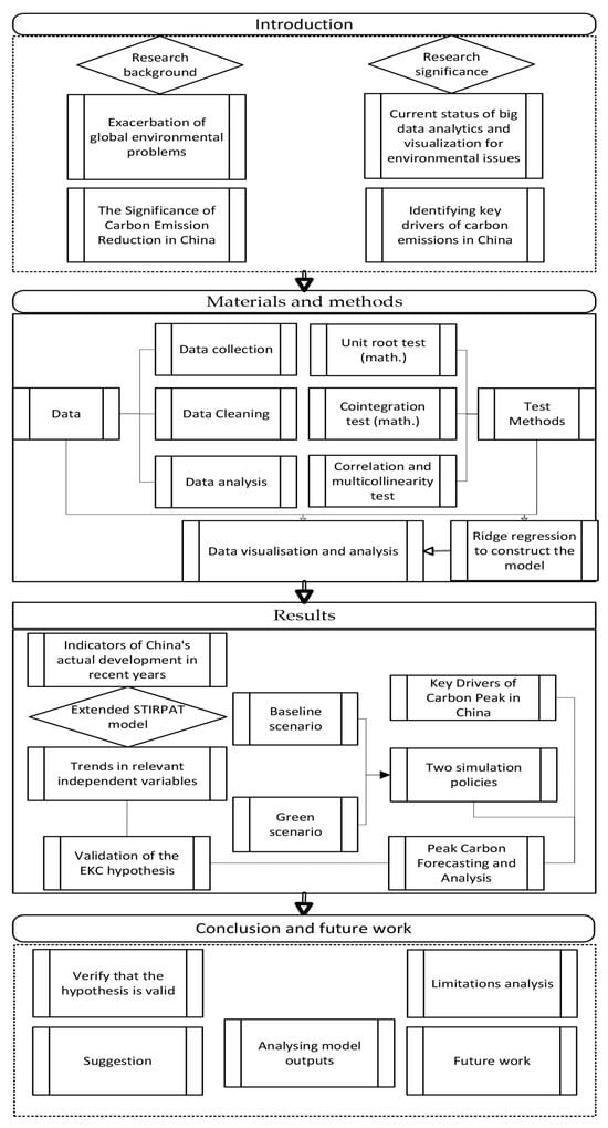
Figure 1.
The research framework and procedures of the study.
2. Materials and Methods
Our research methodology included data collection, cleaning, and analysis.
We obtained data from eight publicly available official datasets that are closely related to the themes and questions of the study. This was carried out as public datasets have a higher degree of accessibility and transparency, which helps other researchers to validate and replicate findings and ensures that the findings are widely applicable. Moreover, these data are released by government departments, international organisations, or authoritative bodies, which have a high degree of authority and credibility, and such data sources are more likely to be subject to stringent quality control and monitoring, thus reducing the likelihood of data errors or manipulation. At the same time, these datasets are largely complete and have low data gaps, reducing the impact of data bias.
We collected data relating to the number of patent applications in the field of new energy in China in recent years from the International Renewable Energy Agency (IRENA) [32] and the Energy Research Institute (ERI) [33], the proportion of the population living in extreme poverty in China from the World Bank’s database [34], China’s carbon emissions from the Global Carbon Project [35], GDP per capita and annual tourist arrivals from the database of the National Bureau of Statistics (NBS) [36], fossil energy power generation from Ember [37], Agricultural land per capita from the Food and Agriculture Organisation of the United Nations (FAO) [38], and population deaths due to solid fuel combustion from the World Health Organisation [39].
To handle this extensive dataset, we utilised the “Web Scraper” tool for data crawling. We established filtering criteria within Web Scraper, enabling precise data extraction and the exportation of the selected data [40,41]. To ensure data reliability, we employed the culling method of identifying and subsequently removing outliers to minimise the impact on data analysis and modelling [42].
The basic idea of the culling method is to identify and remove outliers from the data set to reduce their impact on data analysis and modelling, employing a threshold-based approach, setting reasonable threshold ranges based on the actual meaning and context of each feature, considering data that exceed these threshold ranges as outliers, and flagging them for further processing. For example, we found that the proportion of extremely poor people in China in 2003 was a null value, and we eliminated it.
The abbreviations used in this study concerning the drivers we analysed are shown in Table 1.

Table 1.
Abbreviations used in this article.
We then used Tableau to plot long-term trends using the 12 outlined variables. These trend graphs were plotted to help one understand the evolutionary trends of these variables as a whole and to identify early on which variables may be more important than others.
In mapping these trends, we first collected relevant data between 2002 and 2020, cleaning and organising the data. Next, we performed the necessary aggregation, filtering, and grouping operations on the data to better present the relationships and trends among the variables. In terms of chart design, we considered factors such as colours, labels, and line styles to ensure that the charts were clear and easy to understand and that they accurately conveyed the evolution of the variables.
The final trend graph shows the trend of the 12 variables between 2002 and 2020, allowing observers to visualise the evolution of these variables and identify trends that may be significant.
Next, we conducted a Spearman correlation analysis on 12 variables, including ACO2, pairwise. The Spearman correlation coefficient, a non-parametric indicator ranging from −1 to 1, reflects the strength and direction of correlation. Negative coefficients closer to −1 indicate a stronger negative correlation, while positive coefficients closer to 1 denote a stronger positive correlation. Values closer to 0 suggest a weaker correlation, with the method being robust across various data distributions and insensitive to outliers [43,44,45].
After analysing the correlations among variables, we summarised the Spearman correlation coefficients and generated correlation heatmaps using Python code. Additionally, we plotted correlation force-directed graphs between variables using Gephi.
Our force-directed graphs utilise a force-directed layout algorithm, simulating nodes in the graph as atoms based on particle physics theory. By modelling the force field between atoms, we derive the positional relationships between nodes. This algorithm accounts for gravitational and repulsive forces between atoms to calculate node velocity and acceleration, akin to the laws governing atomic or planetary motion, ultimately reaching dynamic equilibrium [46].
We then carried out a linear regression analysis to provide a clearer picture. Linear regression analysis is a statistical method that helps us understand the relationship between the independent and dependent variables. This type of analysis quantifies the effect of the independent variable on the dependent variable, identifies the key factors that affect the dependent variable, and predicts the trend of the dependent variable. In addition, by looking at the regression coefficients and significance levels, we can determine which variables have the greatest explanatory power for the model and the overall fit of the model. In addition, linear regression analysis can reveal underlying patterns and trends in the data, providing valuable insights for relevant decision-making and strategy development.
We used the small sample normality test and Shapiro–Wilk test to assess the normality of ACO2. A p-value greater than 0.05 indicates that the data conform to a normal distribution and that the normality plot shows a symmetrical distribution of the data, which suggests that the dataset meets the requirements for conducting linear regression analyses.
Then, to ensure the reliability of the input data, the ADF (Augmented Dickey–Fuller) test was used to examine the stability of the independent variables [47]. The test is based on the principle of determining whether or not there is a unit root in the data series. If the variable has a p-value of <0.05, the ADF test considers it a smooth series.
To avoid the problem of pseudo-regression, we conducted a cointegration test on the two unsteady series. We used the Johansen cointegration test method as it is more interpretable for independent variables compared with the Engel–Granger (EG) cointegration test method [48,49]. Based on the Johansen cointegration test interpretation, if the trace statistic exceeds the 1% critical value, the current hypothesis is rejected. The results of Johansen’s cointegration test are shown in Section 3.
To prevent the impact of multicollinearity on the regression equation, we assessed the correlation coefficients and variance inflation factors (VIF) of the 12 variables included in the model.
Multicollinearity detection involves checking for a VIF (variance inflation factor) greater than 10, which indicates the presence of multicollinearity between variables. A VIF greater than 100 indicates severe multicollinearity. The use of OLS regression, which is widely used in this study, may not be appropriate if severe multicollinearity exists in the dataset. Instead, ridge regression is a more appropriate choice. OLS regression (ordinary least squares regression) may lead to unstable or even unexplained coefficient estimates in the presence of multicollinearity.
Ridge regression, on the other hand, solves the problem of multicollinearity by introducing regression terms, thus improving the stability and generalisation of the model. In ridge regression, by controlling the ridge parameter (regularisation parameter), the effect of multicollinearity on coefficient estimation can be reduced, resulting in more reliable and robust results. Therefore, we chose ridge regression as the analytical method to ensure the accuracy and reliability of the model.
After verifying that the dataset is fit for linear regression, we used a derivation of the STIRPAT model.
The STIRPAT model can be expressed in equation form as follows:
where represents environmental impact, while , and are typically expressed in terms of population size, GDP per capita, and energy consumption per unit of GDP. The variables , and represent ecological elasticities, represents the model constant term, and represents the error term.
The equation of the STIRAT model can be transformed into a multiple linear regression equation by introducing natural logarithms to both sides:
where , , , , , , , , and are the same as in Equation (1).
This extended STIRPAT model was then used to analyse the relationship between China’s annual CO2 emissions and various independent variables, including GDP per capita, tourism development, fossil fuel power generation, and 9 other factors, through the linear regression method. The model is expressed as follows:
where represents CO2 emissions, , , , , , denotes new energy technology development (the number of new patent applications in the field of new energy), represents affluence (GDP per capita), represents the proportion of population living in extreme poverty (USD 2.15 a day—the share of the population living below the poverty line), represents fossil fuel use (electricity from fossil fuels (TWh)), represents air pollution from solid fuels (household air pollution from solid fuels per 100,000 people, in both sexes, age-standardised), is agricultural land per capita, and is tourism development in China (tourist arrivals).
We plotted ridge trace plots using SPSS 24.0 software, a graphic that helped us to determine the minimum K value at which the standardised regression coefficients of the respective variables tend to stabilise. Ridge trace plots provided an intuitive way to help us select appropriate ridge parameters and optimise the performance of the model. We used Origin to plot the fitted values of carbon emissions against the true values, and through visualisation techniques, we were able to assess the performance of the model more accurately.
Based on the data from China’s 14th Five-Year Plan and Vision 2035, we set up two carbon emission modelling scenarios, namely the baseline scenario (FBU) and the green scenario (SBU). The green scenario adopts more stringent environmental protection measures than the baseline scenario, which includes reducing the amount of fossil fuels used, strengthening the protection of agricultural land per capita, and so on.
By inputting the data from the two carbon emission simulation scenarios into the ridge regression model, we can predict China’s carbon emissions and visualise the predicted data through Origin 2022 software. Through visualisation, we can intuitively observe the trends, changes, and patterns of the predicted results so that we can understand the model’s predictive ability regarding China’s carbon emissions in a more comprehensive way.
3. Results
Using the various data visualisation techniques outlined, we derived diagrams to help illustrate our findings.
Figure 2 illustrates the trend graphs of the 12 variables analysed from 2000 to 2020, indicating their respective numbers over time. It shows that between 2000 and 2020, SOPBPL, ALPC, and HAP exhibited an overall decreasing trend, while EFFF and G demonstrated an overall increasing trend.
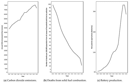
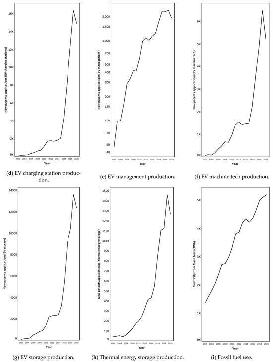
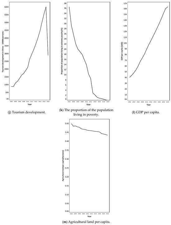
Figure 2.
Trends in China’s carbon emissions and drivers (2002–2020).
Figure 3 shows the relevant force orientation diagram derived from the force-directed layout algorithm, with node size reflecting the strength of correlation with annual CO2 emissions, and larger nodes indicating stronger correlations. Yellow nodes denote positive correlations, while red nodes signify negative correlations. The line segment thickness illustrates the correlation strength between nodes, with thicker segments indicating stronger correlations. The line colour represents positive or negative correlations, with yellow indicating positive and red indicating negative. Spatial distance between nodes is influenced by correlation; weaker correlations result in greater spatial distance.
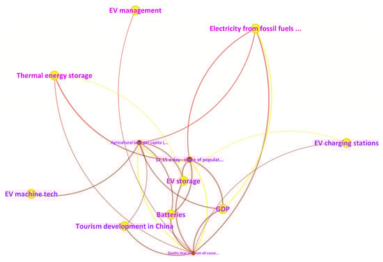
Figure 3.
Relevance Force Orientation Diagram (Red line segments indicate positive correlation, yellow line segments indicate negative correlation, red nodes indicate negative correlation with carbon emissions, and yellow nodes indicate positive correlation with carbon emissions).
The figure shows the correlation force orientation of the 12 variables of China’s annual CO2 emissions, where nine yellow nodes—EM, EFFF, TES, ECS, EMT, B, GDP (GDP per capita), TDIC, and ES—indicate a positive correlation with ACO2.
In Figure 4, the labels on the X axis (horizontal) and Y axis (vertical) represent the variables of interest, and the values in the graph represent the correlation coefficients between the variables, namely between the 12 variables of our study. Filled segments denote positive or negative correlations; red signifies positive, and blue signifies negative. The colour intensity reflects the correlation strength between variables. For correlation coefficients greater than 0, values closer to 1 denote stronger correlations, while values further away indicate weaker correlations. Conversely, for coefficients less than 0, proximity to 0 signifies weaker correlations, while proximity to −1 indicates stronger correlations between variables.
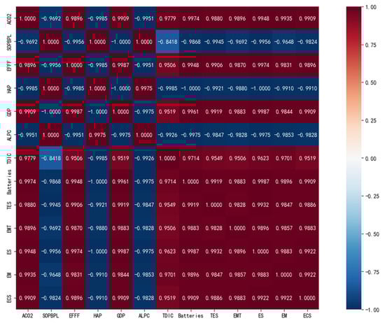
Figure 4.
Correlation heat map.
We observed a clear correlation between some variables. This includes the SOPBPL variables, which are depicted as red nodes with a larger radius in the correlation force-orientated graph. In addition, the new energy development indicators (TES, EMT, ES, EM, ECS, and Batteries) are depicted as large yellow nodes in the correlation-directed graphs, which stimulates our interest in exploring the relationship between these variables and carbon emissions.
Figure 5 depicts the normal Q–Q plot, generated through the Shapiro–Wilk test, confirming that our study’s dataset adheres to a normal distribution (p = 0.189), so we can perform a linear regression analysis of the data.
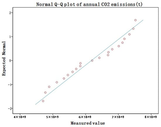
Figure 5.
Normal Q–Q plot of annual CO2 emissions.
The results of the ADF test are presented in Table 2, showing that EFFF and B are not smooth series (p > 0.05), while all the other variables are smooth series (p < 0.05).
Table 2.
The results of the ADF (augmented Dickey–Fuller) test for the model variables.
The results of the Johansen cointegration test are presented in Table 3. The test results confirmed a long-term, close relationship between the variables, and their linear combination is smooth, further substantiating the linear regression analysis results.
Table 3.
The results of the Johansen cointegration test.
The VIF test results are presented in Table 4. The analysis results reveal that the variables in this study have VIF values greater than 10, and, in some cases, even greater than 100. This suggests that there is a problem of multicollinearity between the variables.
Table 4.
Results of covariance detection between multiple variables.
Table 5 shows the expected value added of each input variable of this model from 2020 to 2030, with data adjusted on the basis of China’s 14th Five-Year Plan and Vision 2035.
Table 5.
Policy simulation.
The results of the ridge regression analysis are presented in Table 6. Based on the results of ridge regression in Table 6, we analysed the F-value and found its significance to be p < 0.01, indicating that the regression model is statistically significant. The goodness of fit, R2 = 0.98, suggests that the model accounts for most of the important influencing factors and that the fitted data points are close to the regression line, demonstrating a high degree of reliability and excellent performance.
Table 6.
The results of the ridge regression analysis.
The regression equation is as follows:
The forecasting of CO2 emissions in China based on the extended STIRPAT model can be represented as follows:
Based on Equations (4) and (5), it can be concluded that the independent variables included in the model have a significant impact on China’s annual CO2 emissions. Among these factors, the most significant impact is on agricultural land per capita, which reduces carbon emissions by 0.176% for every 1% increase. The weakest factor is the mechanical technology of electric vehicles, with carbon emissions increasing by 0.003% for every 1% of growth.
Figure 6 displays the ridge trace plot of the model. The Y axis represents the standardised coefficients of the independent variables, and the X axis indicates the value of K. The relationship between R2 and K value is shown in (b). The selection principle for the value of K is to identify the minimum value where the standardised regression coefficients of each independent variable stabilise. Upon examining Figure 6, it is evident that the standardised coefficients of each independent variable stabilise gradually as the value of K approaches 0.127.
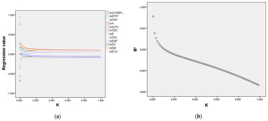
Figure 6.
The ridge traces of the model variables, the relationship between R2, and the ridge regression coefficient K, (a) denotes the relationship between the regression values of the variables and the ridge regression coefficients K, (b) denotes the relationship between the model’s goodness-of-fit, R2, and the ridge regression coefficients K.
Figure 7 displays the fitted values compared with the true values for carbon emissions. The black curve represents the true value, while the red curve represents the fitted value, and the cyan-filled area represents the difference between the fitted value and the true value. Based on Figure 8, it can be observed that the fitted curve closely approximates the true curve, with a maximum error of 3.1%, a minimum error of 0.018%, and an average error of less than 2%. This indicates that the fitted curve is highly reliable.
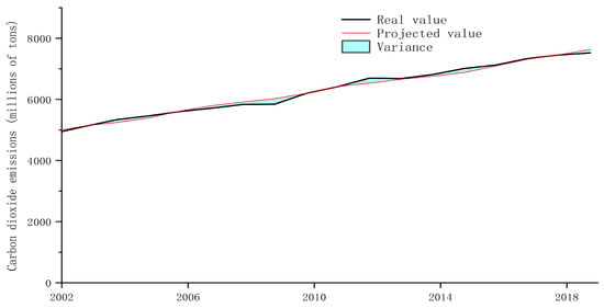
Figure 7.
Comparison of predicted and true values from ridge regression.
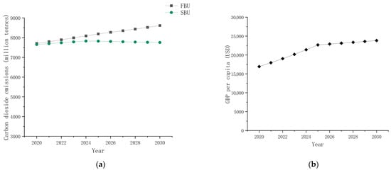
Figure 8.
Carbon dioxide emissions and GDP per capita projections for China, (a) represents the projected curve of China’s carbon emissions under the two carbon emission policies, and (b) represents the projected curve of China’s GDP per capita.
Figure 8a shows the carbon emission projections of this model for China from 2020 to 2030, showing how carbon emissions change over time, with the Green Scenario SBU reaching peak carbon emission by 2030 and the Baseline Scenario FBU not reaching it, while (b) shows the projected GDP per capita for 2020–2030.
4. Discussion
Our analysis of the various data sources reveals some critical insights into the relationship between different sectors, and their effects on carbon emissions. All our data derived from the extended STIRPAT model had an R2 fit of 0.98, indicating good reliability, and predictability in our results.
The trends seen in Figure 2, with some variables having decreasing trends and other ones having increasing trends, may be influenced by a variety of underlying factors: governments may have implemented poverty reduction and environmental protection policies that may have driven trends in the poverty headcount ratio and improved air quality; at the same time, economic growth and technological advances may have led to an increase in fossil fuel use and GDP per capita, the specific details of which are not discussed in this paper. Conversely, ACO2, TDIC, TES, EMT, ES, EM, B, and ECS displayed an increasing trend before 2019, followed by a sudden decrease after 2019, likely attributed to the novel COVID-19 pandemic, because tourism and industrial activities were restricted globally during this period [50].
From our force-directed diagram in Figure 3, we find that the spatial distances between these nodes are more compact, suggesting a closer correlation between ES, B, and G than the other variables.
Conversely, EM, EFFF, TES, and EMT are more distant, indicating lower mutual influence. EMT stands out as relatively independent and less susceptible to the influence of other variables.
Additionally, the figure shows three red nodes—ALPC, SOPBPL, and HAP—indicating a negative correlation with ACO2; these correlations may represent variables influenced by measures such as emissions reduction policies, clean energy technologies, or carbon neutrality.
From Figure 8, we find that for each 1% increase in per capita GDP, there is a corresponding increase of 0.031% in carbon emissions in the baseline scenario (FBU), showing that the long-term relationship between carbon emissions and GDP per capita does not show an inverted U-shape curve. This suggests that China’s economic growth is strongly correlated with its carbon emissions, and the results of Imen Tebourbi’s study on five developing countries in the ASEAN region, which found a strong correlation between carbon emissions and the economy using a pooled mean group estimator, which is a common drawback in developing countries globally, agree with ours [51]. Therefore, hypothesis 1 is rejected.
From Equation (5), we find that for every 1% increase in EFFF, carbon emissions increase by 0.036%, which indicates that fossil fuels have the largest positive driving effect on carbon emissions in China, thus confirming hypothesis 2. Chinese policymakers should be aware of China’s heavy reliance on fossil fuels, and promoting the green transformation of energy-consuming firms and the establishment of a mature and stable carbon emissions trading market will help to alleviate this problem. The results of our study are consistent with the results of Jiaxi’s study. Our results are consistent with the study by Jiaxi Cao in 2023, which the researchers used the standard deviation ellipse, emission kernel density, and the Terrell index to analyse the spatial and temporal characteristics and dynamic evolution of carbon dioxide emitted from fossil fuels in China from 2000 to 2019, and which also used a genetic algorithm (GA)-optimised backpropagation (BP) neural network to predict that the amount of fossil fuel-generated CO2 will continue to grow in the coming years and that fossil fuel combustion in China is a major contributor to carbon emissions [52].
Our ridge analysis also determined that for each 1% increase in electric vehicle charging stations, electric vehicle management technologies, electric vehicle energy storage technologies, electric vehicle machine technologies, thermal energy storage technologies, and battery technologies, vehicle carbon emissions will increase by 0.004%, 0.012%, 0.006%, 0.003%, 0.009%, and 0.011%, respectively. We discovered that an increase in new energy technology patents correlated with an increase in carbon emissions. Potentially in the short term, this may be due to how the development of new energy sources will require more fossil fuel consumption, and thus indirectly increase carbon emissions, an idea supported by [53], Therefore, simply expanding the new energy market may not be an effective measure to reduce carbon emissions. Instead, pursuing high-quality development of the new energy sector is a more practical approach to curbing carbon emissions. The long-term effects, however, are not clear, and would need to be explored further in future research. Thus, hypothesis 3 is rejected.
According to the FBU model shown in Figure 8, carbon emissions are projected to grow linearly, which means that China is not expected to meet its carbon emissions target by 2030. Therefore, hypothesis 4 is rejected. Our findings are consistent with Weidong Liu’s study in 2022, which developed a mathematical model to simulate different scenarios related to carbon intensity reduction through the random forest algorithm, and the results suggest that a scenario with a high percentage of fossil energy consumption may not allow China to meet its target of carbon peaking by 2030 [54].
From our results, we can determine that if the government aims to reduce ACO2 emissions without significantly impacting other variables, it could focus on suppressing EMT. Various other methods may be implemented to help China reach its goals.
4.1. Policy Recommendations
Based on the results of this study and existing research, we propose the following policy recommendations to help China achieve its 2030 carbon emissions target:
4.1.1. Pro-Poor Policy Adjustment
From Equation (5), we see that every 1% reduction in the proportion of people in extreme poverty will lead to a 0.007% increase in carbon emissions. This result is supported by Philip Wollburg’s findings, showing that pro-poor policies do not exacerbate carbon emissions [55]. However, regional differences may lead to different results, and are beyond the current scope of our study.
Therefore, we suggest that regional differences be considered and investigated more thoroughly in future research before formulating pro-poor policies to minimise the possible impact on carbon emissions.
4.1.2. Sustainable Development of Tourism and Agriculture
According to Equation (5), every 1% increase in tourism will lead to a 0.026% increase in carbon emissions, and every 1% decrease in agriculture will lead to a 0.176% increase in carbon emissions. This relationship is supported by Zhang Jiekuan’s study, which emphasises the two-way causal relationship between carbon emissions and tourism [56], and Congjia Huo’s study, confirming that increased agricultural productivity suppresses the intensity of agricultural carbon emissions [57]. In order to reduce the negative impact of tourism and agriculture on carbon emissions, we suggest the following measures:
- Formulate and implement a sustainable development plan for the tourism industry, including promoting green tourism and low-carbon modes of transport;
- Strengthen the regulation of carbon emissions from tourist attractions and hotels, and promote their adoption of clean energy and energy-saving technologies.
4.1.3. Economic Growth and Energy Use
Our results indicate a strong causal relationship between economic growth and fossil fuel utilisation with carbon emissions, correlating with Li Rongrong’s global-scale study [58]. Based on this finding, we recommend the following:
- Formulate and implement stricter energy use policies, promoting the use and development of clean energy, and establishing a mature and stable carbon emissions trading market;
- Encourage enterprises to adopt more environmentally friendly and efficient production processes and technologies to reduce energy consumption and carbon emissions.
4.1.4. Reduce Solid Fuel Air Pollution
According to Equation (5), every 1% decrease in the number of deaths caused by air pollution from solid fuels will result in a 0.026% increase in carbon emissions, a relationship that is not very well studied in the present literature. However, based on the relationship shown in our results, taking the following measures will help to reduce solid fuel air pollution:
- Promote developing and applying clean energy technologies to replace traditional solid fuel use;
- Develop and implement stricter solid fuel emission standards and regulatory measures to reduce air pollutants from solid fuel combustion.
4.1.5. High-Quality Development of the New Energy Sector
From our results, we find that the rapid development of new energy technologies exacerbates carbon emissions, a notion supported by Cang Dingbang’s findings in 2021 [53]; from that relationship, we recommend the following:
- That governments formulate comprehensive new energy policies, including support for technological innovation, guidance on industrial policies, market regulation, and international cooperation, to promote high-quality development of the new energy sector so as to effectively reduce carbon emissions from vehicles and achieve the goal of sustainable development;
- Policies for the high-quality development of the new energy sector should include promoting the construction of more electric vehicle charging stations, especially in cities and high-density-population areas;
- That the government provides financial support and tax incentives to encourage enterprises and individuals to invest in the construction of charging infrastructures, strengthen the research, development, and application of electric vehicle management technologies, encourage the research and application of more efficient electric vehicle energy storage technologies, improve the overall vehicle performance and manufacturing process of electric vehicles, and reduce energy consumption and carbon emissions;
- Investing in supporting the research and development of thermal energy storage technologies to improve energy utilisation efficiency and reduce carbon emissions, especially in applying renewable energy sources such as solar and wind energy;
- Strengthening research and innovation in battery technology to improve the energy density, cycle life, and safety of batteries and promote the development and popularisation of electric vehicles.
4.1.6. Summary of Policy Recommendations
In summary, our study provides the following policy recommendations for China to achieve its 2030 carbon emission targets:
- Adjust poverty alleviation policies to take into account regional differences and reduce the possible impacts of carbon emissions;
- Formulate and implement a sustainable development plan for tourism to reduce the negative impact of tourism on carbon emissions;
- Formulate and implement stricter energy use policies to promote the use and development of clean energy;
- Strengthen the regulation of air pollution from solid fuels and reduce air pollutants from solid fuel combustion, thereby reducing carbon emissions.
These recommendations, however, are simply derivatives of the relationships between our chosen 12 factors and China’s carbon emissions obtained from our results. Thus, confirming the effects of these policies, both short-term and long-term, are beyond the scope of our study. In future research, the problem of linear model limitations will be solved by machine learning regression models such as random forest.
5. Conclusions
China’s carbon emission targets have become more scrutinized in recent times due to rising global concerns for environmental issues, with China being one of the major contributors to carbon emissions. In analysing various factors, including those less researched, we can see if China can reach their commitment to the carbon peak by 2030, while also providing insights into the relationship between carbon emissions and the less studied factors.
Based on the extended STIRPAT model constructed in this study and the ridge regression results, we found that China’s carbon emissions are significantly affected by the proportion of people living in extreme poverty, air pollution, agricultural land, tourism development, fossil fuel power generation, and new energy sources. Correlation and regression analyses indicate that agricultural land per capita significantly impacts China’s annual carbon dioxide emissions, followed by fossil fuel power generation. This highlights the importance of government agencies balancing economic development with environmental protection. From the influence these factors have on China’s carbon emissions, as well as carbon emission projections constructed from the two scenarios created in China’s 14th Five-Year Plan and Vision 2035, we can determine that China is currently not on track to achieve its goal of achieving the carbon peak by 2030. From the results of past studies, we also provided some policy recommendations that may help China reach its goals.
Through the establishment of an analytical framework based on the extended STIRPAT model, exploring the ways to reach the peak of carbon emissions through the implementation of environmental policies by analysing the main drivers of carbon emissions in China in depth, while providing an in-depth analysis of the relationships between the less analysed drivers of carbon emissions, establishing a force-oriented network diagram data analysis framework that provides an in-depth understanding of the main drivers of carbon emissions in China, and determining the ability of China to reach its carbon emission commitments, this study fills in the gaps left by existing knowledge to the best of our knowledge.
Additionally, this study provides valuable policy recommendations and theoretical insights for policy makers and environmental experts. These policies include focusing on agricultural development, phasing out high energy-consuming industries, focusing on carbon emission reduction in parallel with poverty alleviation, establishing a sound monitoring system for the tourism industry, accelerating the green transformation of coal enterprises, and pursuing the high-quality development of the new energy sector. These recommendations provide a feasible carbon reduction pathway for achieving the commitment to peak carbon emissions by 2030.
This study contributes to further development in the theoretical understanding of the various factors that contribute to carbon emissions in China, particularly with the currently less researched factors, encouraging continued study on the effects of new energy technologies, poverty, agriculture, and tourism on carbon emissions, especially in EMT, as it seems to affect carbon emissions in a significant manner, while not currently being well researched in terms of its effects on carbon emissions to the best of our knowledge.
In future research, the problem of linear model limitations will be solved by machine learning regression models such as random forest, which will help to improve forecast reliability. Moreover, the random forest regression model does not require smooth data input, which broadens the application field of the model. Evaluating the importance of random forest features can help determine the degree of contribution of the feature variables, filter out the main driving factors of China’s carbon emissions, and finally, allow us to obtain a carbon emissions prediction model with high stability and high accuracy. By applying these nonlinear models, we will be more confident in predicting China’s carbon emissions, and be able to provide more accurate and insightful information for policymakers.
Author Contributions
Conceptualisation, S.L. and J.H.; methodology, S.L. and J.H.; software, S.L. and J.H.; validation, S.L., J.H. and S.H.; formal analysis, S.L. and J.H.; investigation, S.L., J.H. and S.H.; resources, S.L. and J.H.; data curation, S.L. and J.H.; writing—original draft preparation, S.L. and J.H.; writing—review and editing, S.L., J.H. and S.H.; visualisation, S.L. and J.H. All authors have read and agreed to the published version of the manuscript.
Funding
This research was funded by Shaoyang University Innovation Foundation for Postgraduate, grant number CX2023SY045.
Institutional Review Board Statement
Not applicable.
Informed Consent Statement
Not applicable.
Data Availability Statement
Data available in a publicly accessible repository that does not issue DOIs Publicly available datasets were analysed in this study. This data can be found here: https://github.com/stevenhua2020/atmosphere-15-00695 (accessed on 1 May 2024).
Conflicts of Interest
The authors declare no conflicts of interest.
References
- Wang, Z.; Yang, Z.; Zhang, Y.; Yin, J. Energy technology patents-CO2 emissions nexus: An empirical analysis from China. Energy Policy 2012, 42, 248–260. [Google Scholar] [CrossRef]
- China and UK Increase Commitment to a Carbon Neutral Future(acs.org). Available online: https://cen.acs.org/energy/China-UK-increase-commitment-carbon/98/i40 (accessed on 12 September 2023).
- China Not Getting Rid of Coal in Five-Year Plan as it ‘Crawls’ towards Carbon Neutrality—Carbon Brief (carbonbrief.org). Available online: https://www.carbonbrief.org/daily-brief/china-makes-no-shift-away-from-coal-in-five-year-plan-as-it-crawls-to-carbon-neutrality/ (accessed on 1 October 2023).
- The Guardian. Available online: https://www.theguardian.com.au/ (accessed on 1 October 2023).
- Lin, C.; Huang, R.J.; Ceburnis, D.; Buckley, P.; Preissler, J.; Wenger, J.; Rinaldi, M.; Facchini, M.C.; O’Dowd, C.; Ovadnevaite, J. Extreme air pollution from residential solid fuel burning. Nat. Sustain. 2018, 1, 512–517. [Google Scholar] [CrossRef]
- Hanif, I. Impact of economic growth, nonrenewable and renewable energy consumption, and urbanisation on carbon emissions in Sub-Saharan Africa. Environ. Sci. Pollut. Res. 2018, 25, 15057–15067. [Google Scholar] [CrossRef] [PubMed]
- Jiangxi Provincial Department of Science and Technology and Other Nine Departments on the Issuance of Jiangxi Provincial Science and Technology Support for Carbon Peak Carbon Neutral Implementation Programme (2022–2030). Available online: http://www.jxfc.gov.cn/fcsrmzf/zcwje5/202212/b0124786e08c49f8852061fdf298ac59.shtml (accessed on 13 September 2023).
- Jiangxi Provincial People’s Government on the Issuance of Jiangxi Province Carbon Peak Implementation Programme Notice. Available online: https://www.jiangxi.gov.cn/art/2022/7/18/art_396_4033340.html (accessed on 12 September 2023).
- Guo, Y.; Zhou, Y.; Liu, Y. Targeted poverty alleviation and its practices in rural China: A case study of Fuping county, Hebei Province. J. Rural Stud. 2022, 93, 430–440, ISSN 0743-0167. [Google Scholar] [CrossRef]
- China’s Role in Poverty Eradication (worldbank.org). Available online: https://www.worldbank.org/en/news/opinion/2016/10/17/chinas-role-in-efforts-to-eradicate-povertyTitleofSite (accessed on 1 September 2023).
- Liu, M.; Feng, X.; Wang, S.; Qiu, H. China’s poverty alleviation over the last 40 years: Successes and challenges. Aust. J. Agric. Resour. Econ. 2020, 64, 209–228. [Google Scholar] [CrossRef]
- Wan, G.; Hu, X.; Liu, W. China’s poverty reduction miracle and relative poverty: Focusing on the roles of growth and inequality. China Econ. Rev. 2021, 68, 101643. [Google Scholar] [CrossRef]
- Global Multidimensional Poverty Index (MPI) 2021|Human Development Report (undp.org). Available online: https://hdr.undp.org/content/2021-global-multidimensional-poverty-index-mpi (accessed on 1 May 2024).
- Nabi, A.A.; Shahid, Z.A.; Mubashir, K.A.; Ali, A.; Iqbal, A.; Zaman, K. Relationship between population growth, price level, poverty incidence, and carbon emissions in a panel of 98 countries. Environ. Sci. Pollut. Res. 2020, 27, 31778–31792. [Google Scholar] [CrossRef]
- Bruckner, B.; Hubacek, K.; Shan, Y.; Zhong, H.; Feng, K. Impacts of poverty alleviation on national and global carbon emissions. Nat. Sustain. 2022, 5, 311–320. [Google Scholar] [CrossRef]
- Tian, X.L.; Bélaïd, F.; Ahmad, N. Exploring the nexus between tourism development and environmental quality: Role of Renewable energy consumption and Income. Struct. Chang. Econ. Dyn. 2021, 56, 53–63. [Google Scholar] [CrossRef]
- Dietz, T.; Rosa, E.A. Effects of population and affluence on CO2 emissions. Proc. Natl. Acad. Sci. USA 1997, 94, 175–179. [Google Scholar] [CrossRef]
- Liu, D.; Bowen, X. Can China achieve its carbon emission peaking? A scenario analysis based on STIRPAT and system dynamics model. Ecol. Indic. 2018, 93, 647–657. [Google Scholar] [CrossRef]
- Ma, M.; Yan, R.; Cai, W. An extended STIRPAT model-based methodology for evaluating the driving forces affecting carbon emissions in existing public building sector: Evidence from China in 2000–2015. Nat. Hazards 2017, 89, 741–756. [Google Scholar] [CrossRef]
- Shahbaz, M.; Loganathan, N.; Muzaffar, A.T.; Ahmed, K.; Jabran, M.A. How urbanisation affects CO2 emissions in Malaysia? The application of STIRPAT model. Renew. Sustain. Energy Rev. 2016, 57, 83–93. [Google Scholar] [CrossRef]
- Ofori, E.K.; Li, J.; Gyamfi, B.A.; Opoku-Mensah, E.; Zhang, J. Green industrial transition: Leveraging environmental innovation and environmental tax to achieve carbon neutrality. Expanding on STIRPAT model. J. Environ. Manag. 2023, 343, 118121. [Google Scholar] [CrossRef] [PubMed]
- Lohwasser, J.; Schaffer, A.; Brieden, A. The role of demographic and economic drivers on the environment in traditional and standardised STIRPAT analysis. Ecol. Econ. 2020, 178, 106811. [Google Scholar] [CrossRef]
- Yang, C.; Wang, Q.; Zhang, F. Dynamic nonlinear CO2 emission effects of urbanization routes in the eight most populous countries. PLoS ONE 2022, 17, e0267542. [Google Scholar] [CrossRef] [PubMed]
- Liu, W.; Luo, Z.; Xiao, D. Age Structure and Carbon Emission with Climate-Extended STIRPAT Model-A Cross-Country Analysis. Front. Environ. Sci. 2022, 9, 719168. [Google Scholar] [CrossRef]
- Li, K.; Lin, B.; Wang, F. The driving forces towards a low carbon economy using the STIRPAT model: Evidence from panel data analysis of China. Environ. Impact Assess. Rev. 2017, 62, 34–42. [Google Scholar] [CrossRef][Green Version]
- Drouin, H. Robust Correlation Analyses: False Positive and Power Validation Using a New Open Source Matlab Toolbox. Front. Psychol. 2022, 13, 663. [Google Scholar] [CrossRef]
- Efeizomor, R.O. A Comparative Study of Methods of Remedying Multicolinearity. Am. J. Theor. Appl. Stat. 2023, 12, 87–91. [Google Scholar] [CrossRef]
- Tukey, J.W. Exploratory Data Analysis; Addison-Wesley: Boston, MA, USA, 1977; ISBN 978-0201076165. [Google Scholar]
- Douglas, N.G.; Roy, D. Pea Prospects for Scientific Visualization as an Educational Technology. J. Learn. Sci. 1995, 4, 249–279. [Google Scholar] [CrossRef]
- Van Wijk, J.J. The Value of Visualization. In Proceedings of the VIS 05. IEEE Visualization, Minneapolis, MN, USA, 23–28 October 2005; pp. 79–86. [Google Scholar]
- Giest, S.; Mukherjee, I. Behavioral instruments in renewable energy and the role of big data: A policy perspective. Energy Policy 2018, 123, 360–366. [Google Scholar] [CrossRef]
- IRENA—International Renewable Energy Agency. Available online: https://www.irena.org/ (accessed on 15 November 2023).
- Energy Institute. Available online: https://www.energyinst.org/home (accessed on 17 November 2023).
- The World Bank. Available online: https://datacatalog.worldbank.org/search/dataset/0037712/World-Development-Indicators (accessed on 3 October 2023).
- Global Carbon Project. Available online: https://www.globalcarbonproject.org/ (accessed on 12 September 2023).
- National Bureau of Statistics of China. Available online: https://data.stats.gov.cn/ (accessed on 20 September 2023).
- Ember. Available online: https://ember-climate.org/data-catalogue/yearly-electricity-data/ (accessed on 12 October 2023).
- Food and Agriculture Organization of the United Nations. Available online: https://www.fao.org/ (accessed on 10 September 2023).
- Department of Economic Social Affairs of United Nations. Available online: https://unstats.un.org/sdgs/dataportal/database (accessed on 12 September 2023).
- De, S.; Sirisuriya, S.C.M. A Comparative Study on Web Scraping. In Proceedings of the 8th International Research Conference, KDU, Seville, Spain, 18–20 November 2015. [Google Scholar]
- Mahto, D.K.; Singh, L. A Dive into Web Scraper World. In Proceedings of the 2016 3rd International Conference on Computing for Sustainable Global Development (INDIACom), New Delhi, India, 16–18 March 2016; pp. 689–693. [Google Scholar]
- Ye, C.; Wu, C.; Zhang, J. Comparison of anomalous data rejection methods in metrology testing. Meas. Test. Technol. 2007, 34, 2. [Google Scholar] [CrossRef]
- You, Y.; Liang, D.; Wei, R.; Li, M.; Li, Y.; Wang, J.; Wang, X.; Zheng, X.; Jia, W.; Chen, T. Evaluation of metabolite-microbe correlation detection methods. Anal. Biochem. 2019, 567, 106–111, ISSN 0003-2697. [Google Scholar] [CrossRef] [PubMed]
- Zhang, W.-Y.; Wei, Z.-W.; Wang, B.-H.; Han, X.-P. Measuring mixing patterns in complex networks by Spearman rank correlation coefficient. Phys. A Stat. Mech. Its Appl. 2016, 451, 440–450, ISSN 0378-4371. [Google Scholar] [CrossRef]
- Spearman, C. The Proof and Measurement of Association between Two Things. Am. J. Psychol. 1987, 15, 72–101. [Google Scholar] [CrossRef]
- Sun, G.; Lv, H.Z.; Wang, D.Y.; Fan, X.P.; Zuo, Y.; Xiao, Y.F.; Liu, X.; Xiang, W.Q.; Guo, Z.Y. Visualisation analysis for business performance of Chinese listed companies based on Gephi. Comput. Mater. Contin. 2020, 63, 959–977. [Google Scholar]
- Adewale Alola, A. Risk to investment and renewables production in the United States: An inference for environmental sustainability. J. Clean. Prod. 2021, 312, 127652. [Google Scholar] [CrossRef]
- Sun, L.L.; Cui, H.J.; Ge, Q.S. Will China achieve its 2060 carbon neutral commitment from the provincial perspective? Adv. Clim. Chang. Res. 2022, 12, 169–178. [Google Scholar] [CrossRef]
- Li, J.; Irfan, M.; Samad, S.; Ali, B.; Zhang, Y.; Badulescu, D.; Badulescu, A. The relationship between energy consumption, CO2 emissions, economic growth, and health indicators. Int. J. Environ. Res. Public Health 2023, 20, 2325. [Google Scholar] [CrossRef]
- Sarkodie, S.A.; Owusu, P.A. Global assessment of environment, health and economic impact of the novel coronavirus (COVID-19). Environ. Dev. Sustain. 2021, 23, 5005–5015. [Google Scholar] [CrossRef] [PubMed]
- Tebourbi, I.; Thi Truc Nguyen, A.; Yuan, S.F.; Huang, C.Y. How do social and economic factors affect carbon emissions? New evidence from five ASEAN developing countries. Econ. Res. Ekon. Istraz. 2023, 36, 2120038. [Google Scholar] [CrossRef]
- Cao, J.; Zhang, J.; Chen, Y.; Fan, R.; Xu, L.; Wu, E.; Xue, Y.; Yang, J.; Chen, Y.; Yang, B.; et al. Current status, future prediction and offset potential of fossil fuel CO2 emissions in China. J. Clean. Prod. 2023, 426, 139207. [Google Scholar] [CrossRef]
- Dingbang, C.; Cang, C.; Qing, C.; Lili, S.; Caiyun, C. Does new energy consumption conducive to controllingfossil energy consumption and carbon emissions?—Evidence from China. Resour. Policy 2021, 74, 102427. [Google Scholar] [CrossRef]
- Liu, W.; Jiang, W.; Tang, Z.; Han, M. Pathways to peak carbon emissions in China by 2030: An analysis in relation to the economic growth rate. Sci. China Earth Sci. 2022, 65, 1057–1072. [Google Scholar] [CrossRef]
- Wollburg, P.; Hallegatte, S.; Mahler, D.G. Ending extreme poverty has a negligible impact on global greenhouse gas emissions. Nature 2023, 623, 982–986. [Google Scholar] [CrossRef] [PubMed]
- Zhang, J.; Zhang, Y. Tourism, economic growth, energy consumption, and CO2 emissions in China. Tour. Econ. 2021, 27, 1060–1080. [Google Scholar] [CrossRef]
- Zhu, Y.; Huo, C. The Impact of Agricultural Production Efficiency on Agricultural Carbon Emissions in China. Energies 2022, 15, 4464. [Google Scholar] [CrossRef]
- Tang, C.; Zhong, L.; Ng, P. Factors that influence the tourism industry’s carbon emissions: A tourism area life cycle model perspective. Energy Policy 2017, 109, 704–718. [Google Scholar] [CrossRef]


Disclaimer/Publisher’s Note: The statements, opinions and data contained in all publications are solely those of the individual author(s) and contributor(s) and not of MDPI and/or the editor(s). MDPI and/or the editor(s) disclaim responsibility for any injury to people or property resulting from any ideas, methods, instructions or products referred to in the content. |
© 2024 by the authors. Licensee MDPI, Basel, Switzerland. This article is an open access article distributed under the terms and conditions of the Creative Commons Attribution (CC BY) license (https://creativecommons.org/licenses/by/4.0/).