Abstract
Understanding the spatial–temporal patterns of air pollution is crucial for mitigation strategies, a task fostered nowadays by the generation of continuous concentration maps by remote sensing technologies. We applied spatial modelling to analyze such spatial–temporal patterns in Lombardy, Italy, one of the most polluted regions in Europe. We conducted monthly spatial autocorrelation (global and local) of the daily average concentrations of PM2.5, PM10, O3, NO2, SO2, and CO from 2016 to 2020, using 10 × 10 km satellite data from the Copernicus Atmosphere Monitoring Service (CAMS), aggregated on districts of approximately 100,000 population. Land-use classes were computed on identified clusters, and the significance of the differences was evaluated through the Wilcoxon rank-sum test with Bonferroni correction. The global Moran’s I autocorrelation was overall high (>0.6), indicating a strong clustering. The local autocorrelation revealed high–high clusters of PM2.5 and PM10 in the central urbanized zones in winter (January–December), and in the agrarian southern districts in summer and autumn (May–October). The temporal decomposition showed that values of PMs are particularly high in winter. Low–low clusters emerged in the northern districts for all the pollutants except O3. Seasonal peaks for O3 occurred in the summer months, with high–high clusters mostly in the hilly and mildly urban districts in the northwest. These findings elaborate the spatial patterns of air pollution concentration, providing insights for effective land-use-based pollution management strategies.
1. Introduction
Air pollution is considered one of the most relevant risks to human health worldwide. Thanks to technological advancements in the last decade, a significant increase in scientific research in the field has been witnessed [1]. However, while the pathophysiologic mechanisms of pollution on the human body have been known for a long time, studying the phenomenon at population scale is less straightforward, implying the collection and processing of large amounts of data. In this perspective, one of the main shortcomings of previous research in this field [2] is represented by the lack of accurate analyses regarding the spatial dimension of pollution distribution, such as spatial configuration characteristics, spatial heterogeneity, and spatial dependence [3], which represents a vital element in addressing air pollution [4], taking into account that the spatial patterns and clustering of air pollution are key to shedding light on the dynamics of pollutant concentration [5].
Recently, new possibilities have emerged in the field, mainly due to two driving factors as follows: the developments in satellite imagery, which have enabled the use of continuous mapping of pollution, solving many issues related to the use of ground stations [6]; and the implementation and widespread diffusion of advanced spatial techniques for data processing and modelling [7].
When investigating spatial associations, the base-ground methodology usually applied is spatial autocorrelation [3,5]; however, this analysis is known to affect the estimation of pollution effects [8], a particularly relevant aspect when addressing their impact on human health [9,10] by the exposure–response relationship and, in general, when developing environmental policies [4]. Specifically, the literature indicates that including residual spatial error terms improves the prediction of adverse health effects [9], as well as removing bias due to spatial patterns does, and is thus beneficial to the robustness of spatial correlation models [8], especially when estimating the covariate effect [11], therefore representing a critical adjustment to be made in spatial modelling. From a methodological viewpoint, the base on which spatial autocorrelation should be studied and modeled is the Local Indication of Spatial Association (LISA) approach [12]. The LISA statistic quantifies the degree of spatial autocorrelation between a geographical location and its neighboring areas, identifying “hot spots” and “cold spots”. For example, hot spots are areas with significantly high values surrounded by neighboring regions also exhibiting high values. This kind of analysis helps highlight territories where the recorded values (either high or low) are significantly unusual, revealing a spatial pattern. Different methods and metrics have been proposed to evaluate the LISA statistics [13], the main two being Getis-Ord Gi* [14] and Moran’s Index [12], both previously applied in similar studies about air pollution [15,16]. In this study, we decided to opt for Moran’s Index, which is slightly more recent and is more robust to spatial outliers. Additionally, it has superior availability in open source programming environments, thus favoring replicability of the analysis.
While published studies focus on some specific areas of the world, with China being the primary source of scientific production in the field [7], less is known about the dynamics of air pollution concentration in Europe, an example of this approach being provided for Germany [17]. In particular, the Lombardy region in Northern Italy is one of the most polluted areas of the European continent [18] and is consequently targeted as a study territory for the assessment of the health impact of air pollution [19,20,21]. Despite this, the scientific evidence about patterns and trends of air pollution concentration is still limited.
However, the mere identification of the spatial patterns of pollutants may not be informative enough to effectively drive policy decision-making. As a matter of fact, a critical role in autocorrelation of pollution levels is played by land use [15,16,17,22], widely assessed to be strongly intertwined with the spatial dynamics of air pollution [3,4,15,16,17,22,23,24,25,26,27,28,29,30,31,32,33]. In particular, the scientific literature recognizes that the main contribution to pollution is usually considered to be urbanization, either at the inter-urban level [23,24,25,26,27] or with a larger perspective [4,22,28,29]. Additionally, elevation, forest coverage, population density, and socioeconomic activities [3,30,31,32] are acknowledged as relevant factors, along with a protective function of the natural environments and a significant contribution to pollution concentration from agricultural areas [33]. Accordingly, the analysis of the spatial distribution of air pollution should never neglect the role of land use, at the risk of mistakenly interpreting global dynamics on a local level. Compared to the current studies on this topic, our aim was to go beyond the identification of an existing correlation between land use and clusters of air pollution concentration, as well as include a quantitative assessment and an evaluation of its statistical significance.
Therefore, the primary aim of this study was to analyze the spatial autocorrelation of air pollution concentration across the territory of Lombardy region, by computing the global and local Moran’s I across different districts. Such analysis addresses one critical research question: Are there clearly identifiable spatial and temporal patterns in air pollution in the target territory, and do they change for different pollutants? Additionally, a secondary question arises: Are there significant differences in terms of land use among areas showing specific pollution patterns? To investigate this aspect, we aimed at performing secondary post hoc analysis considering the land-use subdivision in clusters identified by spatial autocorrelation in order to assess their possible differences and their statistical significance.
2. Materials and Methods
2.1. Materials
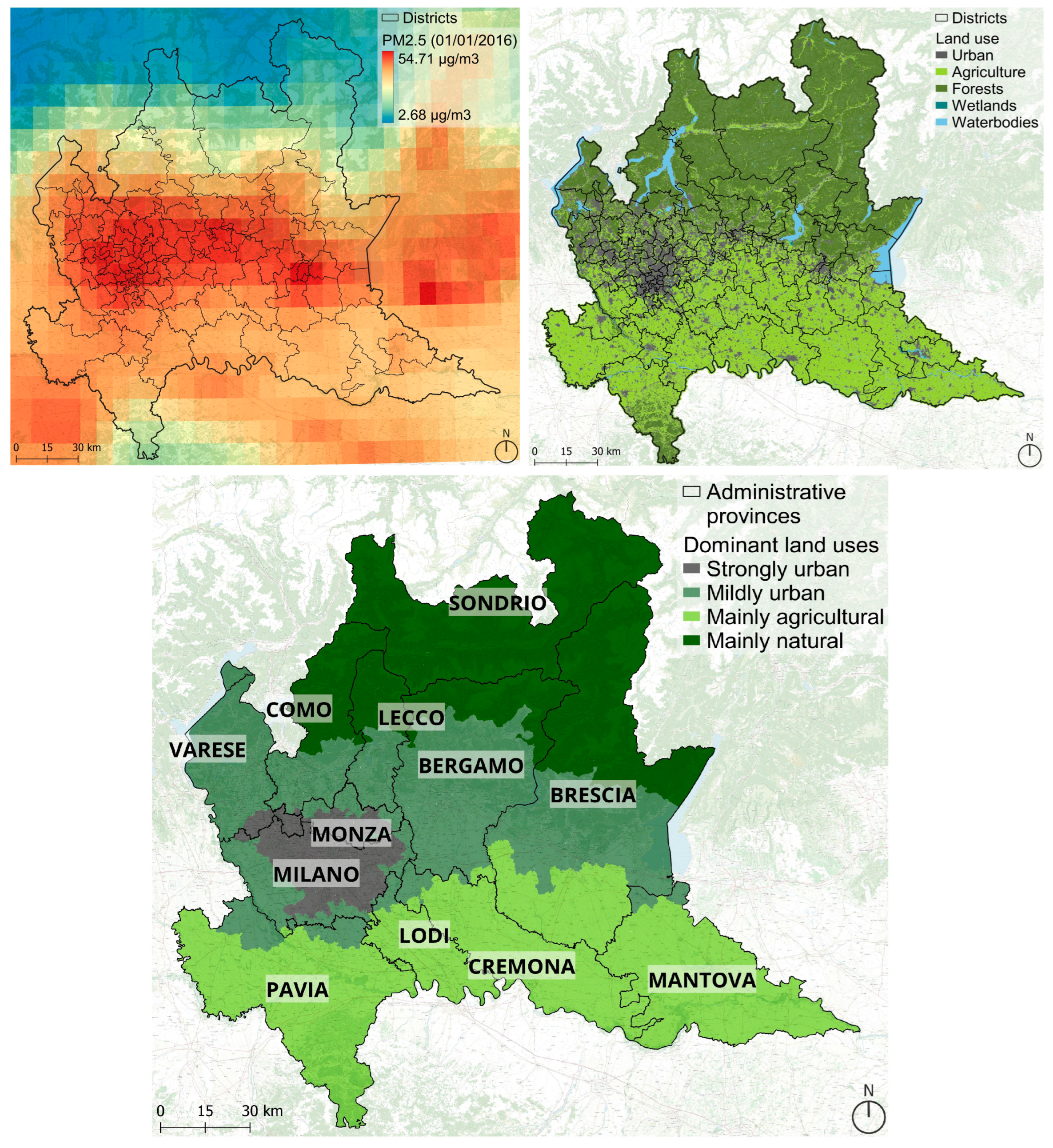
Target territory: The analysis was focused on the Lombardy region, Italy, a territory with an overall surface area of 23,844 km2, where slightly more than 10 M people currently live. Such a territory is characterized by a strong land-use diversity, encompassing densely urbanized areas (around the capital city of Milan, whose metropolitan area accounts for more than 30% of the total population, with 3.25 M inhabitants), a vast plain mainly covered by agricultural fields, lakes, and a northern (mainly natural) area, with mountains of up to 4000 m in height. Maps of the target territory with administrative boundaries and land use representation can be found in Figure 1.
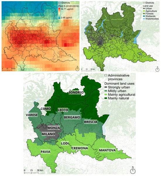
Figure 1.
Mapping of the analyzed territory of the Lombardy region, in Northern Italy, with a heatmap representation of a sample of PM2.5 concentration and the superimposed boundaries of territorial districts of approximately 100,000 residents (upper left panel), together with the land-use distribution across the territory (upper right panel), and administrative provinces with a qualitative indication of the main land-use class characterizing the territory of each district (lower panel).
Delineation of districts: The generation of pollution is strictly related to human activities, thus this gives rise to a consistent risk of detecting spurious correlations and collinearity issues. To adjust for this, the applied strategy was to consider custom territorial districts, created by aggregating neighboring municipalities, whose resident population is as uniform as possible. Targeting a total population of 100,000 residents, the resulting districts are 96 (see Figure 1). This approach was previously validated, showing a consistent robustness when studying air pollution and its effects [34].
Air quality: The hourly air quality data of PM2.5, PM10, NO2, O3, SO2 and CO from 1 January 2016 (first date of validated sanitary data availability) to 31 December 2020 (most recent available pollution data) were extracted from the CAMS (Copernicus Atmosphere Monitoring Service) European air quality re-analysis dataset, available with a spatial resolution of approximately 10 km × 10 km [35]. The data were resampled in time to result in a daily average and spatially aggregated at the scale of districts
Land use: The latest available land-use data from project DUSAF 7.0 (Destinazione d’Uso dei Suoli Agricoli e Forestali [36]) were used; they were structured into five general categories, namely anthropized areas (level 1), agricultural areas (level 2), wooded areas and semi-natural environments (level 3), water bodies (level 4), and wetlands (level 5), then further subdivided into four more levels of sub-classes. Due to the marginal presence of wetlands in the region, only the first four categories were considered, redefined into following custom classes: (I) urbanized area (level 1.1 in the original data), (II) industrial and transport facilities (level 1.2 in the original data), (III) agricultural terrains (level 2 in the original data), and (IV) natural areas (level 3 in the original data). Please note that further information about the classification system can be found in the metadata of the original database [36].
Data processing and graphical representations were handled with Python programming language (v3.10), while maps were developed in QGIS (v3.28).
2.2. Time-Series Analysis
The daily air quality data from 2016 to 2020 were decomposed using a seasonal trend decomposition method that applies a combination of local regression (LOESS smoother) [37] to extract the trend, the seasonal and remaining components of the temporal data. The monthly peaks and valleys along with the overall trend were compared with the subsequent outcomes of global and local autocorrelation of the pollutants.
2.3. Global Autocorrelation
Spatial autocorrelation helps in the understanding of the correlation between a single variable at a location and its values in a relatively close or adjacent location in a two-dimensional space. These neighboring spatial units are defined based on a n × n binary geographic connectivity/weight matrix [38]. As the territorial units in this study were defined based on irregular administrative boundaries, contiguity-based spatial weights, defined as queen criterion, were considered suitable as a neighbor structure. The queen criterion selected a maximum of eight adjoining neighbors to account for the spatial weights, W, wherein:
The spatial weights of the individual units, , are non-zero (1 in this case) when i and j are neighbors, and zero otherwise. Similarly, for self-neighbor relation where , and therefore, is excluded [39].
Following the development of the connectivity matrix and spatial weights, the global Moran’s I is calculated to effectively measure the extent of spatial randomness of the considered variable. For improved robustness of the analysis, and in light of the temporal consistency in data, spatial analyses were performed on the whole aggregated analysis period (1 January 2016 to 31 December 2020). The Moran’s I is the cross-product between the observed variable and its spatial lag , weighted based on its spatial weight in the matrix:
wherein for an observation in the spatial unit i and its neighbor , , where is the mean of variable , and is the sum of all the spatial weights and is the number of observations. However, in the case of row-standardized weights, becomes equal to the number of observations.
Moran’s I is based on the null hypothesis of spatial randomness, where the highest value of 1 corresponds to a completely positive autocorrelation, implying that high values would tend to be located near high values and vice versa. In contrast, the lowest value of −1 implies negative autocorrelation, wherein high and low values are not clustered together and are instead spatially dispersed.
2.4. Local Moran’s I Autocorrelation
As global Moran’s I autocorrelation provides only a measure of the overall spatial pattern of the observed variable, the location of the High–High and Low–Low clusters cannot be identified with it. Therefore, the local indicator of spatial association (LISA) principle, that denotes the proportional relationship between the sum of the local statistics and a corresponding global statistic, was adopted [12]. Based on the LISA principle, local Moran statistics applies the same logic as global Moran’s I but on the individual spatial unit, and estimates the statistical significance of the pattern of spatial association at location i. For such a reason, the sum of the local Moran statistics is proportional to the global Moran’s I of the variable [12].
In local Moran statistics, significance based on the assumption of standard normal distribution is often not met; thus, a more robust approach of conditional permutation is adopted, wherein the statistic is computed for randomly reshuffled datasets. The reference distribution is called, in this case, pseudo p-value, and it is useful for the classification of significant High–High and Low–Low spatial clusters. Month-wise global and local Moran’s autocorrelation of all the pollutants from 2016 to 2020 were analyzed using ESDA, an open-source python library [40], and aggregated at the scale of the districts.
2.5. Differences in Land Use
In order to investigate possible differences in the land use for the identified clusters, a novel approach was proposed in which districts were categorized as High–High or Low–Low areas if such a classification, based on local Moran’s I, resulted in significant values (p-value < 0.05) within at least 90% of the inspected timeframes (months), or were categorized otherwise as non-clustered. This selection was repeated (with consequently different results) for each considered pollutant.
Subsequently, the whole territory was divided into unit areas constituted by hexagonal cells with a diameter of 1 km. For each cell, the percentage of territory covered by (I) urban land, (II) areas dedicated to industrial activity or transport, (III) agricultural land, or (IV) natural territory was computed. The land-use characterization of each cluster of districts (High–High, Low–Low, or non-clustered) was computed as the distribution of land-use percentages across the unit area cells belonging to the corresponding districts in the different clusters.
2.6. Statistical Analysis
To evaluate for possible differences, the distributions of land-use composition in the High–High and Low–Low clusters (separately) were compared to that of the non-clustered territory. The normality of the distributions was assessed through the Shapiro–Wilk normality test, indicating if the values were to be represented as mean ± standard deviation or median (first to third quartile). In case both distributions resulted as normal, the unpaired t-test was performed to assess the statistical significance of the difference, while in other cases (at least one non-normal distribution), the Mann–Whitney U-test was implemented for the same purpose. As the total number of groups was three, the Bonferroni correction was applied to assess significance.
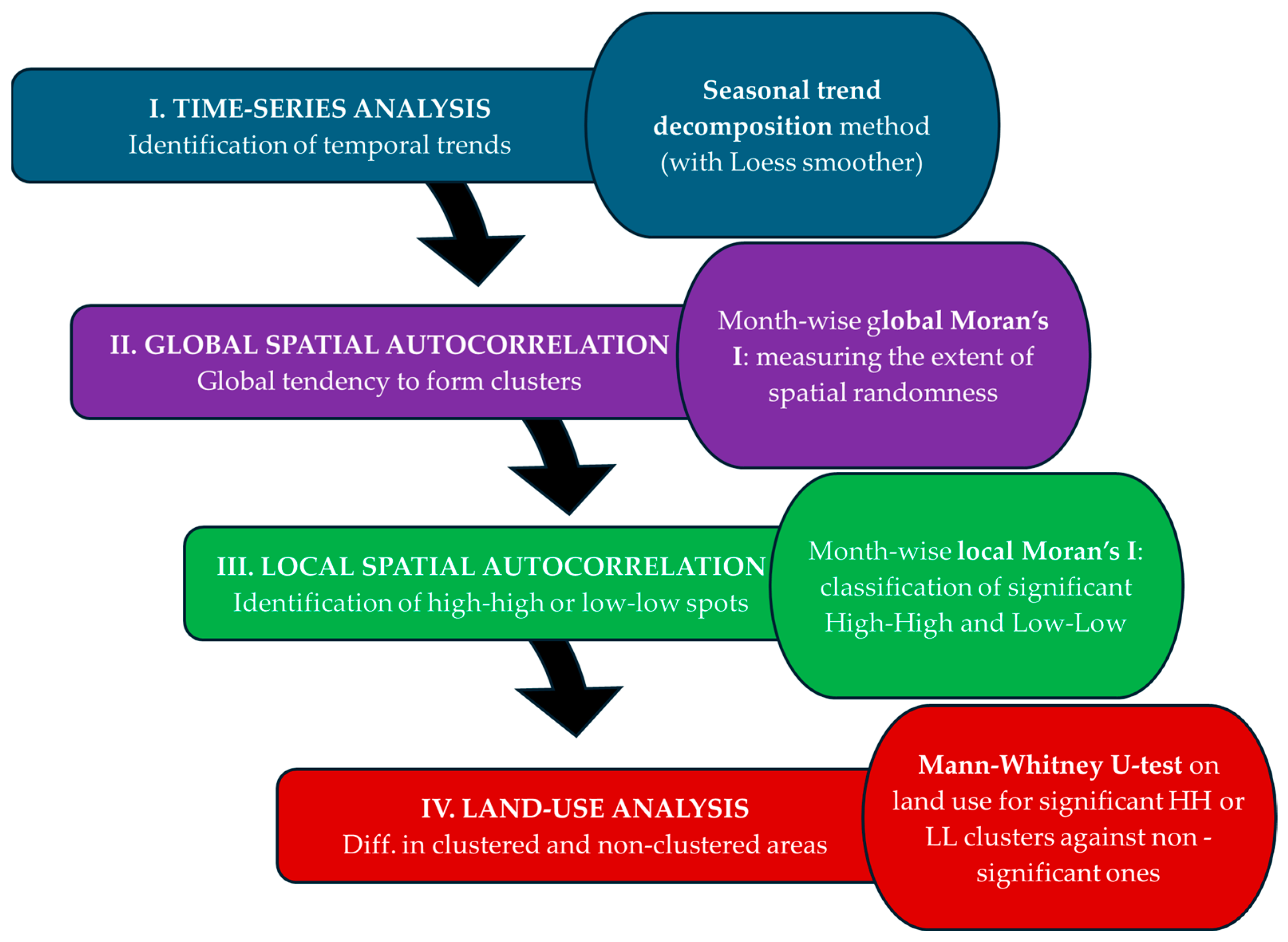
A technical roadmap of the whole analysis framework is reported in Figure 2.
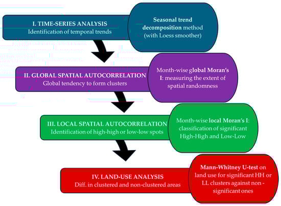
Figure 2.
Technical roadmap of the methodologies applied to infer information about the temporal and spatial patterns of air pollution concentration in the territory of the Lombardy region, in Northern Italy, and about the impact of land use into spatial clustering.
3. Results
3.1. Time-Series Analysis
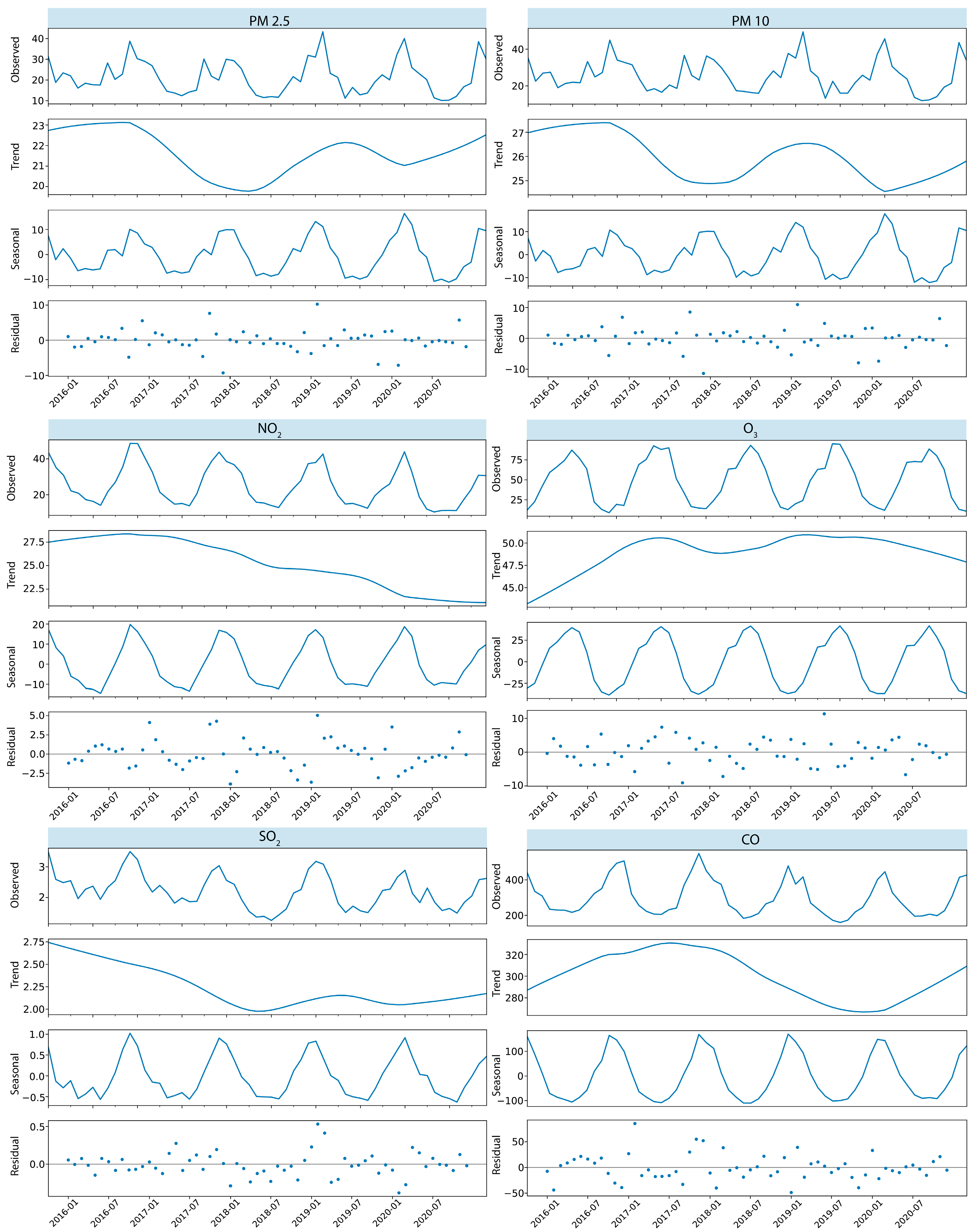
Out of the six pollutants studied, PM2.5, PM10, NO2 and O3 were found to exceed the WHO daily permissible levels. Descriptive statistics of air pollution levels from 2016 to 2020 and the days exceeding the WHO sanitary guidelines [41] are reported in Table 1. In particular, PM2.5 (21.4 µg m−3 per day) and NO2 (25.05 µg m−3 per day) surpassed such levels in 60% and 40% of the days in the studied period, respectively. All the pollutants demonstrated a seasonal pattern, with a peak localized during specific months of the year. PM2.5 and PM10 concentrations from 2016 to 2020 revealed almost parallel trends, with a major peak in January and a valley during the summer months (May–August). Apart from the seasonal pattern, the trend showed a dip in 2017 and again in early 2020, coinciding with the first COVID-19 lockdown in the region. On the other hand, NO2 underwent a steady decline since mid-2016, with a seasonal peak observed in the winter months (November–February) and a valley during summer. Winter peaks were also recorded for SO2 and CO, but these pollutants were found to be well under the daily WHO permissible limits throughout the year. On the contrary, O3 was the only pollutant with peaks during summer months, with a steady increase until 2017 and a subsequent plateau until 2020. A graphical representation of the time-series analysis is reported in Figure 3.

Table 1.
Descriptive statistics of air pollution levels from 2016 to 2020 and the days exceeding the WHO guidelines for the respective pollutant in the territory of the Lombardy region, Italy, based on Copernicus’ CAMS reanalysis data.
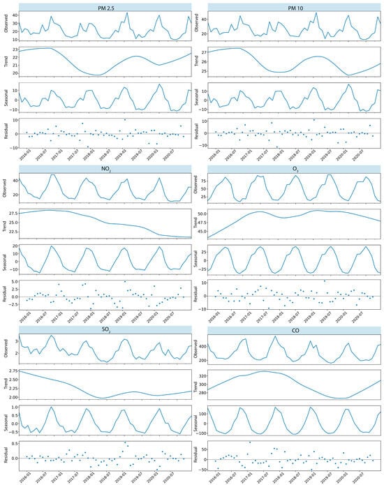
Figure 3.
Decomposition of the pollutant concentration values (µg/m3) (through trend and seasonal decomposition method—lines—based on LOESS smoother), along with the resulting residuals (dots) left after fitting the model relevant to the daily air quality data from 2016 to 2020 (as reported by Copernicus CAMS reanalysis data) for the territory of the Lombardy region, Italy.
3.2. Global Autocorrelation
The global Moran’s I, indicating the extent of spatial randomness in the pollution concentration among the districts, produced results varying by pollutant and month. The analysis demonstrated an overall high level of clustering (as reported in Figure 4), with all the months achieving values over 0.60 and soaring as high as 0.91 (recorded for CO, in April 2016 and May 2020). For NO2 and SO2, the autocorrelation was higher and more consistent in different time frames. The clustering patterns for PM2.5, PM10, and O3 showed different results and did not indicate any periodicity by month during the study period. This strong clustering pattern in the pollutants further warrants an investigation of its detailed location, which can be determined using local spatial autocorrelation.
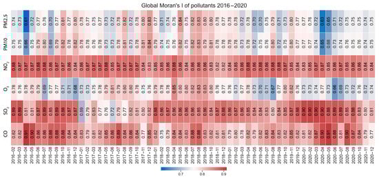
Figure 4.
Values of global Moran’s I to measure the spatial autocorrelation for different air pollutants, month by month from 2016 to 2020, on the territory of the Lombardy region, Italy. Air pollution data were derived from the Copernicus CAMS reanalysis dataset.
3.3. Local Autocorrelation
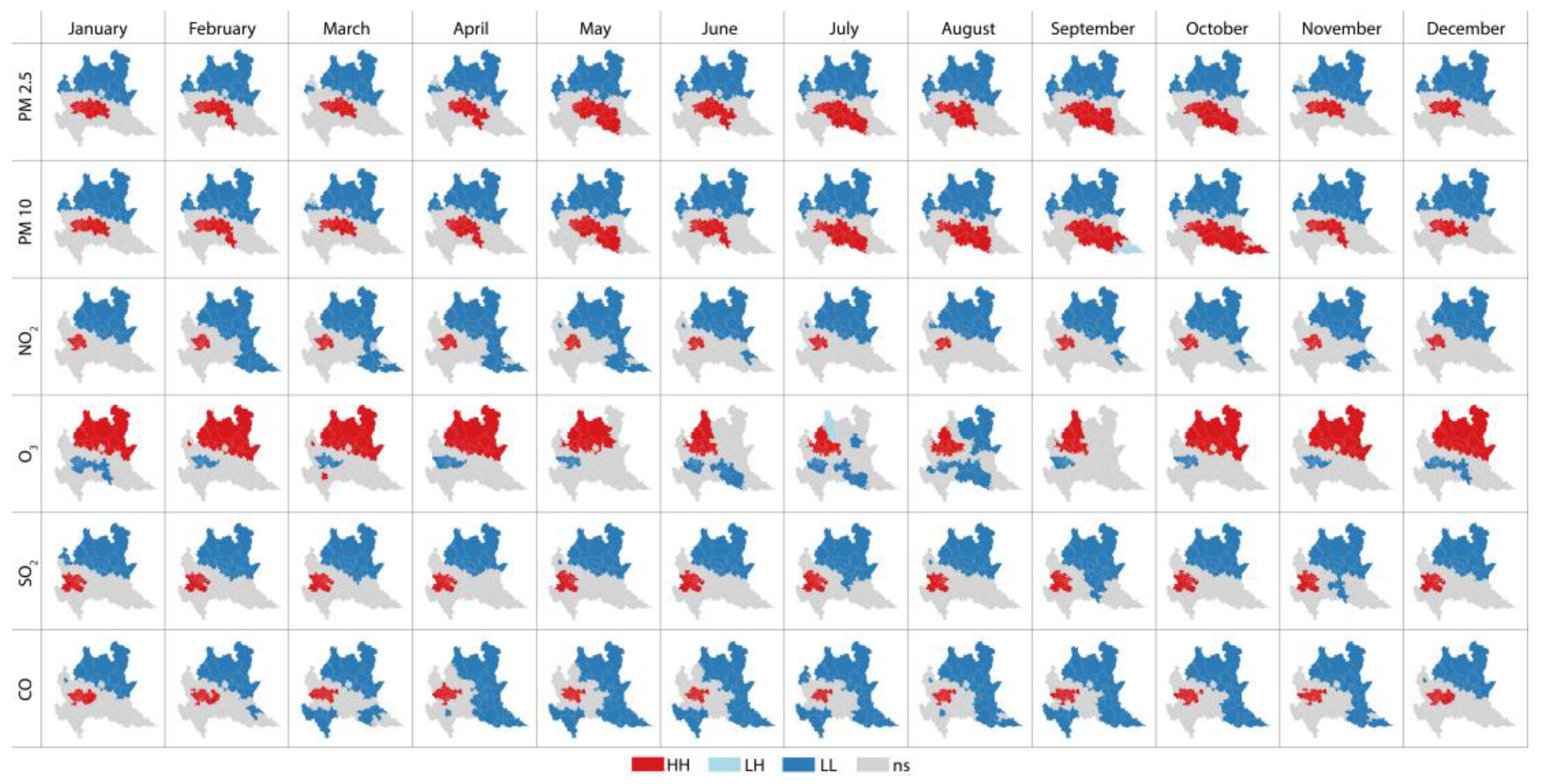
The distribution of patterns in the monthly average concentration of pollutants from 2016 to 2020 was assessed by computing local Moran’s I on the 96 territorial units with the approximately uniform population of 100,000 residents, with the complete results reported in Figure 5. As suggested by the high and positive values of global autocorrelation, results revealed a significant clustering pattern for all the pollutants. A clear north–south division emerged for PM2.5, PM10, NO2, SO2, and CO, with High–High clusters in the south, especially around the metropolitan area of Milan (most densely inhabited territory) and the city of Cremona in the southeast. During the peak winter months, from November to February, a single significant High–High cluster was concentrated within the city of Milan and its eastern peripheries, up to Cremona, whereas during the rest of the year the High–High cluster spread further in the south and southeast, especially for PM10. The Low–Low clusters for particulate matter covered the upper half of the region, characterized primarily by natural and semi-natural land cover.
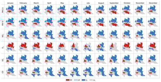
Figure 5.
Local Moran’s I computed on 96 districts with the approximately uniform population of 100,000 residents across the territory of the Lombardy region, Italy, for different air pollutants (concentration values reported by Copernicus CAMS reanalysis data). Red and dark blue areas correspond to High–High and Low–Low clusters, respectively, while the remaining areas in grey resulted as not significant for clustering purposes.
With regards to NO2, it remained concentrated within the jurisdiction of the metropolitan Milan area throughout the year, while the northern and eastern districts fell under the Low–Low cluster (and the rest of the region remained not significant in terms of clustering). This pattern could also be noticed for SO2 and CO, where, regardless of their overall low concentrations, the High–High significant cluster was larger than that of NO2 and was found within and in the adjacent districts of the metropolitan city of Milan.
Lastly, O3, which peaks during the summer months, has its significant High–High clusters in the northern districts. However, during the peak months of June–September, the cluster shrank towards the northwest in the lakeside and urban districts of Lecco, Como, and Bergamo. The Low–Low clusters with significant Moran statistics were more fragmented throughout the year and mainly located on the southern part of the region around Milan, except for the month of August, where the Northern Alpine districts of Bormio and Sondrio were also included.
3.4. Land-Use Analysis
The land-use composition was computed in the High–High cluster (HH), Low–Low cluster (LL), and non-clustered areas (Nc) separately for each pollutant according to local Moran’s I. The HH and LL clusters’ compositions were respectively compared to that of the Nc districts. As all resultant distributions did not follow a normal distribution (as assessed through Shapiro–Wilk normality test), the Mann–Whitney U-test (with Bonferroni correction) was applied to assess the significance of the differences. Complete results are reported in Table 2.
Table 2.
Distribution of land-use classes for the territory of the Lombardy region, Italy, comparing areas where different air pollutants that showed local High–High clusters, Low–Low clusters, or no clustering tendency, according to local Moran’s I. The number N of unit areas (hexagonal cells with 1 km diameter) composing each category is reported separately for each pollutant. Since all distributions resulted as non-normal, values are reported as median [1st quartile–3rd quartile]. To assess the significance of the identified differences, p-values resulting from the Mann–Whitney U-test (with Bonferroni correction) were reported.
With the only exception of urban areas percentage for PM2.5 in the HH cluster, the differences were significant (with p-value < 0.01) in all the cases. For all pollutants, excluding O3, the LL clusters showed an extremely evident larger amount of natural area (refer to Figure 1, lower panel) compared to the Nc districts, whereas an inverse relationship was observed for O3, for which a higher share of natural area characterized the HH cluster. For CO, the HH cluster was evidently composed of a larger amount of built-up area (urban, industrial, or devoted to transport facilities, again referred to in Figure 1), with a similar yet less evident distribution characterizing HH cluster for SO2, and also for NO2, for which it was furthermore possible to identify a much more consistent difference in the industrial and transport areas. Considering particulate matters (either 2.5 or 10), a significant difference emerged for industrial/transport territory, but the most considerable gap was that of agricultural areas, which were more diffused in HH clusters as compared to Nc districts.
4. Discussion
Copernicus’ CAMS re-analysis data for the period 2016–2020 were used to study the distribution of air pollution concentration on the territory of the Lombardy region, Italy, thus overcoming the limitations related to the use of a sparse system of ground stations. Temporal trends emerging from time-series analysis confirmed well-established knowledge, showing peaks of the pollutants in winter [21,42,43], except for O3, which instead reached its maximum in summer, showing a reversed dynamic that is confirmed in the literature [16]. As a primary aim of this study, the spatial trends and patterns of the concentration were inspected through spatial autocorrelation, which showed globally a strong tendency to cluster, resulting in global Moran’s I always above 0.6, reaching a maximum of 0.91. This result indicates that a strong mutual influence of the adjacent areas had occurred, confirming what similar studies have reported on different territories [2,4,16,22,44], a factor often mistakenly ignored in previous research [22]. From this evidence, it is possible to state that, regardless of the analyzed territory, clear spatial and temporal patterns in air pollution could be identified, once again in accordance with similar studies [16].
To better investigate and characterize spatial interactions, a local spatial autocorrelation analysis was also performed, computing local Moran’s I. Again with the exception of O3, an overall common trend could be observed for all other pollutants, with a High–High cluster encompassing the most urbanized area, and a Low–Low cluster covering the natural northern part of the territory, once again showing coherence with similar studies conducted on other territories [2,3,16,17,44,45]. The exact opposite behavior was observed for O3, also in agreement with previous studies [16], that represented the exception to what can be considered, in first approximation, the dynamics valid for all air pollutants.
Furthermore, in an attempt to overcome the established knowledge and deepen the understanding of spatial dynamics in air pollution concentration, after the identification of clusters through local Moran’s I, an additional analysis was implemented to take into account their differences in land use to better characterize the impact of this factor. Some additional details emerged, with almost all differences being statistically significant, allowing us to state that the secondary research question (whether there are significant differences in terms of land use among areas showing specific pollution patterns) has an affirmative answer. In particular, the most significant results were relevant to particulate matters. Despite the fact that the HH cluster included the most urbanized area, the differences in terms of % of the urban area in that HH cluster are comparable to those of the Nc districts, at the point that, for PM2.5, the difference was not significant (PM10: 3.0 [1.0–14.5]% in HH against 3.0 [0.7–11.1]% in Nc, p-value < 0.01; PM2.5: 2.8 [1.0–12.3]% in HH against 3.0 [0.7–11.1]% in Nc, p-value 0.03). On the contrary, a significant difference emerged for areas devoted to industrial activity or transports (PM10: 7.4 [2.9–21.7]% in HH, against 3.6 [0.3–12.0]% in Nc, p-value < 0.01; PM2.5: 7.3 [2.9–18.0]% in HH against 3.5 [0.3–11.9]% in Nc, p-value < 0.01) and even more consistently for the amount of agricultural area (PM10: 80.2 [51.7–91.4]% in HH against 73.3 [29.3–91.1]% in Nc, p-value < 0.01; PM2.5: 80.7 [58.3–91.4]% in HH against 73.1 [28.6–91.1]% in Nc, p-value < 0.01), as can also be observed from Figure 5, where the extension of the HH cluster towards the southeastern agricultural area of the region was evident. These findings indicate that the mutual influence on air pollution concentration of the neighboring urban areas is mainly correlated to these activities (i.e., mainly agriculture, but also transport and industry), rather than urbanization itself. Such a result, despite not being widely present in the literature, is fully coherent with a previous analysis conducted on the same territory with the aid of GeoAI [33]. Similarly, additional insightful considerations could be drawn for other pollutants. For instance, regarding NO2, the HH cluster showed a higher percentage of urban area compared to the Nc districts (16.4 [3.6–38.5]% in HH against 3.0 [0.7–10.6]% in Nc, p-value < 0.01), but the most evident difference stands in the share of areas devoted to industrial activity or transport (33.7 [12.0–52.9]% in HH against 3.8 [0.5–11.4]% in Nc, p-value < 0.01), which is coherent with the well-established knowledge that NO2 is mainly generated by traditionally fueled (combustion engines) transport vehicles [17]. Based on these observations, it is possible to conclude that the role of land use, widely discussed in the literature [3,4,15,16,17,22,23,24,25,26,27,28,29,30,31,32,33], is statistically significant. Moreover, further details on the separate impacts of different emission sources into the spatial clustering of pollution concentration could be effectively inferred with the proposed approach.
From the viewpoint of policymakers, two main results should be taken into account. First, local phenomena have significant relevance, as demonstrated by the significance of the differences in land use of the concentration spatial clusters; as a consequence, prevention and mitigation strategies developed by large-scale assessments are at risk of being poorly effective. Secondarily, at the same time, the existence of consistent spatial and temporal clusters implies that policies implemented at a local level could be ineffective, as already suggested by previous studies [2,22,44]. Therefore, the challenge to achieve better future mitigation results will be to implement policies on a large scale, while tailoring the specific interventions to a small local perspective.
The proposed study set-up presented some limitations. First of all, the use of satellite imagery, which allowed us to overcome the most relevant issues related to the use of ground-stations’ data, still has two important drawbacks as follows: I—Spatial resolution: CAMS re-analysis grid has a 10 × 10 km cell dimension, which is therefore, by some means, too coarse to correctly intercept strongly local phenomena (especially considering its crossing with a territorial subdivision based on administrative boundaries); II—Measurement quality: although CAMS data are recognized to be compliant with requirements of scientific research, the gold standard for pollution concentration in terms of accuracy is still represented by the measurement stations.
Moreover, as the specific computation of CAMS re-analysis also takes into account land use for the post processing of satellite imagery, this could possibly create a short-circuit with the performed land-use analysis, having this feature being considered both in data generation and in the following statistical analysis. However, as the land-use data were derived from a different source than CAMS, this risk should be considered acceptable for the purpose of this study. In addition, the utilized general experimental set-up, while capable of identifying spatial trends and assessing the differences among territorial clusters, is not detailed enough to precisely quantify and model the impact of land use into spatial trends.
On the basis of the obtained results, some future developments on the topic are recommended. First, a higher level of detail about land use and human activities in the territory could help shed light on the punctual local dynamics from a cause–effect relationship viewpoint, thus providing additional valuable insights for policymakers. In parallel, a higher robustness could be obtained for pollution mapping, through the combination of multiple models derived from satellite observation or ground stations. Such increased robustness could foster an improved assessment about the impact of spatial and temporal patterns of air pollution concentration into human health, both in the long- and short-term, with the consequent possibility for data-driven policymaking in terms of prevention and mitigation strategies as well as resource allocation.
5. Conclusions
The proposed study analyzed the spatial patterns of air pollution concentration in the period 2016–2020, considering six different pollutants (CO, NO2, O3, PM2.5, PM10, SO2) for the territory of the Lombardy region, in Northern Italy, recognized as one of the most polluted European areas. After a preliminary temporal explorative analysis based on time series, a spatial autocorrelation analysis was implemented through the computation of both the global and local Moran’s I. Results mainly confirmed the previous findings obtained from the analysis of different territories, showing higher pollutant concentration peaks in winter (except for O3) and a generally strong global tendency to form spatial clusters, with local dynamics highlighting that High–High clusters mainly constituted urbanized areas while Low–Low clusters encompassed the natural territories. More detailed information was derived from a post hoc assessment of the land-use characteristics for the different clusters, additionally indicating that agricultural areas have a strong influence in creating High–High clusters of particulate matters, while transportation is the main source of High–High clusters of NO2. At the same time, natural territories were confirmed as the best resource for pollution mitigation, showing a strong influence on nearby areas resulting in Low–Low pollution clusters.
Based on these results which confirm the strong spatial trends, patterns, and interactions, and in agreement with the scientific literature’s call, it is possible to reaffirm the need for a more consistent interregional perspective for policymaking in pollution management and mitigation strategies [2,22,44], despite the difficulties generated not only by administrative procedures, but also by the different economic levels, social disparities, and resource availability that may characterize the involved areas [4]. Such renewed perspective is more important now than ever, with the increasing impact of pollution on human health, especially in developed countries where this phenomenon intersects with an ageing, and therefore a more fragile population.
Author Contributions
Conceptualization, L.G., A.U.M. and E.G.C.; methodology, L.G. and A.U.M.; software, L.G. and A.U.M.; validation, L.G. and A.U.M.; formal analysis, L.G. and A.U.M.; investigation, L.G. and A.U.M.; resources, E.G.C.; data curation, L.G. and A.U.M.; writing—original draft preparation, L.G. and A.U.M.; writing—review and editing, L.G., A.U.M. and E.G.C.; visualization, L.G. and A.U.M.; supervision, E.G.C.; project administration, E.G.C.; funding acquisition, E.G.C. All authors have read and agreed to the published version of the manuscript.
Funding
L.G. is supported by the Italian project “Anthem”, funded by the National Plan for NRRP Complementary Investments (PNC, established with the decree-law 6 May 2021, n. 59, converted by law n. 101 of 2021) in a call for the funding of research initiatives for technologies and innovative trajectories in the health and care sectors (Directorial Decree n. 931 of 6 June 2022)—project n. PNC0000003—Advanced Technologies for Human-centered Medicine (project acronym: ANTHEM). AUM is attending the PhD program in Sustainable Development and Climate Change at the University School for Advanced Studies IUSS Pavia, Cycle XXXVIII, with the support of a scholarship financed by the Ministerial Decree no. 351 of 9 April 2022, based on the NRRP—funded by the European Union—NextGenerationEU—Mission 4 “Education and Research”, Component 1 “Enhancement of the offer of educational services: from nurseries to universities”—Investment 4.1 “Extension of the number of research doctorates and innovative doctorates for public administration and cultural heritage”.
Institutional Review Board Statement
Not applicable.
Informed Consent Statement
Not applicable.
Data Availability Statement
The study was conducted relying on open data only. All relevant sources are indicated in the main text.
Conflicts of Interest
The authors declare no conflicts of interest.
References
- Mehmood, K.; Bao, Y.; Saifullah Cheng, W.; Khan, M.A.; Siddique, N.; Abrar, M.M.; Soban, A.; Fahad, S.; Naidu, R. Predicting the quality of air with machine learning approaches: Current research priorities and future perspectives. J. Clean. Prod. 2022, 379, 134656. [Google Scholar] [CrossRef]
- Wang, X.; Zhou, D. Spatial agglomeration and driving factors of environmental pollution: A spatial analysis. J. Clean. Prod. 2021, 279, 123839. [Google Scholar] [CrossRef]
- Hua, W.; Junfeng, Z.; Fubao, Z.; Weiwei, Z. Analysis of spatial pattern of aerosol optical depth and affecting factors using spatial autocorrelation and spatial autoregressive model. Environ. Earth Sci. 2016, 75, 822. [Google Scholar] [CrossRef]
- Ren, L.; Matsumoto, K. Effects of socioeconomic and natural factors on air pollution in China: A spatial panel data analysis. Sci. Total Environ. 2020, 740, 140155. [Google Scholar] [CrossRef] [PubMed]
- Habibi, R.; Alesheikh, A.A.; Mohammadinia, A.; Sharif, M. An assessment of spatial pattern characterization of air pollution: A case study of CO and PM2.5 in Tehran, Iran. ISPRS Int. J. Geo-Inf. 2017, 6, 270. [Google Scholar] [CrossRef]
- Gianquintieri, L.; Oxoli, D.; Caiani, E.G.; Brovelli, M.A. Land use influence on ambient PM2.5 and ammonia concentrations: Correlation analyses in the Lombardy region, Italy. AGILE GIScience Ser. 2023, 4, 26. [Google Scholar] [CrossRef]
- Gianquintieri, L.; Oxoli, D.; Caiani, E.G.; Brovelli, M.A. State-of-art in modelling particulate matter (PM) concentration: A scoping review of aims and methods. Environ. Dev. Sustain. 2024. Published online: 2 April 2024. [Google Scholar] [CrossRef]
- Park, Y.; Kim, S.H.; Kim, S.P.; Ryu, J.; Yi, J.; Kim, J.Y.; Yoon, H.J. Spatial autocorrelation may bias the risk estimation: An application of eigenvector spatial filtering on the risk of air pollutant on asthma. Sci. Total Environ. 2022, 843, 157053. [Google Scholar] [CrossRef] [PubMed]
- Molitor, J.; Jerrett, M.; Chang, C.C.; Molitor, N.T.; Gauderman, J.; Berhane, K.; McConnell, R.; Lurmann, F.; Wu, J.; Winer, A.; et al. Assessing uncertainty in spatial exposure models for air pollution health effects assessment. Environ. Health Perspect. 2007, 115, 1147–1153. [Google Scholar] [CrossRef]
- Mahakalkar, A.U.; Gianquintieri, L.; Amici, L.; Brovelli, M.A.; Caiani, E.G. Geospatial analysis of short-term exposure to air pollution and risk of cardiovascular diseases and mortality—A systematic review. Chemosphere 2024, 353, 141495. [Google Scholar] [CrossRef]
- Lee, D.; Mitchell, R. Controlling for localised spatio-temporal autocorrelation in long-term air pollution and health studies. Stat. Methods Med. Res. 2014, 23, 488–506. [Google Scholar] [CrossRef] [PubMed]
- Anselin, L. Local Indicators of Spatial Association—LISA. Geogr. Anal. 1995, 27, 93–115. [Google Scholar] [CrossRef]
- Anselin, L. A local indicator of multivariate spatial association: Extending Geary’s c. Geogr. Anal. 2019, 51, 133–150. [Google Scholar] [CrossRef]
- Getis, A.; Ord, J.K. The analysis of spatial association by use of distance statistics. Geogr. Anal. 1992, 24, 189–206. [Google Scholar] [CrossRef]
- Zhang, Y.; Wang, S.; Feng, Z.; Song, Y. Influenza incidence and air pollution: Findings from a four-year surveillance study of prefecture-level cities in China. Front. Public Health 2022, 10, 1071229. [Google Scholar] [CrossRef] [PubMed]
- Hoffmann, L.; Gilardi, L.; Schmitz, M.T.; Erbertseder, T.; Bittner, M.; Wüst, S.; Schmid, M.; Rittweger, J. Investigating the spatiotemporal associations between meteorological conditions and air pollution in the federal state Baden-Württemberg (Germany). Sci. Rep. 2024, 14, 5997. [Google Scholar] [CrossRef] [PubMed]
- Müller, I.; Erbertseder, T.; Taubenböck, H. Tropospheric NO2: Explorative analyses of spatial variability and impact factors. Remote Sens. Environ. 2022, 270, 112839. [Google Scholar] [CrossRef]
- European Environmental Agency. Air Quality in Europe—2019 Report; Report; European Environmental Agency: Copenhagen, Denmark, 2019.
- Gilardi, L.; Khorsandi, E.; Erbertseder, T. Global Air Pollution Data for Health Risk Assessments in Lombardy, Italy. In Proceedings of the 2023 Joint Urban Remote Sensing Event (JURSE), Heraklion, Greece, 17–19 May 2023. [Google Scholar] [CrossRef]
- Gilardi, L.; Marconcini, M.; Metz-Marconcini, A.; Esch, T.; Erbertseder, T. Long-term exposure and health risk assessment from air pollution: Impact of regional scale mobility. Int. J. Health Geogr. 2023, 22, 11. [Google Scholar] [CrossRef] [PubMed]
- Otto, P.; Fusta Moro, A.; Rodeschini, J.; Shaboviq, Q.; Ignaccolo, R.; Golini, N.; Cameletti, M.; Maranzano, P.; Finazzi, F.; Fassò, A. Spatiotemporal modelling of PM2.5 concentrations in Lombardy (Italy): A comparative study. Environ. Ecol. Stat. 2024, 31, 245–272. [Google Scholar] [CrossRef]
- Yu, X.; Shen, M.; Shen, W.; Zhang, X. Effects of land urbanization on smog pollution in China: Estimation of spatial autoregressive panel data models. Land 2020, 9, 337. [Google Scholar] [CrossRef]
- Huang, X.; Cai, Y.; Li, J. Evidence of the mitigated urban particulate matter island (UPI) effect in China during 2000-2015. Sci. Total Environ. 2019, 660, 1327–1337. [Google Scholar] [CrossRef] [PubMed]
- Li, J.; Gao, Y.; Huang, X. The impact of urban agglomeration on ozone precursor conditions: A systematic investigation across global agglomerations utilizing multi-source geospatial datasets. Sci. Total Environ. 2020, 704, 135458. [Google Scholar] [CrossRef] [PubMed]
- Rodríguez, M.C.; Dupont-Courtade, L.; Oueslati, W. Air pollution and urban structure linkages: Evidence from European cities. Renew. Sustain. Energy Rev. 2016, 53, 1–9. [Google Scholar] [CrossRef]
- Song, W.; Jia, H.; Li, Z.; Tang, D.; Wang, C. Detecting urban land-use configuration effects on O2 and NO variations using geographically weighted land use regression. Atmos. Environ. 2019, 197, 166–176. [Google Scholar] [CrossRef]
- Yuan, M.; Huang, Y.; Shen, H.; Li, T. Effects of urban form on haze pollution in China: Spatial regression analysis based on PM2.5 remote sensing data. Appl. Geogr. 2018, 98, 215–223. [Google Scholar] [CrossRef]
- Li, J.; Huang, X. Impact of land-cover layout on particulate matter 2.5 in urban areas of China. Int. J. Digit. Earth 2020, 13, 474–486. [Google Scholar] [CrossRef]
- Shi, Y.; Lau, K.K.-L.; Ng, E. Incorporating wind availability into land use regression modelling of air quality in mountainous high-density urban environment. Environ. Res. 2017, 157, 17–29. [Google Scholar] [CrossRef] [PubMed]
- Liu, Y.; Wu, J.; Yu, D.; Hao, R. Understanding the patterns and drivers of air pollution on multiple time scales: The case of northern China. Environ. Manag. 2018, 61, 1048–1061. [Google Scholar] [CrossRef]
- Xu, W.; Tian, Y.; Liu, Y.; Zhao, B.; Liu, Y.; Zhang, X. Understanding the spatial-temporal patterns and influential factors on air quality index: The case of North China. Int. J. Environ. Res. Public Health 2019, 16, 2820. [Google Scholar] [CrossRef]
- Zheng, Z.; Yang, Z.; Wu, Z.; Marinello, F. Spatial variation of NO2 and its impact factors in China: An application of sentinel-5P products. Remote Sens. 2019, 11, 1939. [Google Scholar] [CrossRef]
- Gianquintieri, L.; Oxoli, D.; Caiani, E.G.; Brovelli, M.A. Implementation of a GEOAI model to assess the impact of agricultural land on the spatial distribution of PM2.5 concentration. Chemosphere 2024, 352, 141438. [Google Scholar] [CrossRef] [PubMed]
- Gianquintieri, L.; Brovelli, M.A.; Pagliosa, A.; Bonora, R.; Sechi, G.M.; Caiani, E.G. Geospatial Correlation Analysis between Air Pollution Indicators and Estimated Speed of COVID-19 Diffusion in the Lombardy Region (Italy). Int. J. Environ. Res. Public Health 2021, 18, 12154. [Google Scholar] [CrossRef] [PubMed]
- Institut national de l‘environnement industriel et des risques (Ineris); Aarhus University; Norwegian Meteorological Institute (MET Norway); Jülich Institut für Energie- und Klimaforschung (IEK); Institute of Environmental Protection—National Re-search Institute (IEP-NRI); Koninklijk Nederlands Meteorologisch Instituut (KNMI); METEO FRANCE; Nederlandse Organi-satie voor toegepast-natuurwetenschappelijk onderzoek (TNO); Swedish Meteorological and Hydrological Institute (SMHI); Finnish Meteorological Institute (FMI); et al. CAMS European air quality forecasts, ENSEMBLE data. Copernicus Atmosphere Monitoring Service (CAMS) Atmosphere Data Store (ADS). 2022. Available online: https://ads.atmosphere.copernicus.eu/cdsapp#!/dataset/cams-europe-air-quality-reanalyses?tab=overview (accessed on 10 January 2024).
- Regione Lombardia. Uso e Copertura del Suolo 2021 (Dusaf 7.0); Regione Lombardia: Milan, Italy, 2021. [Google Scholar]
- Cleveland, R.B.; Cleveland, W.S.; McRae, J.E.; Terpenning, I. STL: A Seasonal-Trend Decomposition Procedure Based on Loess (with Discussion). J. Off. Stat. 1990, 6, 3–73. [Google Scholar]
- Griffith, D.A. Spatial Autocorrelation and Spatial Filtering. In Handbook of Regional Science; Springer: Berlin/Heidelberg, Germany, 2003. [Google Scholar] [CrossRef]
- Anselin, L.; Hudak, S. Spatial econometrics in practice. Reg. Sci. Urban Econ. 1992, 22, 509–536. [Google Scholar] [CrossRef]
- Rey, S.J.; Anselin, L. PySAL: A Python Library of Spatial Analytical Methods. Rev. Reg. Stud. 2007, 37, 5–27. [Google Scholar] [CrossRef]
- WHO Air Quality Guidelines. Available online: https://www.who.int/news-room/feature-stories/detail/what-are-the-who-air-quality-guidelines (accessed on 8 May 2024).
- Bao, J.; Yang, X.; Zhao, Z.; Wang, Z.; Yu, C.; Li, X. The spatial-temporal characteristics of air pollution in China from 2001–2014. Int. J. Environ. Res. Public Health 2015, 12, 15875–15887. [Google Scholar] [CrossRef] [PubMed]
- Liu, Y.; Tian, J.; Zheng, W.; Yin, L. Spatial and temporal distribution characteristics of haze and pollution particles in China based on spatial statistics. Urban Clim. 2022, 41, 101031. [Google Scholar] [CrossRef]
- Zheng, W.; Li, X.; Yin, L.; Wang, Y. Spatiotemporal heterogeneity of urban air pollution in China based on spatial analysis. Rend. Lincei 2016, 27, 351–356. [Google Scholar] [CrossRef]
- Cheng, Z.; Li, L.; Liu, J. Identifying the spatial effects and driving factors of urban PM2.5 pollution in China. Ecol. Indic. 2017, 82, 61–75. [Google Scholar] [CrossRef]

Disclaimer/Publisher’s Note: The statements, opinions and data contained in all publications are solely those of the individual author(s) and contributor(s) and not of MDPI and/or the editor(s). MDPI and/or the editor(s) disclaim responsibility for any injury to people or property resulting from any ideas, methods, instructions or products referred to in the content. |
© 2024 by the authors. Licensee MDPI, Basel, Switzerland. This article is an open access article distributed under the terms and conditions of the Creative Commons Attribution (CC BY) license (https://creativecommons.org/licenses/by/4.0/).