Article

Study of the Atmospheric Transport of Sea-Spray Aerosols in a Coastal Zone Using a High-Resolution Model

by
Alix Limoges
1,
Jacques Piazzola
1,*,
Christophe Yohia
2,
Quentin Rodier
3,
William Bruch
4,
Elisa Canepa
5 and
Pierre Sagaut
6
1
Mediterranean Institute of Oceanography (MIO UM 110), University of Toulon, CEDEX 09, 83041 Toulon, France—University of Aix-Marseille (AMU), CEDEX 07, 13284 Marseille, France
2
OSU Institut Pytheas-SIP (UMS 3470), CNRS/INSU, University of Aix-Marseille (AMU), CEDEX 07, 13284 Marseille, France
3
CNRM (UMR 3589), 31057 Toulouse, France
4
École Centrale Nantes, CNRS, LHEEA, Nantes Université, UMR 6598, 44000 Nantes, France
5
CNR-IAS, 16149 Genova, Italy
6
CNRS, Centrale Méditerranée, Aix Marseille University, M2P2 UMR 7340, CEDEX 13, 13013 Marseille, France
*
Author to whom correspondence should be addressed.
Atmosphere 2024, 15(6), 702; https://doi.org/10.3390/atmos15060702
Submission received: 8 May 2024 / Revised: 30 May 2024 / Accepted: 6 June 2024 / Published: 12 June 2024

Abstract

:
Fine-scale models for the transport of marine aerosols are of great interest for the study of micro-climates and air quality in areas of complex topography, such as in urbanized coastal areas. To this end, the MIO laboratory implemented the Meso-NH model in its LES version over the northwest Mediterranean coastal zone using a recent sea-spray source function. Simulated meteorological parameters and aerosol concentrations are compared to experimental data acquired in the Mediterranean coastal zone in spring 2008 on board the R/V Atalante. Key findings indicate that the large eddy simulation (LES) mode closely matches with the experimental data, enabling an in-depth analysis of the numerical model ability to predict variations in aerosol concentrations. These variations are influenced by different wind directions, which lead to various fetch distances typical of coastal zones.

1. Introduction

Aerosol particles play an important role in the climate through their impact on the radiative budget [1] and cloud formation [2]. Among them, particles generated by wave breaking at the air–sea interface represent a major component of the natural aerosol [3,4,5], with a major role in the Earth radiation budget [6,7]. Sea-spray aerosols play a major role in the context of climate change [8] and also have a significant impact on air quality, particularly in coastal regions [9,10], where sea-salts dominate atmospheric deposition [11,12]. The annual global average magnitude of upward scattering of solar radiation at wavelengths 0.3 4 µ m by sea-spray particles has been estimated in various studies to range between 0.08 and 6 Wm 2 (see Lewis and Schwartz [8]). The generation of sea-spray aerosols is due to the interaction between wind and waves [13]: when the wind speed increases beyond a threshold, typically around 4 ms 1 [14,15], developing waves break to dissipate excess energy. Air is entrained in the water, and when the rising bubbles burst at the surface, aerosols are injected into the atmosphere. Near the shoreline, however, the production of sea-spray mainly relates to the bathymetric processes induced by the interaction of waves with the sea floor. As breaking waves are especially abundant in the surf zone, more sea-spray aerosols per unit area and time would be generated over this zone than at open ocean [16]. Additional aerosols are also produced over the ocean’s surface from secondary processes, due to gas-to-particle conversion of gas compounds emitted from the sea that mainly involve volatile iodine compounds and biogenic volatile organic compounds, among which are dimethylsulphide and isoprene [17].
After their ejection into the surface layer, sea-spray aerosols are transported by the atmospheric dynamics in the Marine Atmospheric Boundary Layer (MABL) and influence the climate through thermodynamic processes, such as heat and sensible fluxes, which are fundamental for their impact on precipitation (see Andreas [18]) and cyclone formation [19]. An accurate description of the spatio-temporal variation of sea-spray in the atmosphere is then of interest for a better knowledge of climatological prospects. Since the 1990s, the development of Chemical Transport Models (CTMs), which are numerical research-oriented models, has played a crucial role in enhancing our understanding of atmospheric processes. However, significant predictive uncertainties remain in numerical models for sea-spray aerosols due to biases observed in commonly used emission schemes [20,21,22]. Few studies have employed high-resolution models for the study of sea-spray dynamics in real-world conditions at regional scales. Xingkun et al. [23] used the WRF model with a horizontal resolution of 1.5 km for sea-spray modeling and Aouizerats et al. [24] focused on pollutants modeling at a 500 m resolution in urban zones. Delbeke et al. [25] explored the impact of aerosols on the life cycle of stratocumulus clouds using a large eddy simulation (LES) model. About sea-spray transport in the Mediterranean coastal area, we can cite the work of Laussac et al. [26] and Tedeschi and Piazzolla [27].
In light of the above considerations, refining the description of the spray flow requires the inclusion of parameters other than wind speed, and an improvement in the modeling of the wave field and wave breaking responsible for spray production. More particularly in coastal areas, the vicinity of the shoreline affects the development of the wave field, which in turn changes the breaking wave process [28]. Fetch, the distance over which wind blows uninterrupted over water, plays a critical role in reaching an equilibrium state of the sea with the marine atmospheric boundary layer. Fetch length, along with wind speed and duration, determines the sea state. In addition, particularly in urbanized coasts, oceanic sources of aerosols can interact with anthropogenic emissions determining an increase in aerosol loading and a typical aerosol composition in coastal areas [29,30], influencing both human health [31] and artefact conservation [32,33]. Better knowledge is then needed on the intrusion of sea-spray aerosols into the coastal urbanized areas for air quality, but also for health applications and materials maintenance. To this end, we need accurate models to be able to predict sea-spray production and transport in the MABL of coastal areas with possible complex geography. Recently, Bruch et al. [34] proposed a wave-slope dependent formulation for the sea-spray source function (S3F, heirenafter B21) based on wind tunnel measurements. This new formulation has been implemented in the Meso-NH model for validation in the Bay of Biscay [35]. Bruch et al. [35] show that the Meso-NH version equipped with the B21 source term results in an improvement of the performance of the predictions in remote oceanic regions. Meso-NH is a comprehensive model available for mesoscale atmospheric studies [36] that covers a broad range of scales, from planetary waves to near-convective scales down to turbulence. This is possible via two-way grid nesting and its versatile design as the model can be used both as a Cloud-Resolving Model (CRM) and a large eddy simulation (LES), in which most of the turbulence energy is resolved, as well as a direct numerical simulation. Additionally, Bruch et al. [35] highlight the potential impact of coastal features on the turbulent and vertical transport of aerosols within coastal environments. One of the questions is now to what extent such a Meso-NH model can be relevant for coastal areas.
The present work deals with a better knowledge of the atmospheric dynamics of sea-spray aerosols in the coastal zone in order to better understand the intrusion and the local atmospheric variations of marine aerosol concentrations in such small areas. In coastal zones, the wind field can be affected by the vicinity of the coast, resulting in the occurrence of front zones or atmospheric vortexes. Since a complex coastal geometry and topography require a very detailed description of coastal geography, our aim is to study the benefit of a higher resolution model to represent the meteorological conditions and aerosol concentrations in the vicinity of the coast. To this end, the LES configuration of the Meso-NH model version 5.6 [37] using the B21 source formulation was implemented in a French Mediterranean coastal zone. We aim to study the sensitivity and relevance of aerosol models to local changes in meteorological parameters induced by proximity to the coast. To this end, we propose a comparison between the spatio-temporal variations of the sea-spray concentrations issued from the Meso-NH LES calculations and experimental data obtained along a French Mediterranean coastal zone during an oceanic scientific cruise on board the R/V Atalante, south of the Toulon Bay. Beside the assessment of the performance of the Meso-NH model, this provided the opportunity to observe the impact of the coastal configuration on the atmospheric aerosol dynamics.

2. Material and Methods
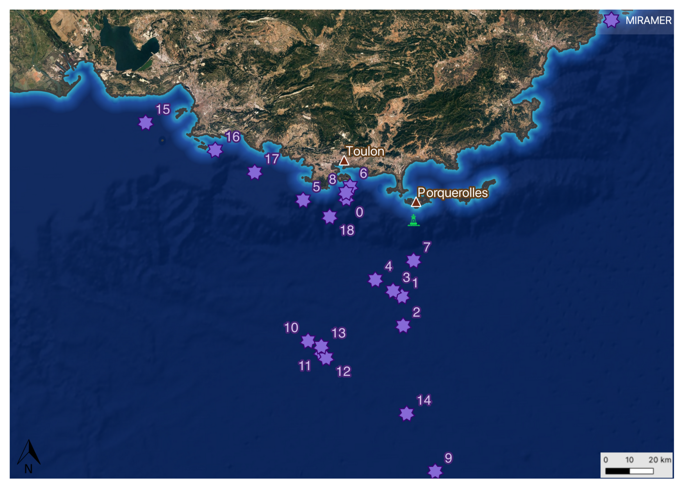
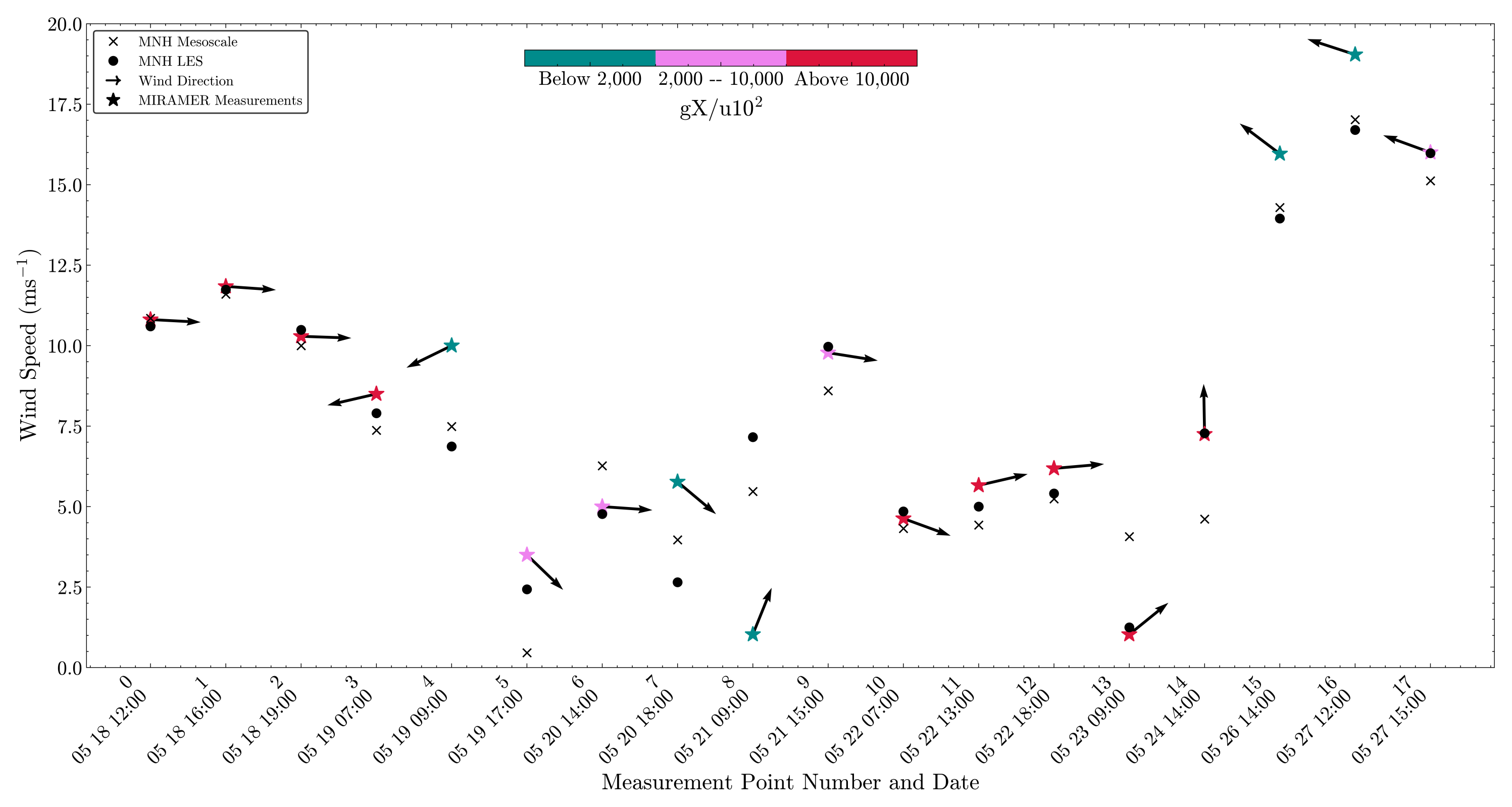
In this section, we describe the experimental setup and methodologies employed for the collection of field measurements and the implementation of the high-resolution Meso-NH model, aimed at validating the transport of sea-spray aerosols in a complex coastal zone of the northwest Mediterranean. This includes detailing the configuration of the LES mode used in the model.

2.1. Measurements

The experimental data used in this paper were collected on board the R/V Atalante during the MIRAMER experimental campaign—which took place in 2008, from May 15 to 28, in southern France (see Laussac et al. [26])—and at the extreme west point of the island of Porquerolles (Figure 1 and Figure 2). The datasets include both measurements of aerosol particle size distributions and supporting meteorological parameters. The data acquired on board the R/V Atalante during the MIRAMER campaign in 2008 provide a rare and unique set of in situ measurements at various fetches, typical of the coastal area. The study area is located south of Toulon bay, between 5.4- and 6.25-degrees east longitude and between 42.2- and 43.2-degrees north latitude (Figure 1), and it is a part of the area covered by the calculation grids used for the Meso-NH model (see Section 2.2). Figure 1 also shows where the vessel stationed for data acquisition, and the position of the meteorological buoy anchored south of Porquerolles, which is part of the CANDHIS (National Center for the Archiving of In Situ Wave Data) network and is equipped with a wave recorder for measuring sea state. This stretch of coast is exposed to air masses from the open sea, during periods when local wind directions range from west to southeast, which corresponds to infinite fetches as defined by the criterion applied for fully developed sea conditions [38], as well as to air masses originating over the European mainland, with shorter fetches [39]. In a coastal zone, fetch is one of the key parameters for sea-spray production and its atmospheric dispersion [39]. Fetch must also be considered in wind field evolution, as the coastline geography can lead to alternating land and ocean zones over which the wind travels, and hence affect wind patterns. This could probably represent a potential source of errors in the meteorological models.
On board the R/V Atalante, the probes for aerosol measurements and meteorological sensors were fixed at a height of 12 m on the mast, which was equipped with a complete MeteoFrance weather station for measuring various atmospheric variables such as relative humidity, pressure, air temperature and water temperature. Two other probes were located at the experimental station on the island of Porquerolles at a height of about 22 m above the sea surface. Aerosol data were acquired in the 0.1–95 µm size range using two co-located classical scattering spectrometers (Particle Measuring Systems, Boulder, CO, USA), the CSASP-200 and the CSASP-100HV. The data-accumulation period for the probes was 1 min, with an average stored every 4 min. It should be noted that the PMS (Particle Measuring Systems) probes use an isokinetic sampling inlet to minimize loss and to limit the effects of wind on probe flow. The transport efficiency is considered optimal for aerosol sizes below a radius of 15 µm [40], which is the range of interest for the present study. Prior to the experiments, the probes had been calibrated with latex particles of known sizes. The CSASP probes have been tested and proven reliable in numerous experiments [41,42]. The aerosol distribution associated with a given fetch and wind speed was averaged across 20 to 30 individual distributions to reduce the noise in the measurements of each distribution. Additionally, two sun photometers were installed on the island of Porquerolles and at the Sicié Cap, respectively, to complement aerosol characterization. Given the AOD values reported in the analyzed cases, we assume that the conditions during the data collection involved no significant dust interference.
The experimental campaign on board the R/V Atalante allowed to record an extensive series of data acquired at varying distances from the Mediterranean coast. Each sample available for the present study dealt with stationary conditions over durations varying from 20 to 60 min, ensuring maximum count aerosol statistics. We can define a first group of acquisitions made rather close to the south-western part of the coast (points 0, 5, 6, 8 and 15 to 18 shown in Figure 1), while a second group deals with recordings made more than one hundred kilometers south of the Toulon bay (points 1 to 4, 7 and 9 to 14, also shown in Figure 1). However, the distance between the steady location of the ship and the coastline during the acquisitions is not sufficient to characterize the influence of the coast on the measurements, as it also depends on the wind direction. For instance, the ship might be near the coast yet subject to southwest winds, resulting in larger fetches. In the coastal zone, fetch is a key parameter for sea-spray production and its atmospheric dispersion [39]. Fetch should also be considered in the context of wind field evolution, as the coastal geography, with its alternating zones of land and ocean, can significantly influence the flow of the wind. The Atalante cruise allowed meteorological and aerosol data recorded for wind sectors dealing with short to unlimited fetches. To introduce the fetch influences in our study, we used the non-dimensional fetch ξ , defined by Hsu [38], which is expressed by:
ξ = g X U 10 2
where X is the fetch (in meters), U 10 is the wind speed (in m · s 1 ) measured at 10 m height above the sea surface and g is the acceleration due to gravity ( 9.81 m · s 2 ).
The non-dimensional fetch ξ , which denotes the ratio between the distance traveled by a constant wind blowing above the sea surface and its velocity, characterizes the interaction processes between wind and waves [28]. According to Hsu [38], a value of ξ larger than 20,000 denotes fetch-limited conditions, i.e., steady wave field at the end of the fetch, whereas a non-dimensional fetch ξ smaller than 20,000 deals with unsteady conditions of the wave field, which correspond to a period of enhancement of the wave energy before an equilibrium is reached between the wave field and the wind input. At high winds, this equilibrium will be reached at a shorter fetch than for low wind speed conditions. However, for very highs winds, only a large fetch should allow exceeding 20,000. We can intuitively assume that low wind and short fetch conditions may be the most difficult conditions to describe correctly using a meteorological model. In terms of sea-spray production, we can assume that for very small ξ , the probability for the breaking occurring is very low. A specific methodology from Limoges et al. [43] is used to calculate the fetch, considering the wind trajectory above the water. This approach involves tracing the wind trajectory above the sea surface and interpreting a 30° change in wind angle as a change in wind trajectory. At this point, the streamline is considered interrupted and the fetch is calculated up to that point.

2.2. The Numerical Model

In this study, we used the Meso-NH model that is a comprehensive model available for mesoscale atmospheric studies [36] which has been jointly developed by the Laboratoire d’Aérologie (UMR 5560 UPS/CNRS) and by CNRM (UMR 3589 CNRS/Météo-France). This model has become a key player in the French research modeling community since it has been freely accessible in 2014. An alternative model used by the community is the WRF-CHEM model. Both use third and fifth order weighted essentially non-oscillatory (WENO) schemes [44]. A comparison between Meso-NH and WRF/CHEM is available in the literature [45]. Additional information and data regarding the models and simulations used in this study can be found in the Supplementary Materials.
In the present study, we use version 5.6 of the Meso-NH model. A characteristic feature of Meso-NH is that it covers a broad range of scales, from planetary waves to near-convective scales down to turbulence. However, some predictive uncertainties persist for sea-spray aerosol in numerical models, with significant biases observed for commonly used emission schemes [20,21,22].
The Meso-NH model was first used with a two-kilometer spatial resolution [37]. For the present study, the Meso-NH model operates with three two-way nesting domains at 2 km, 500 m and 200 m horizontal grid spacing respectively, as shown in Figure 3. The horizontal domain specifications are detailed in Table 1. The model grid is vertically composed of 48 layers, ranging from the mean water level to 24 km altitude. The Meso-NH model is initialized and forced at its boundaries by the ECMWF model every three hours.
Each simulation lasted 30 h with outputs every half-hour, discarding the first 6 h for model spin-up, resulting in a total of 240 simulated episodes over a period of 10 days. The days for the simulations were chosen to be specifically aligned with the MIRAMER campaign period, spanning from the 18 May 2008 to the 27 May 2008. The 17 May was not included in the simulations as the weather conditions were similar to those on 18th and was instead utilized for the model spin-up phase. More particularly for the LES version of the model, when creating the terrain grid, the smoothing of the orography was adjusted using an orography data source, i.e., SRTM (Shuttle Radar Topography Mission)_europe [46] with a 30-m resolution. In the terrain files produced by the model, we have modified the mesh to include a 50% proportion of sea, which significantly influences the wind field calculations as detailed in Section 4.
In the LES configuration, the model uses a turbulence scheme based on Redelsperger and Sommeria [47,48] and is presented in detail in Cuxart et al. [49]. Model constants are from Cheng et al. (2002) [50]. The scheme is based on a prognostic equation of the sub-grid Turbulent Kinetic Energy (TKE) and a diagnostic mixing length L m . The dissipation of the sub-grid TKE is physically induced by small-scale turbulence. Assuming that the turbulence is stationary and isotropic, dimensional arguments express the dissipation rate of TKE, ϵ , as described by the equation:
ϵ = c ϵ e 3 / 2 L ϵ
where L ϵ is the dissipation length scale, e is the kinetic energy and c ϵ is a coefficient with a value of 0.75. In this LES setting, the mixing length L m , is defined in accordance with Honnert et al. [37], in which it is proportional to the size of the grid cell, reflecting the scale of the largest energy-containing eddies within the sub-grid. The efficiency of the LES model is validated by ensuring that the resolved TKE exceeds 90% of the total kinetic energy in each LES simulation.
In the mesoscale configuration of the model, the mixing length L m is a non-local turbulent mixing length parametrisation by Bougeault and Lacarrere [51] who propose the equilibrium between TKE and buoyancy effects to determine the mixing length, where L ϵ = L m , as per the established theory in boundary-layer turbulence. This distinction between LES and mesoscale configurations underscores the different scales and processes each model is designed to capture and ensures fidelity to the respective atmospheric phenomena they are simulating.

2.3. The Emission Flux

The sea-spray source function that has been implemented in the Meso-NH model version used to perform the present study was proposed by Bruch et al. [34,35]. It combines a source function, B21, based on the wave-slope variance (denoted S 2 ) considered equal to the wave mean square slope, with the source function from Ovadnevaite et al. [52]. The latter is based on a Reynolds number, defined as R e H w = u * H s v w , where u * represents the friction velocity, H s is the significant wave height and v w is the kinematic viscosity of water.
The applicability of the wave slope variance dependent formulation by Bruch et al. [34], initially based on strong wind conditions was extended to moderate winds during the SUMOS campaign, which took place on board the R/V Atalante in 2021 [35].
The formulation by Ovadnevaite et al. [52] addresses the submicron aerosol size spectrum, whereas the wave slope-dependent function of Bruch et al. [34], is better adapted for larger particles, as indicated by the higher modal mean radius indicated in Table 2. This paper focuses on larger particles and hence the radius modes dealing with submicronic particles will not be included in our analysis. This leads to a sea-spray flux d F d r 80 for sea-spray aerosols ranging from 3 to 35 µm in size, with a distribution that is normally distributed in three modes, as follows:
d F d r 80 = i = 1 3 F i ( S 2 ) τ 1 1 σ i 2 π exp 1 2 r 80 μ i σ i 2
  • where F i is the flux for mode i:
  • S 2 is the wave-slope variance,
  • r 80 is the particle radius at 80% relative humidity,
  • σ i is the standard deviation of each of the three modes,
  • μ i is the mean radius of each of the three modes.
The parameters are presented in Table 2.
Table 2. Parameters for the Source Function B21.
i σ i μ i F i S 2
12.12.5 4.94 × 10 7 S 2 2.45
277 7.88 × 10 7 S 2 2.3
31225 1.3 × 10 7 S 2 2.39
It should be noted, however, that historically [53] and in more recent studies [54,55], authors generally consider a linear relationship between wind speed and the wave-slope variance. According to their data, Bruch et al. [35] proposed:
10 3 S 2 = 3.48 × U 10 + 3.18
where U 10 is the wind speed at 10 m.

3. Results

This section presents the results of the numerical simulations and their comparison with experimental data, focusing on wind fields and sea-spray concentrations. The key question is the applicability of the Meso-NH model using the B21 source term for sea-spray in coastal areas. Initially, this requires selecting meteorological episodes for which numerical simulations show a good agreement with the data, allowing for the assessment of the model performance for atmospheric aerosol concentrations. Therefore, the Meso-NH model was employed to compute various meteorological variables, focusing particularly on the wind field in the study area, since wind speed is a major input for aerosol model inputs. Accurate wind speed simulation presents a significant challenge for Chemical Transport Models (CTMs), especially in regions characterized by complex terrain and diverse land surface types. Consequently, coastal areas, with their variable wind conditions and intricate geometries, offer a valuable opportunity to evaluate and enhance the accuracy of meteorological model predictions. In this section, we focus on the comparison between the kilometric (2 km horizontal resolution) and LES (200 m horizontal resolution) models.

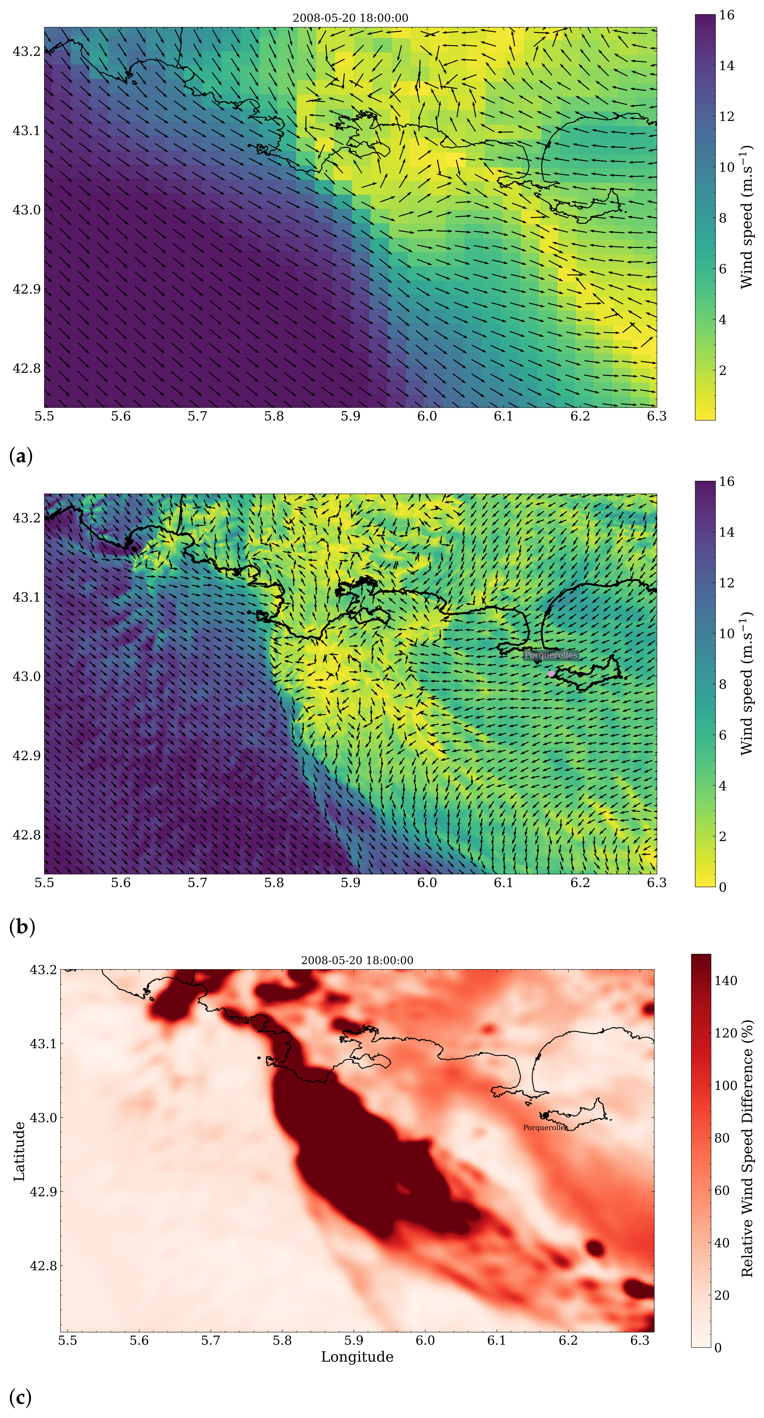
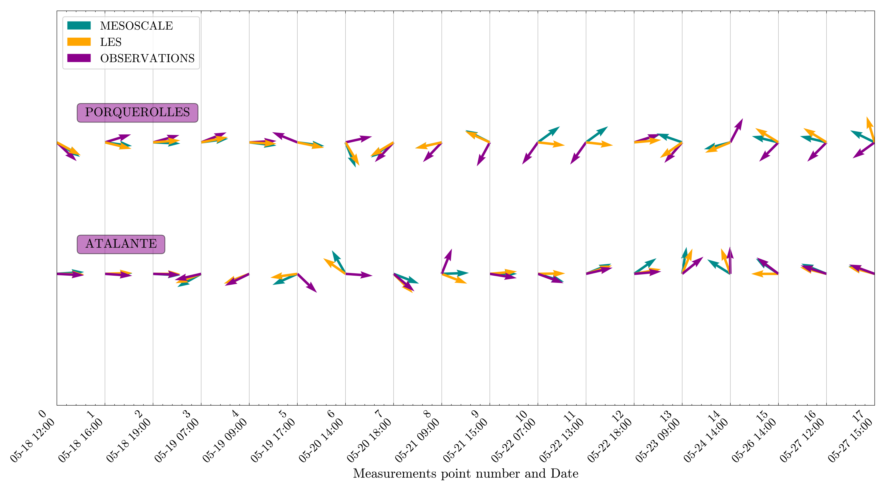
3.1. Wind Field Calculations

Figure 4, Figure 5 and Figure 6 show examples of wind fields (speed and direction) calculated for three episodes occurring during the MIRAMER campaign. Episode 1 took place on the 20 May 2008 at 6 p.m. and was characterized by a frontal zone occurrence. Episode 2 occurred on the 20 May as well, at 2 p.m. and was characterized by high wind speed of northwest direction, known as “Mistral” conditions in the study area. Episode 3 covers the period of the 19 May at 5 p.m., it was characterized by the presence of local-scale atmospheric eddies located over the sea. Each figure has three panels. Panels (a) and (b) correspond to the mesoscale (kilometric resolution) and LES calculations, respectively. The false color plot shown in Panel (c) depicts the percentage difference in wind speed between the simulation at 2 km resolution and the LES simulation with a 200 m resolution.
The first example illustrating differences between the LES and mesoscale model is shown in Figure 4, which deals with an episode of a frontal zone occurrence, i.e., winds in opposite direction on a small area, as observed south of the coastline on 20 May at 6 p.m. During the convergence of the west and easterly winds, turbulent mixing generates smaller eddies and wind patterns. Note that this meteorological phenomenon, which occurs to the south of Toulon Bay, is more detailed in the wind field provided in the LES method (Figure 4b), as shown by a diagonal line running from top left to bottom right. The distinct differences between the mesoscale and LES wind field simulations, particularly in the frontal zone, are evident when comparing Figure 4a,b. A notable observation is the spatial shift of the frontal zone, potentially accounting for the significant discrepancies in wind speed gradients between the models, as highlighted in Figure 4c. In a frontal zone, we generally observe lower wind speeds and it is conceivable that a zone of wave front also emerges.
Figure 5 presents another example from the episode on 20 May at 2 p.m., where we can note that differences between the two configurations are more pronounced near the coast. This is confirmed by Figure 5c illustrating a re-circulation of the wind near the Cape Cepet, located at the southern tip of the Saint-Mandrier-sur-Mer peninsula, leading to the generation of smaller eddies and wind patterns. The finer resolution of the grid better captures these small eddies and turbulent flows.
Figure 6 shows the wind fields calculated for the episode of 19 May at 5 p.m. In Figure 6c, we can observe an example of local-scale atmospheric eddies located over the sea; south of the Porquerolles station we can also observe a wind pattern characterized by wind in opposite directions, i.e., west and east. This also confirms that the LES resolution captures local turbulent features that the mesoscale resolution cannot resolve.
Figure 4, Figure 5 and Figure 6 show a good agreement between the data simulated using the high-resolution model and the one at kilometric resolution when the wind field is uniform, mainly in open sea. While in the cases of complex wind fields—as the frontal situation in Figure 4, the flow re-circulation near to the shoreline in Figure 5 and the complex wind pattern in Figure 6—the agreement is weaker. We can note that the difference in wind speed generally remains below 10% for a long fetch and a well-established wind in open ocean. In such conditions, the overall wind behavior appears relatively smooth and consistent, enabling both resolutions to effectively capture the dominant wind patterns quite well. However, the situation changes drastically near the coast and when complex wind patterns are present, where the relative difference between the low and high-resolution simulations can be rather large, varying up to 150%. Substantial differences between the two methodologies near the shoreline, where the wind speed direction induces shorter fetch, are highlighted in Figure 5. This likely explains why the largest differences between both the kilometric and LES resolution outputs are observed in geographical locations generally in the land-sea transition zone and in a front line, as previously noted in Figure 4 and Figure 6. This also confirms that the LES resolution captures local turbulent features that the mesoscale resolution might overlook.
To check that assertion, even with respect to fetch, we have plotted in Figure 7 a detailed comparison between the wind speed measured throughout the entire MIRAMER campaign and the numerical simulations using both the mesoscale and the high-resolution model. Figure 7 deals with the measurements at different points south of the Toulon Bay during the scientific cruise on board the R/V Atalante and is particularly interesting to study the influence of the vicinity of the coast on the model performance. The ordinate axis in Figure 7 represents the wind speed, specifically the average of the last 10 min within each hourly measurement period. This averaging method is consistent across all simulations, ensuring a standardized comparison between observed and modeled wind conditions. The varying colors of the stars denote distinct fetch conditions under which measurements were conducted, as previously represented in Figure 1 and detailed in Section 2.1. As previously mentioned, a specific methodology based on the curvature radius of the wind trajectory above the sea surface was established by Limoges et al. [43] to calculate the fetch using the Meso-NH wind field calculations. Figure 7 also reports the wind direction recorded during each episode.
Firstly, Figure 7 demonstrates a strong agreement between simulations using both configurations, namely, the mesoscale and the high-resolution models, as previously observed in Figure 4, Figure 5 and Figure 6 for a non-dimensional fetch ξ , exceeding 10,000, which is a value smaller than the threshold value proposed by Hsu et al. [38] to characterize the fully developed wave field (see Section 2.2) (indicated by red stars in Figure 7). These data relate to stations located at a considerable distance from the coast, as illustrated in Figure 1 (Section 2.1), where conditions for airflow and wave fields are steady. Under these circumstances, both models generally perform well, though they have a slight tendency to underestimate the actual wind speeds measured. The differences between the observed data and the simulations range from 10 to 20%, which is accurate, particularly when compared to ocean satellite measurements reported in previous studies [56], indicating a Root Mean Square Error (RMSE) of up to 2 ms 1 . It is noteworthy that both Meso-NH model versions yield consistent results for wind field calculations far from the coast, aligning well with experimental observations.
In contrast, for data associated with a non-dimensional fetch between 2000 and 10,000 (represented by rose stars in Figure 7), disparities emerge in the wind speed estimations of the two models. Here, the LES version of the Meso-NH model outperforms the mesoscale variant in accurately estimating wind speeds. The gradient between the data and LES calculations is less than 10%, compared to discrepancies reaching 100% between the mesoscale model simulations and the data.
For a non-dimensional fetch smaller than 2000 (blue stars in Figure 7), however, both models show limited accuracy in wind speed predictions, with errors in simulations escalating to 200%. Such low non-dimensional fetch values correspond to specific conditions, mostly related to measurements taken near the coast during offshore wind periods, resulting in a minimal fetch relative to the ship position. The effective resolution of the Meso-NH model, which refers to the smallest scale of atmospheric features that the model can accurately simulate, varies from 4–6 times the horizontal grid spacing ranging between 2.5 km and 250 m [57], can further complicate simulations. This higher effective resolution compared to the model grid resolution is due to the numerical methods used to solve atmospheric equations, which inherently smooth out smaller-scale variations. This smoothing is necessary to stabilize the numerical solution, preventing artificial oscillations, but it results in the model inability to capture fine-scale details that are smaller than several grid cells across. In coastal areas, where the landscape and surface characteristics change abruptly, this limitation significantly impacts the accuracy of wind speed predictions. For example, at point 8, wind speed data were recorded near Cape Cepet, where cliff formations provide natural shelter. In this instance, the wind, blowing from the west-southwest, traversed both marine and land surfaces before reaching the ship. For points 15 and 16, high wind speeds along the coast resulted in a minimal non-dimensional fetch. Additionally, despite generally neutral stratification conditions throughout the measurement period, the air–sea temperature difference increased to 7 °C after 27 May, leading to days of highly stable atmospheric conditions poorly represented in the Meso-NH LES model [58]. Lastly, point 7 deals with observations made near the frontal line, as depicted in Figure 4, where a change in wind direction occurs over a small area just meters away from the ship measurement location.

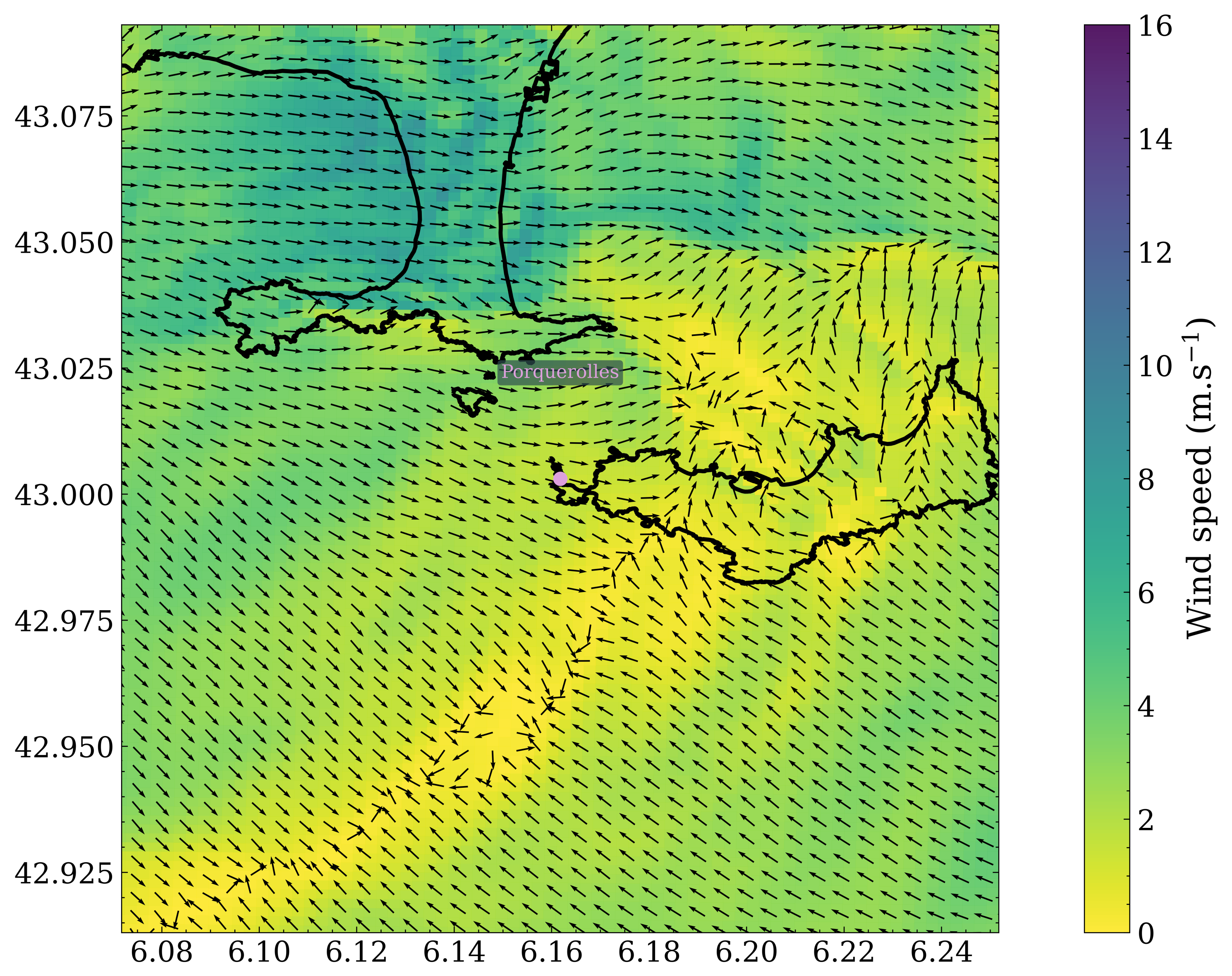
3.2. Spatial Discrepancies in Air Flow Patterns

The analysis of wind direction provides further insights into the spatial accuracy of the Meso-NH model simulations compared to actual meteorological conditions. An important observation regarding the comparison between the LES meteorological model and measured wind fields can also be made. In few cases, the wind direction locally measured on board or on the island of Porquerolles does not match with the one calculated by the model as reported, for instance in Figure 4, Figure 5 and Figure 6. In particular, if we noted that the LES model predicts well the occurrence of a wind front, the wind speed and direction measured locally demonstrates it does not coincide with exact location of the phenomenon above the sea surface, that is to say there is a spatial shift between measured and modeled wind values. This indicates that while LES models excel in capturing smaller vortices, as evident in Figure 4b, they may not fully account for the shift in the frontal zone, which significantly impacts the comparison with kilometric simulations. For instance, in few cases (i.e., points 7 and 6 in Figure 1), the ship was located close to or in the theoretical area of the wind field re-circulation, as calculated by the model, while it was clear that the local wind speed and direction measured in situ correspond to another area of the wind field. As an example, this can be observed in Figure 8 and Figure 9, where are reported zooms on Figure 5 and Figure 6. Figure 8 provides a detailed view of the eastern part of Figure 5b and Figure 9 focuses on the western section of Figure 6b. Figure 8 shows the Porquerolles measurement site and Figure 9 shows the position of the ship on board which the wind speed and direction plotted in Figure 7 were recorded. In Figure 8, the ship was positioned in a region where the wind direction was determined to be southeast, conflicting with the westward wind measurements taken on board. This discrepancy suggests that the frontal zone may have been located further west than previously modeled near Porquerolles island. This observation is corroborated by point 5 of Figure 10, where local measurements of wind speed and direction indicate that the front, although visible on Figure 8, is actually located further west than modeled. In addition, Figure 9 shows that close to the extreme west of the island of Porquerolles, we can observe a convergence zone between west and easterly winds resulting in the generation of a small eddy, which is well-captured by the finer grid. However, upon examining the wind direction locally measured at the Porquerolles station, we can note that this comes from the east, whereas the model predicts a west wind. Another discrepancy can be observed in Figure 9 which zoom on the western portion of Figure 6b. The ship is in zone where the model predicts an east direction whereas the direction was measured northwest on board. These results indicate that the wind re-circulation area is not accurately located by the model. Along the coast, the effective resolution is likely insufficient to solve sub-mesh processes, especially when the wind field spans both land and sea.
This is confirmed by Figure 10 wich depicts the wind directions, the wind directions predicted by the LES model are shown in yellow, those from the mesoscale model are depicted in blue and the actual measurements are denoted by purple arrows. The observations are grouped at the top for the Porquerolles station and at the bottom for the MIRAMER campaign. The ship positions are denoted by numbers from 1 to 17 in the x-axis.

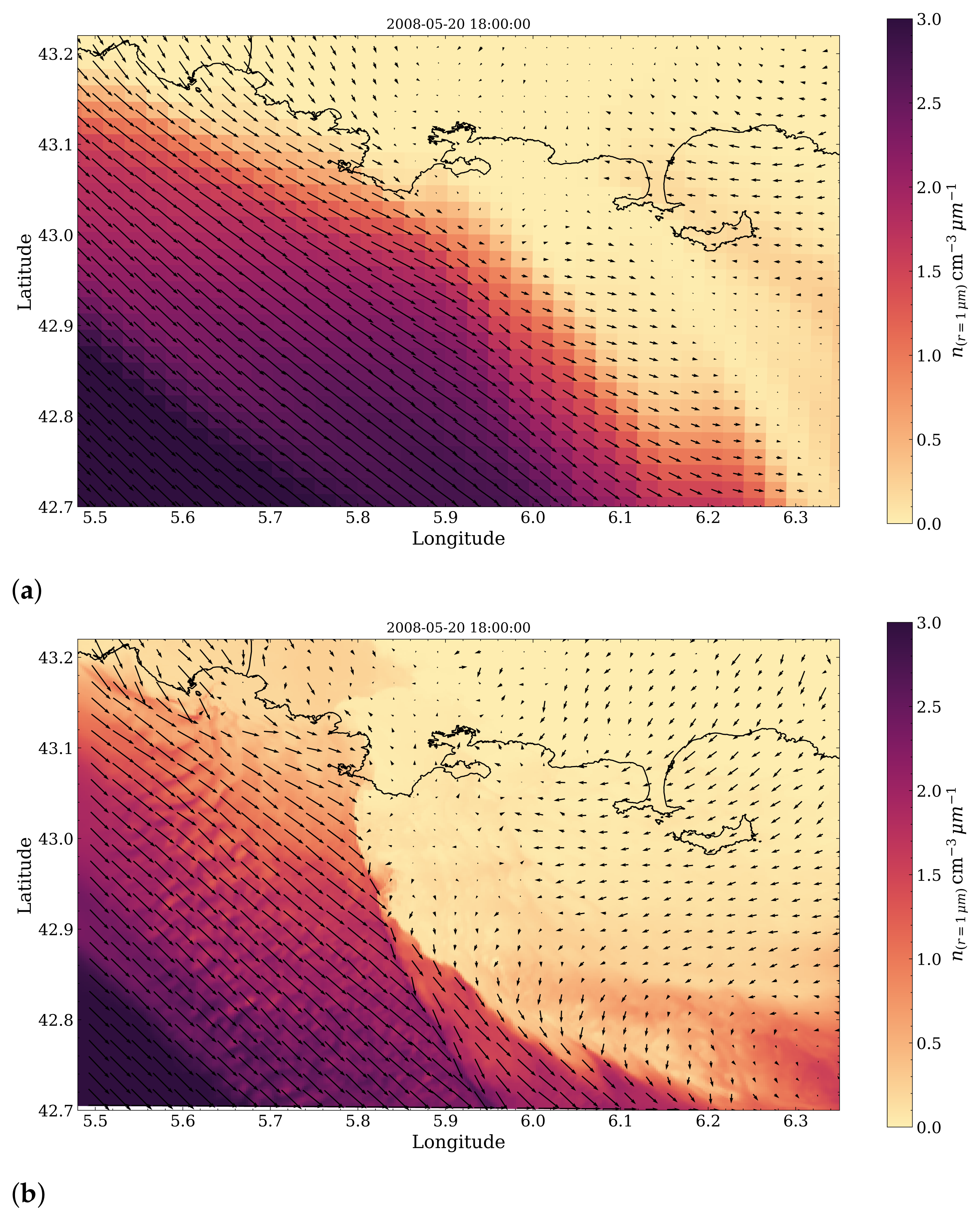
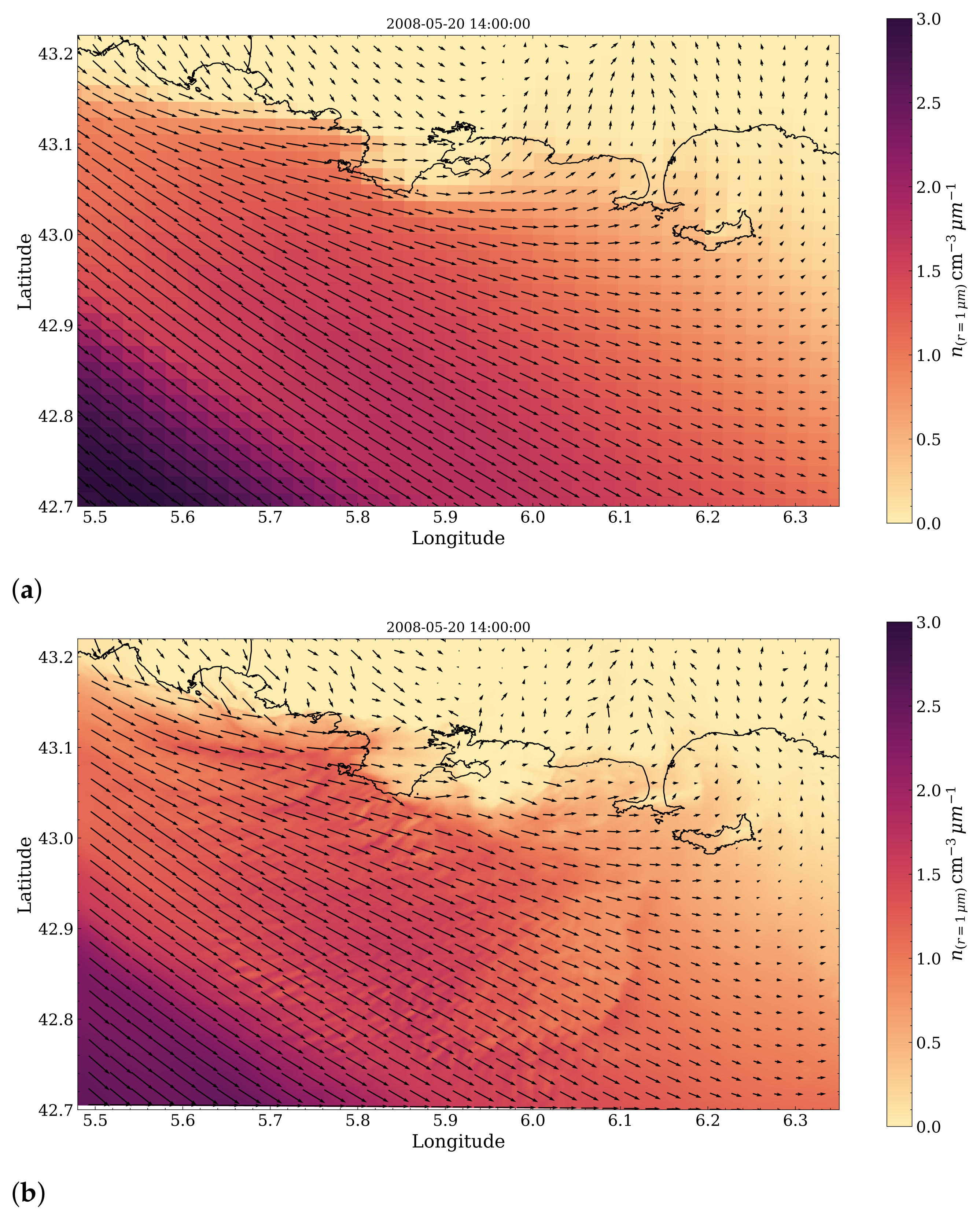
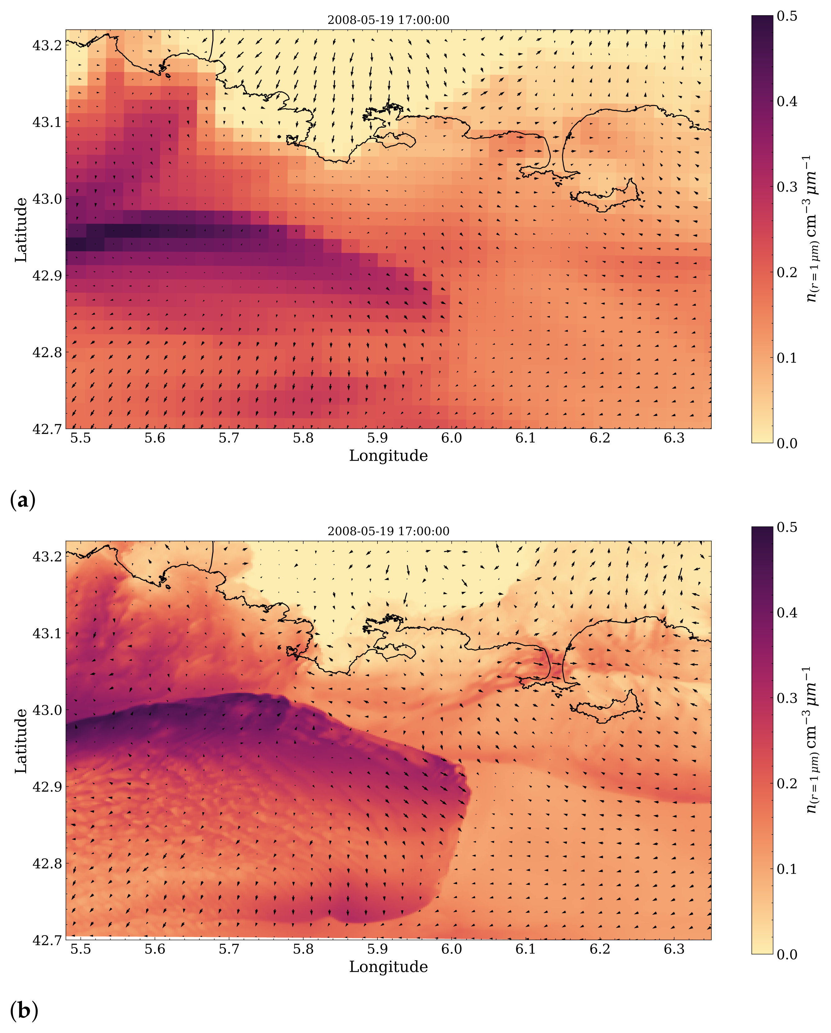
3.3. Sea-Spray Dynamics

Now that we have examined the performance of the Meso-NH model for capturing the wind field, we turn our attention to the aerosols. Having implemented the B21 formulation for sea-spray source function as described in Section 3 in the Meso-NH model, we propose a comparison between the spatio-temporal R/V Atalante.
Figure 11, Figure 12 and Figure 13 show the Meso-NH (top panels) and the Meso-NH-LES (bottom panels) simulations of the horizontal wind field and concentrations of 1 µm sea-spray droplets for the three examples already reported in Figure 4, Figure 5 and Figure 6, which correspond to typical meteorological episodes characteristic of the Toulon bay. Figure 11, Figure 12 and Figure 13 allow observation of the details of the spatio-temporal variation of sea-spray concentrations in the study area. During episodes of wind front convergence, or re-circulation, or local-scale atmospheric eddies, as observed for the wind field in Figure 4, Figure 5 and Figure 6, we do not observe in Figure 11, Figure 12 and Figure 13 the occurrence of sea-spray accumulation zones, as might be expected. Indeed, small vortexes in the atmospheric turbulent flow should “trap” a certain amount of aerosol resulting in peaks of concentrations, e.g., near the front zone. The finer grid size of the high-resolution LES model allows to capture small-scale atmospheric flows (Figure 4, Figure 5 and Figure 6) and as a result, the high-resolution simulations should detail aerosol-accumulation areas. However, this expected pattern is not observed in Figure 11, Figure 12 and Figure 13. The model seems to respond primarily to the processes of freshly generated particle emissions via air–sea interactions, rather than to the atmospheric transport of “aged” particles. This is confirmed by Figure 11, which shows a noticeable decrease in the sea-spray concentrations close to the Cepet Cap.
To assess whether the fine-scale details provided by the high-resolution model allow accurate determination of aerosol intrusion towards the continent, we have plotted Figure 14, which shows the relative difference between modeled and observed sea-spray concentrations for selected radii 1 µm and 2.5 µm. These particular radii were chosen as representative of sea-spray [39,59]. Figure 14 is dedicated to case studies demonstrating agreement between the LES calculations and the data in terms of wind speed and direction, as reported in Section 4. The data were recorded for different mean wind speeds on board the R/V Atalante and the simulations were derived from the LES model. Each point plotted in Figure 14 is calculated from approximately ten concentration values. Considering the results obtained in Section 3.1, the comparison is more specifically focused on the meteorological episodes for which the LES model outputs show good agreement with the wind data, i.e., ξ > 2000 and particularly during periods of high wind speeds that conduce to sea-spray production.
In contrast with the results reported for wind speed, discrepancies between LES simulations and experiments emerge for data dealing with the variation of the non-dimensional fetch ξ < 10,000 , whereas it was only for ξ < 2000 for the wind speed. In few cases, the aerosol concentration can vary by a factor of 3. Given that the wind speed was reasonably well-modeled by the model as outlined above (see Section 3.1), these differences are attributable to the formulation of the sea-spray source function rather than to discrepancies in the meteorological model outputs. The model struggles to accurately predict concentrations for low wind speed periods, sometimes coinciding with the presence of a frontal line and resulting in a very short fetch. It is important to note an exception for point 14, which even in cases of long fetch a significant errors occur. This arises under very stable conditions where it is known that the model is not particularly effective. Firstly, it is likely that the B21 source function formulation is less accurate for short fetches, which are associated with younger waves and unsteady conditions compared to remote ocean conditions. Younger waves are characterized by periods of wave energy amplification [28] variations, but may not grow enough to break, leading to negligible production of sea-spray aerosols. It is well-established that sea states can differ significantly depending on whether the wind fetch and duration are substantial or not at the same wind speed. The aerosol source function in Meso-NH depends on the wave slope (see Section 3) and in the B21 model, the determination of the wave slope is made using a linear function of the wind speed (see Equation (4)), which is likely more suitable for steady-state wave fields resulting from large fetch conditions. Consequently, for short fetches, the B21 formulation may either overestimate or underestimate atmospheric sea-spray concentrations. To verify this, we have calculated the relative difference between the measured wave slope using the buoy south of the island of Porquerolles (Figure 1) and the calculated wave slope using Equation (4). It is noticeable that during the campaign, the wave slope is, most of the time, underestimated by the model, which could partially explain why the performance of the LES model decreases under these conditions.

4. Discussion and Conclusions

The comparison of the outputs of the Meso-NH model and its LES version, to both meteorological and aerosol data, collected during the R/V Atalante measurement campaign, showed spatial shift of the atmospheric structures between the measurements and the model outputs. This is a numerical model shortcoming in agreement with previous studies in the literature, e.g., Canepa et al. [60] and Yu et al. [61]. The main interest of the data acquired on board the R/V Atalante during the Miramer campaign is the possibility to have in situ data at various fetches. This kind of ship measurements is rather rare.
Firstly, since wind speed is a key parameter for many physical and chemical processes related to climate properties, including the generation and atmospheric transport of sea-spray aerosols, a comparison between the in situ measured wind speed and the model calculations has been presented in Section 3.1. Our results indicate that high-resolution numerical modeling, in the majority of the cases, provides more accurate predictions accurate predictions for velocity fields. From the meteorological perspective, we observed that the LES resolution offers finer details and captures turbulent features that the mesoscale resolution might overlook, especially very near the coast. We indeed observed that the two models, i.e., mesoscale and LES, compare favorably for wind speed at a relatively great distance from the coast, particularly for a non-dimensional fetch > 10,000. However, the two methodologies were observed to differ for non-dimensional fetches between 2000 and 10,000, highlighting the importance of wind direction in coastal areas. In these instances, the LES resolution ability to capture turbulent features of the wind field that the mesoscale resolution might miss, such as wind re-circulation cells due to the presence of coasts or the occurrence of fronts, was noted. As a result, a higher accuracy of the LES model in predicting wind speed is observed. However, for fetches < 2000, which may involve a wind trajectory alternating between ocean surface and land before reaching the measurement station, the LES outputs show limitations. At very short fetches, the increased resolution provided by the LES model does not guarantee improved precision in reproducing the wind field. Specifically, the model does not accurately predict wind re-circulation phenomena at their actual marine surface locations. Along the coast, the effective resolution is not sufficient to resolve sub-mesh processes, particularly when the wind field spans both land and sea. Perhaps a finer resolution is required, but this would need to be balanced with computational time constraints. For meteorological episodes where the LES model under performs, it was noted that with regard to wind direction, the ship was located in the land-sea transition zone characterized by a very short fetch. Additionally, significant errors between LES model simulations and wind data were observed during episodes of very stable atmospheric conditions.
If the results outlined above confirm the good performance of the LES version of the Meso-NH model in representing meteorological parameters near the coast, its accuracy for sea-spray concentration calculations is more questionable. The present results clearly show that the model performance is contingent on the choice of the sea-spray source function formulation implemented. Firstly, during episodes of wind front convergence or the presence of re-circulation or local-scale atmospheric eddies as observed in Figure 4, Figure 5 and Figure 6, we do not observe the expected sea-spray-accumulation zones. Given the ability of the LES model finer grid size to capture small-scale atmospheric flows, high-resolution simulations should clearly reveal areas of aerosol accumulation and aerosol intrusions over the continent. Therefore, it is evident that fine-scale details of the aerosol concentration patterns are not well-resolved, even by the high-resolution model. While our results confirm the accuracy of using B21 in open ocean [35], this study underscores the need for subtle adjustments to the source function when dealing with short fetch, especially near the coastline. Additionally, the weight of freshly produced aerosols in the concentrations calculated by the model seems greater than that of aged aerosols. This highlights the limitations in capturing fine-scale turbulent features crucial for precise aerosol modeling, particularly in the land-sea transition zone. The current study does not include a coupling between wave dynamics and wind, which could potentially refine the representation of wave behavior based on local wind conditions. Such a coupling might provide a more accurate description of the marine environment and enhance predictions of aerosol dynamics, especially in complex coastal settings. Reducing to lower resolutions is an important computational challenge in terms of computing issues. The computational cost and time required for a refinement process are challenges that will be addressed in the future development of our work.
The fetch is a pivotal parameter in coastal zones. The fetch, defined as the distance an air mass has traveled over water without variations, is an additional relevant apt descriptor for aerosol dynamics in coastal zones [39], as it accounts for the build-up of marine aerosol concentrations as the air mass moves over the sea. It provides more comprehensive information than locally calculated wave age and significantly influences the characteristics and transport of sea-spray aerosols.If the wind direction remains constant, a longer fetch and higher wind speed transfer more wind energy to the water surface, resulting in a larger sea state. The spatio-temporal variation of sea-spray in the study area provided by the LES model corresponds closely with experimental data acquired on board the R/V Atalante for fetches > 10,000. This is primarily due to the limitations of the sea-surface source function, which struggles to accurately describe spatial and temporal variations in aerosol concentrations in coastal areas. These shortcomings mainly arise from the imprecision of the source function formulation used during the campaign. It should be noted that different acquisition systems for aerosols result in a significant variety of data, such as mass concentrations, number concentrations, PM10 and PM2.5. The quality of these datasets must be checked before they are used in an assimilation framework. Additionally, in urban zones, a variety of aerosol sources coexist and there is a lack of information necessary for editing relevant emission inventories. The number of unknowns in the problem of atmospheric aerosol dispersion persist.
In conclusion, while specific cases of error, in terms of geographical locations and wind direction, persists between wind data and LES simulations, the present paper highlights the additional benefits offered by higher resolution. Our results also underscore the considerable challenge of developing an accurate CTM model for sea-spray dynamics, especially in regions with complex topography and varied surface types, as often encountered in coastal areas.

Supplementary Materials

The following supporting information can be downloaded at: https://www.mdpi.com/article/10.3390/atmos15060702/s1.

Author Contributions

Conceptualization, A.L., J.P. and E.C.; methodology, A.L. and J.P.; software, A.L. and C.Y.; validation, A.L., J.P. and Q.R.; formal analysis, A.L. and J.P.; investigation, A.L.; resources, Q.R. and C.Y.; data curation, W.B.; writing—original draft preparation, J.P.; writing—review and editing, A.L., P.S., E.C. and J.P.; visualization, A.L.; supervision, J.P. and P.S.; project administration, J.P.; funding acquisition, P.S. All authors have read and agreed to the published version of the manuscript.

Funding

This work was sponsored by ANR-ASTRID under contract ANR-18-ASTR-0002.

Institutional Review Board Statement

Not applicable.

Informed Consent Statement

Not applicable.

Data Availability Statement

The data presented in this study are available on request from the corresponding author. The data are not publicly available due to privacy.

Conflicts of Interest

The authors declare no conflicts of interest.

References

  1. Charlson, R.J.; Schwartz, S.E.; Hales, J.M.; Cess, R.D.; Coakley, J.A., Jr.; Hansen, J.E.; Hoffman, D.J. Climate forcing by anthropogenic aerosols. Science 1992, 255, 423–430. [Google Scholar] [CrossRef] [PubMed]
  2. Mason, B.J. The role of sea-salt particles as cloud condensation nuclei over the remote oceans. Q. J. R. Meteorol. Soc. 2001, 127, 2023. [Google Scholar] [CrossRef]
  3. Andreae, M.O. Climate effects of changing atmospheric aerosol levels. World Surv. Climatol. 1995, 16, 341–392. [Google Scholar]
  4. Jaenicke, R. Physical aspects of atmospheric aerosol. In Aerosols and Their Climatic Effects; Gerbard, H., Deepak, A., Eds.; Deepak Publishing: Hampton, VA, USA, 1984; pp. 7–34. [Google Scholar]
  5. Yoon, Y.; O’Dowd, C.; Jennings, S.; Lee, S. Statistical characteristics and predictability of particle formation events at Mace Head. J. Geophys. Res. 2006, 111, D13204. [Google Scholar] [CrossRef]
  6. Mallet, M.; Roger, J.; Despiau, S.; Dubovik, O.; Putaud, J. Microphysical and optical properties of aerosol particles in urban zone during ESCOMPTE. Atmos. Res. 2003, 69, 73–97. [Google Scholar] [CrossRef]
  7. Mulcahy, J.; O’Dowd, C.; Jennings, S.; Ceburnis, D. Significant enhancement of aerosol optical depth in marine air under high wind conditions. Geophys. Res. Lett. 2008, 35. [Google Scholar] [CrossRef]
  8. Lewis, E.; Lewis, R.; Karlstrom, K.; Schwartz, S. Sea Salt Aerosol Production: Mechanisms, Methods, Measurements, and Models; American Geophysical Union: Washington, DC, USA, 2004; Volume 152. [Google Scholar]
  9. Piazzola, J.; Mihalopoulos, N.; Canepa, E.; Tedeschi, G.; Prati, P.; Zarmpas, P.; Bastianini, M.; Missamou, T.; Cavaleri, L. Characterization of aerosols above the Northern Adriatic Sea: Case studies of offshore and onshore wind conditions. Atmos. Environ. 2016, 132, 153–162. [Google Scholar] [CrossRef]
  10. Johansson, J.; Salter, M.; Navarro, J.; Leck, C.; Nilsson, E.; Cousins, I. Global transport of perfluoroalkyl acids via sea-spray aerosol. Environ. Sci. Proc. Impacts 2019, 21, 635–649. [Google Scholar] [CrossRef] [PubMed]
  11. Gustafsson, M.; Franzen, L. Dry deposition and concentration of marine aerosols in a coastal area; SW Sweden. Atmos. Environ. 1996, 30, 977–989. [Google Scholar] [CrossRef]
  12. Farrell, E. Atmospheric deposition in maritime environments and its impact on terrestrial ecosystems. Water Air Soil Pollut. 1995, 1, 1573–2932. [Google Scholar] [CrossRef]
  13. Monahan, E.; Spiel, D.; Davidson, K. A model of marine aerosol generation via whitecaps and wave disruption. In Oceanic Whitecaps; Monahan, E., McNiocaill, G., Eds.; D. Reidel: Norwell, MA, USA, 1986; pp. 167–174. [Google Scholar]
  14. Blanchard, D.C. The Ejection of Drops from the Sea and Their Enrichment with Bacteria and Other Materials: A Review. Estuaries 1989, 12, 127–137. [Google Scholar] [CrossRef]
  15. Spiel, D.E. Formation and production of sea-spray aerosol. J. Aerosol Sci. 1996, 27, S65–S66. [Google Scholar] [CrossRef]
  16. Van Eijk, A.; Kusmierczyk-Michulec, J.; Francius, M.; Tedeschi, G.; Piazzola, J.; Meritt, D.; Fontana, J. Sea-spray aerosol particles generated in the surf zone. J. Geophys. Res. 2011, 116, D19210. [Google Scholar] [CrossRef]
  17. O’Dowd, C.D.; de Leeuw, G. Marine aerosol production: A review of the current knowledge. Phil. Trans. R. Soc. A 2007, 365, 1753–1774. [Google Scholar] [CrossRef] [PubMed]
  18. Andreas, E. Sea spray and the turbulent air-sea heat fluxes. J. Geophys. Res. 1992, 97, 11429–11441. [Google Scholar] [CrossRef]
  19. Emanuel, K. Tropical Cyclone Activity Downscaled from NOAA-CIRES Reanalysis; 1908–1958. J. Adv. Model. Earth Syst. 2010, 2, 1942–2466. [Google Scholar] [CrossRef]
  20. Tsyro, S.; Aas, W.; Soares, J.; Sofiev, M.; Berge, H.; Spindler, G. Modelling of sea salt concentrations over Europe: Key uncertainties and comparison with observations. Atmos. Chem. Phys. 2011, 11, 10367–10388. [Google Scholar] [CrossRef]
  21. Chen, Y.; Cheng, Y.; Ma, N.; Wolke, R.; Nordmann, S.; Schüttauf, S.; Ran, L.; Wehner, B.; Birmili, W.; Gon, H.; et al. Sea salt emission, transport and influence on size-segregated nitrate simulation: A case study in northwestern europe by WRF-Chem. Atmos. Chem. Phys. 2016, 16, 12081–12097. [Google Scholar] [CrossRef]
  22. Neumann, D.; Matthias, V.; Bieser, J.; Aulinger, A.; Quante, M. A comparison of sea salt emission parameterizations in northwestern Europe using a chemistry transport model setup. Atmos. Chem. Phys. 2016, 16, 9905–9933. [Google Scholar] [CrossRef]
  23. Xingkun, X.; Voermans, J.; Moon, I.J.; Babanin, A. Sea Spray Impacts on Tropical Cyclone Olwyn Using a Coupled Atmosphere-Ocean-Wave Model. J. Geophys. Res. Oceans 2022, 127. [Google Scholar] [CrossRef]
  24. Aouizerats, B.; Tulet, P.; Pigeon, G.; Masson, V.; Gomes, L. High resolution modelling of aerosol dispersion regimes during the CAPITOUL field experiment: From regional to local scale interactions. Atmos. Chem. Phys. 2011, 11, 7547–7560. [Google Scholar] [CrossRef]
  25. Delbeke, L.; Wang, C.; Tulet, P.; Denjean, C.; Zouzoua, M.; Maury, N.; Deroubaix, A. The impact of aerosols on stratiform clouds over southern West Africa: A large-eddy-simulation study. Atmos. Chem. Phys. 2023, 23, 13329–13354. [Google Scholar] [CrossRef]
  26. Laussac, S.; Piazzola, J.; Tedeschi, G.; Yohia, C.; Canepa, E.; Rizza, U.; Van Eijk, A. Development of a fetch dependent sea-spray source function using aerosol concentration measurements in the north-western Mediterranean. Atmos. Environ. 2018, 193, 177–189. [Google Scholar] [CrossRef]
  27. Tedeschi, G.; Piazzola, J. Development of a 2D marine aerosol transport model: Application to the influence of thermal stability in the marine atmospheric boundary layer. Atmos. Res. 2011, 101, 469–479. [Google Scholar] [CrossRef]
  28. Lafon, C.; Piazzola, J.; Le Calve, O.; Forget, P.; Despiau, S. Analysis of the variations of the whitecap fraction as measured in a coastal zone during the FETCH experiment. Boundary-Layer Meteorol. 2004, 111, 339–360. [Google Scholar] [CrossRef]
  29. Parent, P.; Laffon, C.; Trillaud, V.; Grauby, O.; Ferry, D. Physicochemical Characterization of Aerosols in the Coastal Zone: Evidence of Persistent Carbon Soot in the Marine Atmospheric Boundary Layer (MABL) Background. Atmosphere 2023, 14, 291. [Google Scholar] [CrossRef]
  30. Liu, F.; Peng, L.; Dai, S.; Bi, X.; Shi, M. Size-Segregated Characteristics of Organic Carbon (OC) and Elemental Carbon (EC) in Marine Aerosol in the Northeastern South China Sea. Atmosphere 2023, 14, 661. [Google Scholar] [CrossRef]
  31. Piazzola, J.; Bruch, W.; Desnues, C.; Parent, P.; Yohia, C.; Canepa, E. Influence of Meteorological Conditions and Aerosol Properties on the COVID-19 Contamination of the Population in Coastal and Continental Areas in France: Study of Offshore and Onshore Winds. Atmosphere 2021, 12, 523. [Google Scholar] [CrossRef]
  32. Stifanese, R.; Canepa, E.; Traverso, P. Corrosion of 316L Stainless Steel used for Building Applications in Marine–Urban Atmospheres: A Case Study from Genoa, Italy. J. Archit. Eng. 2022, 28. [Google Scholar] [CrossRef]
  33. Jeon, D.; Jung, J.; Park, J.; Min, J.; Oh, J.E.; Moon, J.; Lee, J.S.; Yoon, S. Predicting airborne chloride deposition in marine bridge structures using an artificial neural network model. Constr. Build. Mater. 2022, 337, 127623. [Google Scholar] [CrossRef]
  34. Bruch, W.; Piazzola, J.; Branger, H.; Luneau, C.; Bourras, D.; Tedeschi, G.; van Eijk, A. Spray Production Dependence on Wind and Wave Combinations: A Tunnel Study. Bound.-Layer Meteorol. 2021, 180, 477–505. [Google Scholar] [CrossRef]
  35. Bruch, W.; Yohia, C.; Tulet, P.; Limoges, A.; Sutherland, P.; van Eijk, A.; Missamou, T.; Piazzola, J. Atmospheric Sea Spray Modeling in the North-East Atlantic Ocean Using Tunnel-Derived Generation Functions and the SUMOS Cruise Dataset. J. Geophys. Res. 2023, 128, e2022JD038330-23p. [Google Scholar] [CrossRef]
  36. Lac, C.; Chaboureau, J.P.; Masson, V.; Pinty, J.P.; Tulet, P.; Escobar, J.; Leriche, M.; Barthe, C.; Aouizerats, B.; Augros, C.; et al. Overview of the Meso-NH model version 5.4 and its applications. Geosci. Model Dev. 2018, 11, 1929–1969. [Google Scholar] [CrossRef]
  37. Honnert, R.; Masson, V.; Lac, C. A Theoretical Analysis of Mixing Length for Atmospheric Models From Micro to Large Scales. Front. Earth Sci. 2021, 8, 582056. [Google Scholar] [CrossRef]
  38. Hsu, S. A mechanism for the increase of wind stress (drag) coefficient with wind speed over water surfaces: A parametric model. J. Phys. Oceanogr. 1986, 16, 144–150. [Google Scholar] [CrossRef]
  39. Piazzola, J.; Despiau, S. Contribution of marine aerosols in the particle size distributions observed in Mediterranean coastal zone. Atm. Environ. 1997, 31, 2991–3009. [Google Scholar] [CrossRef]
  40. Brockmann, J. Sampling and Transport of Aerosols; Van Nostrand Reinhold: New York, NY, USA, 1993; pp. 77–111. [Google Scholar]
  41. Frick, G.; Hoppel, W. Airship measurements of ship’s exhaust plumes and their effect on marine boundary layer clouds. J. Atmos. Sci. 2000, 57, 2625–2648. [Google Scholar] [CrossRef]
  42. Savelyev, I.; Anguelova, M.; Frick, G.; Dowgiallo, D.; Hwang, P.; Caffrey, P.; Bobak, J. On direct passive microwave remote sensing of sea-spray aerosol production. Atmos. Chem. Phys. 2014, 14, 11611. [Google Scholar] [CrossRef]
  43. Limoges, A.; Yohia, C.; Rodier, Q.; van Eijk, A.; Piazzola, J. High-resolution modeling of the spatiotemporal variations in aerosol extinction in a complex coastal area. In Proceedings of the Environmental Effects on Light Propagation and Adaptive Systems VI, SPIE Remote Sensing, Amsterdam, The Netherlands, 3–7 September 2023; Volume 12731, p. 127310C. [Google Scholar] [CrossRef]
  44. Lunet, T.; Lac, C.; Auguste, F.; Visentin, F.; Masson, V.; Escobar, J. Combination of WENO and Explicit Runge–Kutta Methods for Wind Transport in the Meso-NH Model. Mon. Weather Rev. 2017, 145, 3817–3838. [Google Scholar] [CrossRef]
  45. Berger, A.; Barbet, C.; Leriche, M.; Deguillaume, L.; Mari, L.; Chaumerliac, C.; Bègue, N.; Tulet, P.; Gazen, D.; Escobar, J. Evaluation of Meso-NH. Atmos. Res. 2016, 176–177, 43–63. [Google Scholar] [CrossRef]
  46. Farr, T.G.; Rosen, P.A.; Caro, E.; Crippen, R.; Duren, R.; Hensley, S.; Kobrick, M.; Paller, M.; Rodriguez, E.; Roth, L.; et al. The Shuttle Radar Topography Mission. Rev. Geophys. 2007, 45, RG2004. [Google Scholar] [CrossRef]
  47. Redelsperger, J.; Sommeria, G. Method of representing the turbulence associated with precipitations in a three-dimensional model of cloud convection. Bound. Layer Meteorol. 1982, 24, 231–252. [Google Scholar] [CrossRef]
  48. Redelsperger, J.; Sommeria, G. Three-dimensional simulation of a convective storm: Sensitivity studies on subgrid parameterization and spatial resolution. J. Atmos. Sci. 1986, 43, 2619–2635. [Google Scholar] [CrossRef]
  49. Cuxart, J.; Bougeault, P.; Redelsperger, J. A turbulence scheme allowing for mesoscale and large-eddy simulations. Q. J. R. Meteorol. Soc. 2000, 126, 1–30. [Google Scholar] [CrossRef]
  50. Cheng, Y.; Canuto, V.M.; Howard, A.M. An improved model for the turbulent PBL. J. Atmos. Sci. 2002, 59, 1550–1565. [Google Scholar] [CrossRef]
  51. Bougeault, P.; Lacarrere, P. Parameterization of Orography-Induced Turbulence in a Mesobeta–Scale Model. Mon. Weather Rev. 1989, 117, 1872–1890. [Google Scholar] [CrossRef]
  52. Ovadnevaite, J.; de Leeuw, G.; Ceburnis, D.; Monahan, C.; Partanen, A.I.; Korhonen, H. A sea-spray aerosol flux parameterization encapsulating wave state. Atmos. Chem. Phys. 2014, 14, 1837–1852. [Google Scholar] [CrossRef]
  53. Cox, C.; Munk, W. Measurement of the roughness of the sea surface from photographs of the sun’s glitter. Josa 1954, 44, 838–850. [Google Scholar] [CrossRef]
  54. Bréon, F.; Henriot, N. Spaceborne observations of ocean glint reflectance and modeling of wave slope distributions. J. Geophys. Res. 2006, 111. [Google Scholar] [CrossRef]
  55. Lenain, L.; Statom, N.; Melville, W. Airborne measurements of surface wind and slope statistics over the ocean. J. Phys. Oceanogr. 2019, 49, 2799–2814. [Google Scholar] [CrossRef]
  56. Bentamy, A.; Croize-Fillon, D.; Perigaud, C. Characterization of ASCAT measurements based on buoy and QuikSCAT wind vector observations. Ocean Sci. 2008, 4, 265–274. [Google Scholar] [CrossRef]
  57. Ricard, D.; Lac, C.; Riette, S.; Legrand, R.; Mary, A. Kinetic energy spectra characteristics of two convection-permitting limited-area models AROME and Meso-NH. Q. J. R. Meteorol. Soc. 2013, 139, 1327–1341. [Google Scholar] [CrossRef]
  58. Rodier, Q.; Masson, V.; Couvreux, F.; Paci, A. Evaluation of a Buoyancy and Shear Based Mixing Length for a Turbulence Scheme. Front. Earth Sci. 2017, 5, 65. [Google Scholar] [CrossRef]
  59. Van Eijk, A.; De Leeuw, G. Modeling aerosol particle size distributions over the North sea. J. Geophys. Res. 1992, 97, 14417–14429. [Google Scholar] [CrossRef]
  60. Canepa, E.; Irwin, J. Evaluation of air pollution models. In Air Quality Modeling—Theories, Methodologies, Computational Techniques, and Available Databases and Software; Zannetti, P., Ed.; The EnviroComp Institute and Air & Waste Management Association: Fremont, CA, USA, 2005; Volume II—Advanced Topics, pp. 503–556. [Google Scholar]
  61. Yu, W.; Nakakita, E.; Kim, S.; Yamaguchi, K. Assessment of Ensemble Flood Forecasting with Numerical Weather Prediction by considering Spatial Shift of Rainfall Fields. KSCE J. Civ. Eng. 2018, 22, 3686–3696. [Google Scholar] [CrossRef]
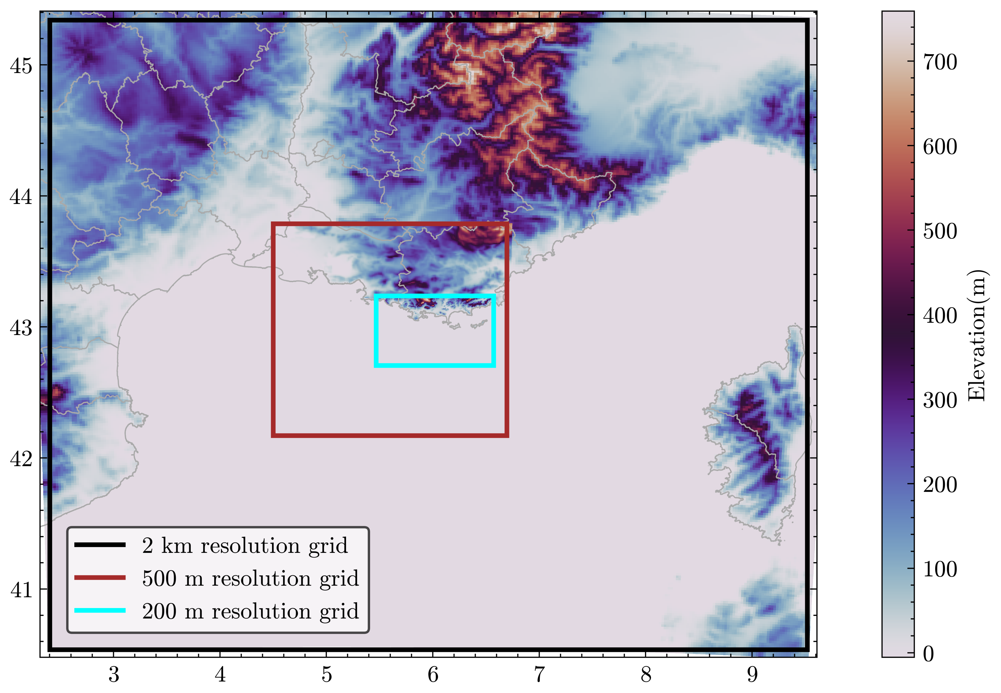
Figure 1. General view of the study area, as well as the calculation domain used for the Meso-NH calculations. The numbered stars show stops of the R/V Atalante for aerosol and meteorological data acquisition. The location of the buoy is marked by a green symbol.
Atmosphere 15 00702 g001
Figure 2. Foremast view (right, courtesy of Peter Sutherland–LOPS) and top view of the R/V Atalante (left).
Atmosphere 15 00702 g002
Figure 3. Adjusted orography for the domains used in this study—D01 at 2 km spatial grid (black square), D02 at 500 m spatial grid (red) and D03 (LES) at 200 m (blue).
Atmosphere 15 00702 g003
Figure 4. Wind field calculated for 20 May at 6 p.m. using the Meso-NH model. Panel (a) shows the simulations made using kilometric resolution, (b) the LES calculations and (c) the relative difference in wind speed calculated by the two models. Note: The arrows indicating wind direction arrows do not indicate wind speed magnitude.
Atmosphere 15 00702 g004
Figure 5. Wind field calculated for the day of 20 May at 2 p.m. using the Meso-NH model where panel (a) shows the simulations made using the kilometric resolution, (b) the LES calculations and (c) the relative difference of the wind speed calculated by the two models. Note: The arrows indicating wind direction arrows do not indicate wind speed magnitude.
Atmosphere 15 00702 g005
Figure 6. Wind field calculated for the day of 19 May at 5 p.m. using the Meso-NH model. Panel (a) shows the simulations made using the kilometric resolution, (b) the LES calculations and (c) the relative difference of the wind speed calculated by the two models. Note: The arrows indicating wind directions are not proportional to wind speed.
Atmosphere 15 00702 g006
Figure 7. A comparison of the wind speed measurements taken on board the R/V Atalante (stars symbols) with the numerical simulations from both the mesoscale model (crosses) and the high-resolution model (bullets). The numbers on the x-axis correspond to the measurements points as shown in Figure 1. The colour of the stars indicates the calculated non-dimensional fetch (Equation (1)) as shown in the horizontal colour bar reported on the top of the figure. We also reported the wind direction recorded during each episode.
Atmosphere 15 00702 g007
Figure 8. Zoom on the west portion of Figure 5b. The pink dot indicates the location of the measurements. Note: The arrows indicating wind directions are not proportional to wind speed.
Atmosphere 15 00702 g008
Figure 9. Zoom on east portion of Figure 6b. The pink dot indicates the location of the measurements. Note: The arrows indicating wind directions are not proportional to wind speed.
Atmosphere 15 00702 g009
Figure 10. Comparison of wind directions from MNH mesoscale and MNH LES configurations with measurements at the Porquerolles site and for the MIRAMER campaign.
Atmosphere 15 00702 g010
Figure 11. Map of sea-spray concentration calculated using the MesoNH (a) and the MesoNH LES (b) model for the day of 20 May at 6 p.m.
Atmosphere 15 00702 g011
Figure 12. Map of sea-spray concentration calculated using the MesoNH (a) and the MesoNH LES (b) model for the day of 20 May at 2 p.m.
Atmosphere 15 00702 g012
Figure 13. Map of sea-spray concentration calculated using the MesoNH (a) and the MesoNH LES (b) model for the day of 19 May at 5 p.m.
Atmosphere 15 00702 g013
Figure 14. Difference between modeled and available observed aerosol concentrations, as measured on board the R/V Atalante, for selected radii of 1 µm (bullets) and 2.5 µm (crosses). Blue symbols correspond to non-dimensional fetch less than 10,000, red symbols correspond to non-dimensional fetch greater than 10,000.
Atmosphere 15 00702 g014
Table 1. Domain Specifications.
DomainGrid PointsApproximate Size (km)
2 km resolution grid302 × 2721108 × 928
500 m resolution grid182 × 182586 × 478
200 m resolution grid (LES)452 × 30291 × 60
Disclaimer/Publisher’s Note: The statements, opinions and data contained in all publications are solely those of the individual author(s) and contributor(s) and not of MDPI and/or the editor(s). MDPI and/or the editor(s) disclaim responsibility for any injury to people or property resulting from any ideas, methods, instructions or products referred to in the content.

