
Microclimate Zoning Based on Double Clustering Method for Humid Climates with Altitudinal Gradient Variations: A Case Study of Colombia
 , , , and
Abstract
:1. Introduction
1.1. Conceptualization
1.2. Climate Zoning Background
1.3. Aim and Contribution of This Study
- I.
- Introduce, using updated TMY and PDIR-Now, open-access climate files based on high-resolution satellite information (4.4 km pixel).
- II.
- Perform a double clustering for global and local climate zoning for an emerging country located in a tropical region influenced by altitudinal gradient based on seven climate parameters and three geographical parameters.
- III.
- A new climate classification based on multivariate analysis has been established for Colombia.
2. Existing Climate Zoning of Colombia
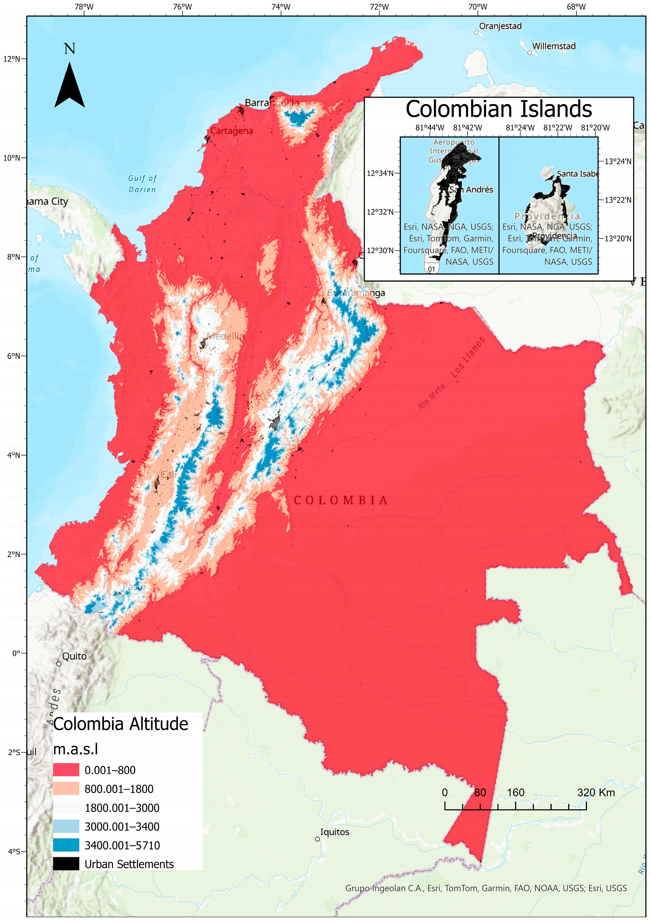
2.1. The Study Area
2.2. Climate Zoning of the Region
3. Materials and Methods
3.1. Boundary Conditions
3.2. Data Processing
- Daily cumulative GHI (W/m2)
- Daily average wind speed (m/s)
- Daily maximum and minimum relative humidity (%)
- Daily maximum and minimum dry-bulb temperature (°C)
- Daily cumulative rainfall (mm)
3.3. Clustering Analysis
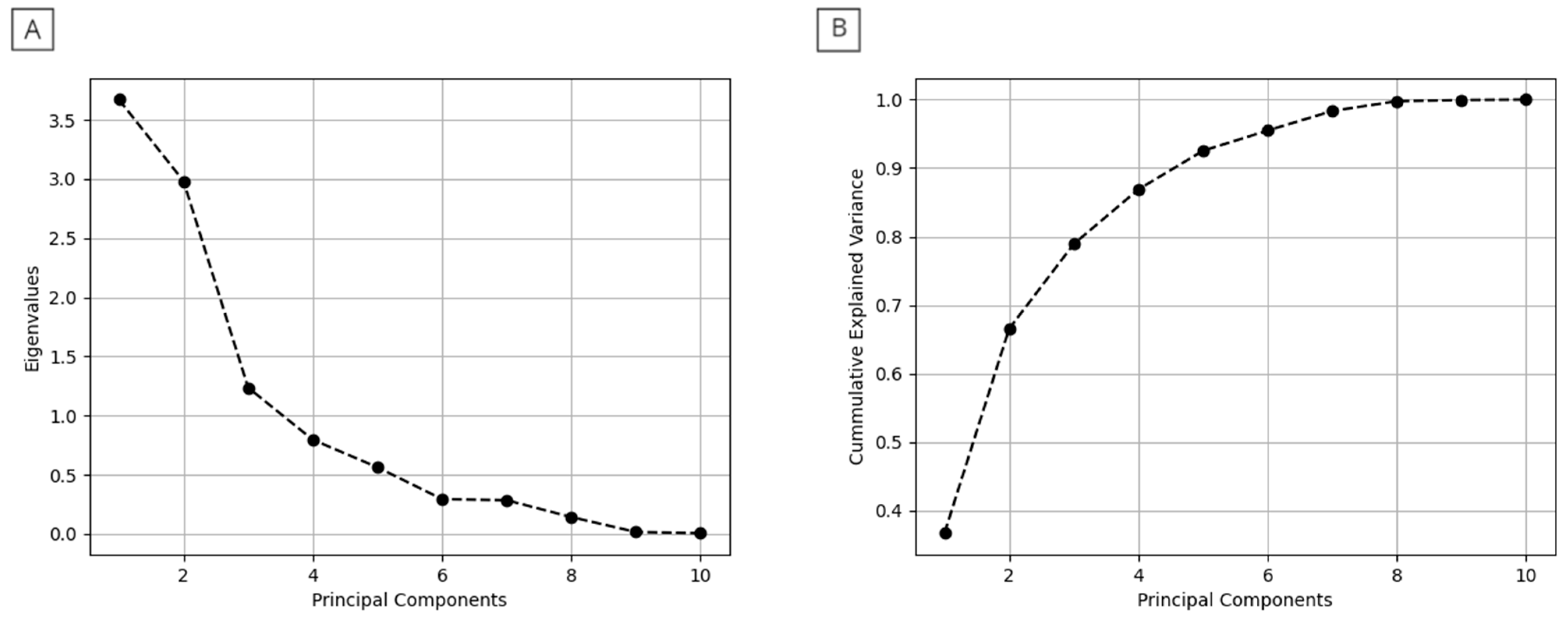
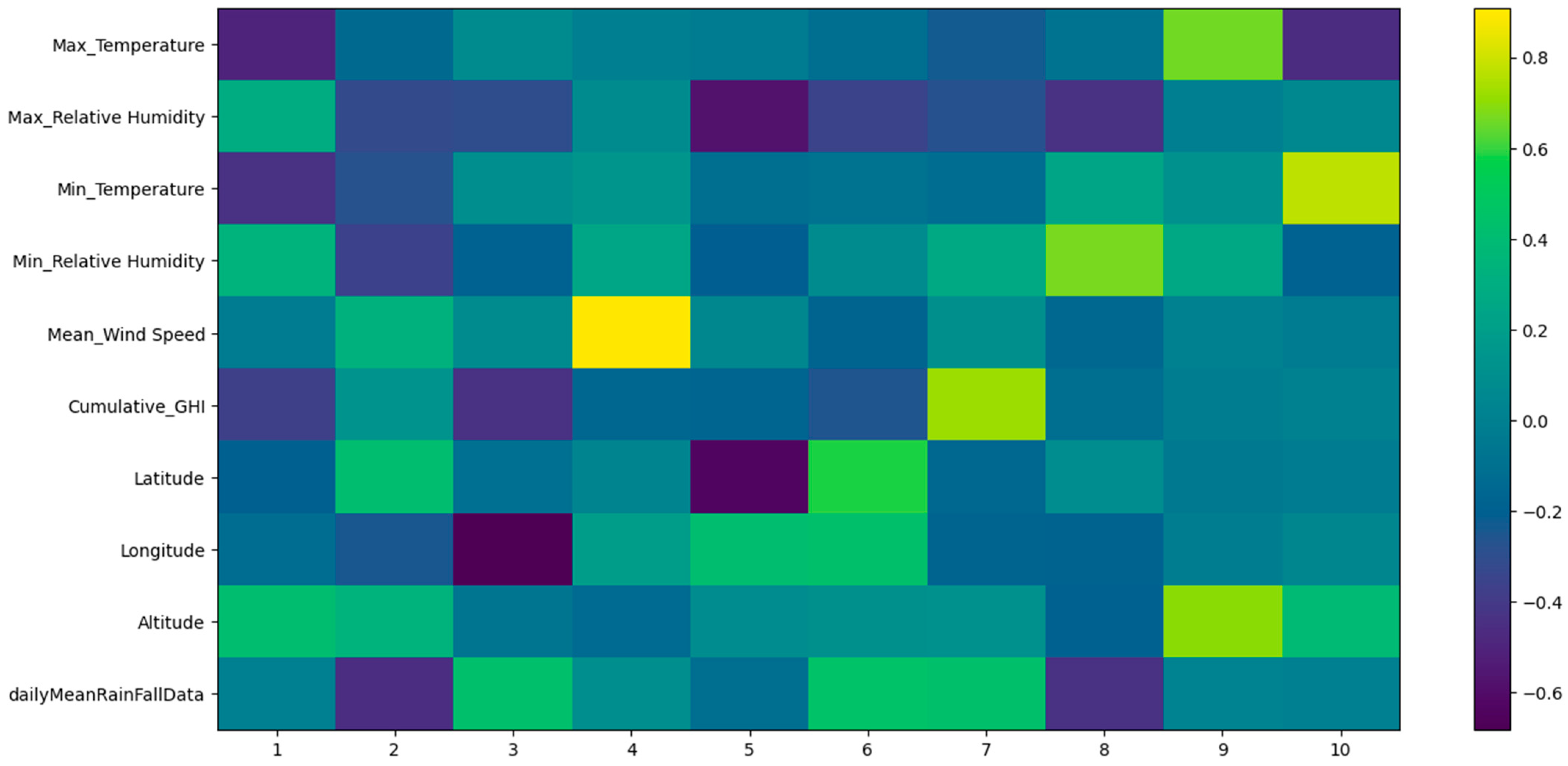
3.3.1. Principal Component Analysis (PCA)
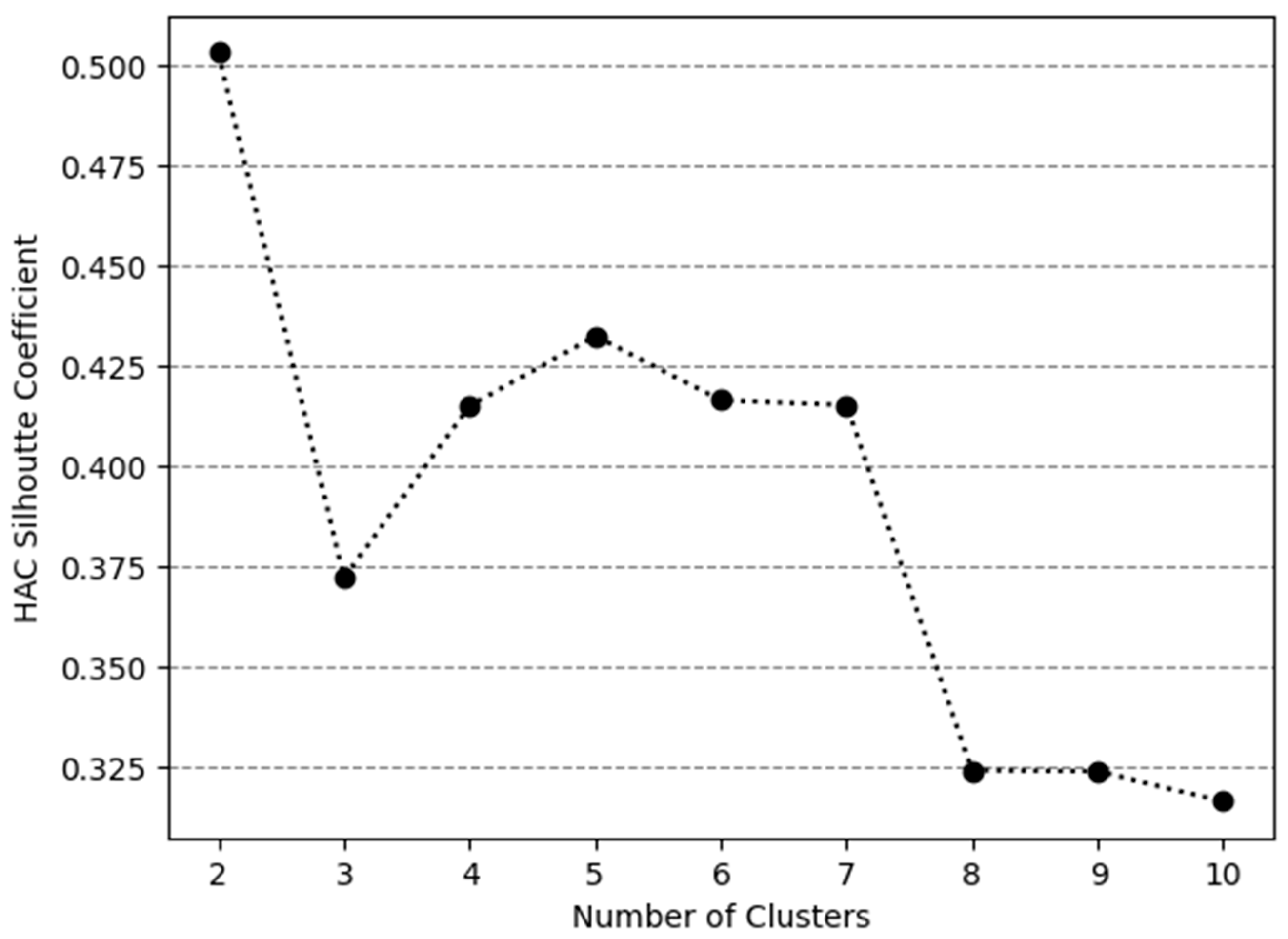
3.3.2. Hierarchical Clustering Analysis
- a represents the mean distance of a point and other points that belong to the same clusters,
- b represents the mean distance of a point and points that belong to the nearest cluster.
- is the distance between a point (p) and the cluster centroid (c) to which it belongs.
3.4. Spatial Distribution Mapping
4. Results
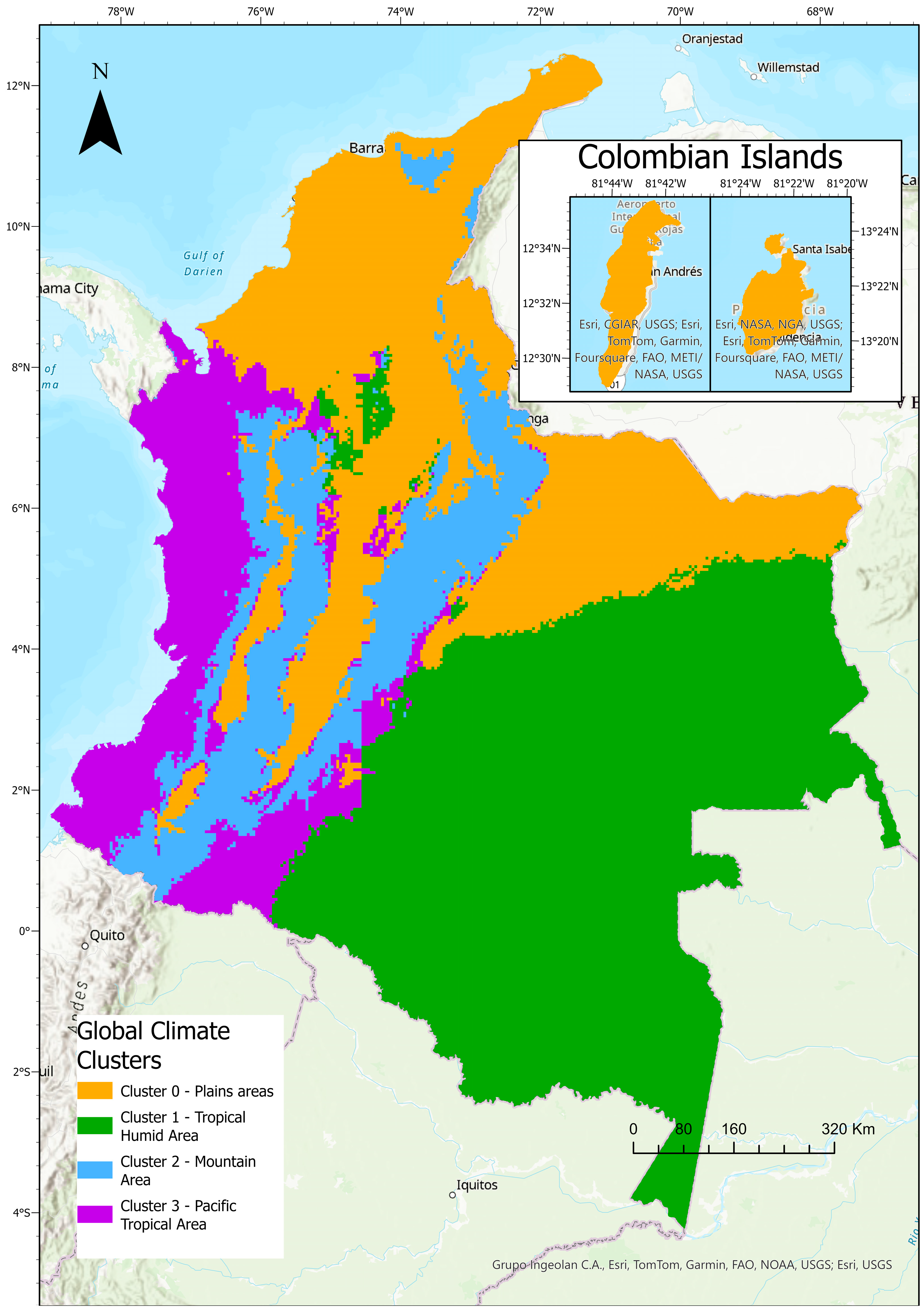
4.1. Global Analysis and Clustering Process
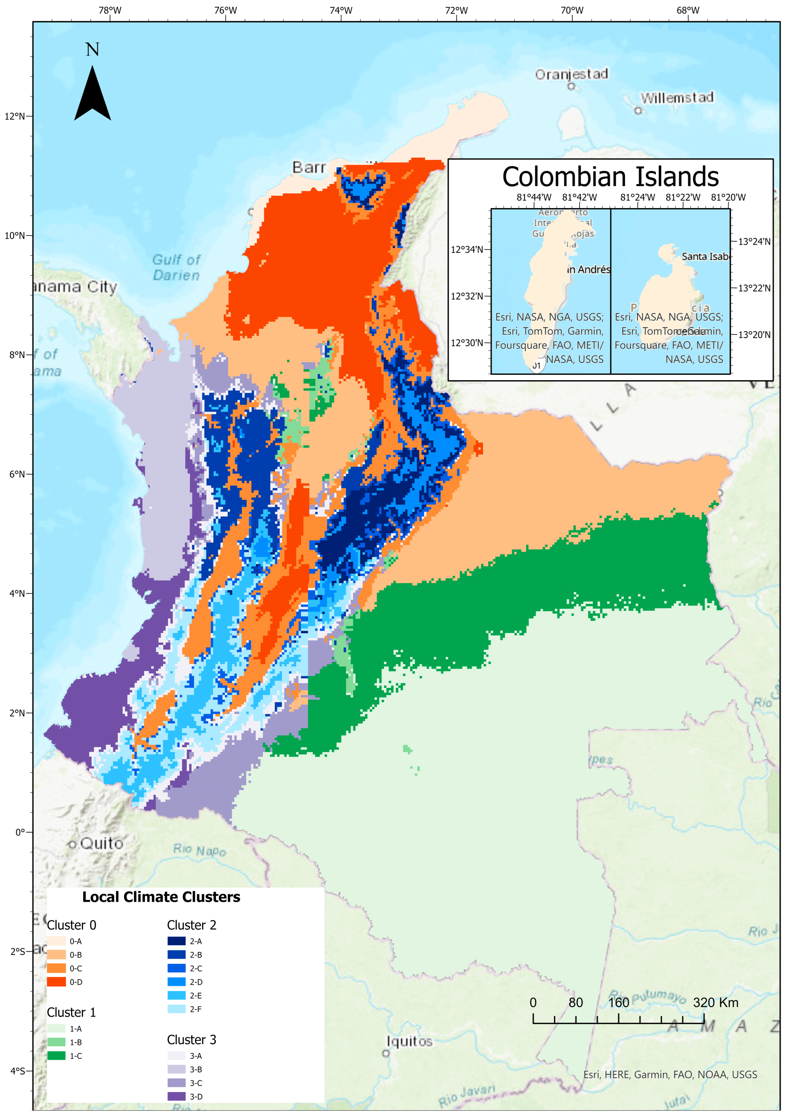
4.2. Microclimate Configuration
5. Discussion
5.1. Key Research Findings
5.2. Contributions toward Practice
6. Conclusions
Author Contributions
Funding
Institutional Review Board Statement
Informed Consent Statement
Data Availability Statement
Acknowledgments
Conflicts of Interest
References
- Perera, N.G.R.; Emmanuel, R. A “Local Climate Zone” Based Approach to Urban Planning in Colombo, Sri Lanka. Urban. Clim. 2018, 23, 188–203. [Google Scholar] [CrossRef]
- Reckien, D.; Salvia, M.; Heidrich, O.; Church, J.M.; Pietrapertosa, F.; De Gregorio-Hurtado, S.; D’Alonzo, V.; Foley, A.; Simoes, S.G.; Krkoška Lorencová, E.; et al. How Are Cities Planning to Respond to Climate Change? Assessment of Local Climate Plans from 885 Cities in the EU-28. J. Clean. Prod. 2018, 191, 207–219. [Google Scholar] [CrossRef]
- Davidson, A.S.; Malet-Damour, B.; Praene, J.P. A New Microclimate Zoning Method Based on Multivariate Statistics: The Case of Reunion Island. Urban. Clim. 2023, 52, 101687. [Google Scholar] [CrossRef]
- Mejía-Parada, C.; Mora-Ruiz, V.; Attia, S. Bioclimatic Design Recommendations for Novel Cluster Analysis-Based Mapping for Humid Climates with Altitudinal Gradient Variations. J. Build. Eng. 2024, 82, 108262. [Google Scholar] [CrossRef]
- Ascencio-Vásquez, J.; Brecl, K.; Topič, M. Methodology of Köppen-Geiger-Photovoltaic Climate Classification and Implications to Worldwide Mapping of PV System Performance. Sol. Energy 2019, 191, 672–685. [Google Scholar] [CrossRef]
- Attia, S.; Lacombe, T. Architect-Friendly Climate Analysis Tool for Bioclimatic Design in Hot Humid Climates. In Proceedings of the Building Simulation 2019: 16th Conference of International Building Performance Simulation Association, Rome, Italy, 2–4 September 2019; Volume 7, pp. 4785–4792. [Google Scholar]
- Sengupta, M.; Xie, Y.; Lopez, A.; Habte, A.; Maclaurin, G.; Shelby, J. The National Solar Radiation Data Base (NSRDB). Renew. Sustain. Energy Rev. 2018, 89, 51–60. [Google Scholar] [CrossRef]
- Nguyen, P.; Ombadi, M.; Gorooh, V.A.; Shearer, E.J.; Sadeghi, M.; Sorooshian, S.; Hsu, K.; Bolvin, D.; Ralph, M.F. Persiann Dynamic Infrared–Rain Rate (PDIR-Now): A near-Real-Time, Quasi-Global Satellite Precipitation Dataset. J. Hydrometeorol. 2020, 21, 2893–2906. [Google Scholar] [CrossRef] [PubMed]
- Walsh, A.; Cóstola, D.; Labaki, L.C. Review of Methods for Climatic Zoning for Building Energy Efficiency Programs. Build. Environ. 2017, 112, 337–350. [Google Scholar] [CrossRef]
- Peel, M.C.; Finlayson, B.L.; McMahon, T.A. Updated World Map of the Köppen-Geiger Climate Classification. Hydrol. Earth Syst. Sci. 2007, 11, 1633–1644. [Google Scholar] [CrossRef]
- Beck, H.E.; Zimmermann, N.E.; McVicar, T.R.; Vergopolan, N.; Berg, A.; Wood, E.F. Present and Future Köppen-Geiger Climate Classification Maps at 1-Km Resolution. Sci. Data 2018, 5, 180214. [Google Scholar] [CrossRef]
- Martinopoulos, G.; Alexandru, A.; Papakostas, K.T. Mapping Temperature Variation and Degree-Days in Metropolitan Areas with Publicly Available Sensors. Urban. Clim. 2019, 28, 100464. [Google Scholar] [CrossRef]
- Omarov, B.; Memon, S.A.; Kim, J. A Novel Approach to Develop Climate Classification Based on Degree Days and Building Energy Performance. Energy 2023, 267, 126514. [Google Scholar] [CrossRef]
- Roshan, G.; Farrokhzad, M.; Attia, S. Climatic Clustering Analysis for Novel Atlas Mapping and Bioclimatic Design Recommendations. Indoor Built Environ. 2021, 30, 313–333. [Google Scholar] [CrossRef]
- Manzano-Agugliaro, F.; Montoya, F.G.; Sabio-Ortega, A.; García-Cruz, A. Review of Bioclimatic Architecture Strategies for Achieving Thermal Comfort. Renew. Sustain. Energy Rev. 2015, 49, 736–755. [Google Scholar] [CrossRef]
- Liu, S.; Shi, Q. Local Climate Zone Mapping as Remote Sensing Scene Classification Using Deep Learning: A Case Study of Metropolitan China. ISPRS J. Photogramm. Remote Sens. 2020, 164, 229–242. [Google Scholar] [CrossRef]
- Kotharkar, R.; Bagade, A. Local Climate Zone Classification for Indian Cities: A Case Study of Nagpur. Urban. Clim. 2018, 24, 369–392. [Google Scholar] [CrossRef]
- Wicki, A.; Parlow, E. Attribution of Local Climate Zones Using a Multitemporal Land Use/Land Cover Classification Scheme. J. Appl. Remote Sens. 2017, 11, 026001. [Google Scholar] [CrossRef]
- Nadarajah, P.D.; Singh, M.K.; Mahapatra, S.; Pajek, L.; Košir, M. Bioclimatic Classification for Building Energy Efficiency Using Hierarchical Clustering: A Case Study for Sri Lanka. J. Build. Eng. 2023, 83, 108388. [Google Scholar] [CrossRef]
- Praene, J.-P.; Malet-Damour, B.; Harimisa Radanielina, M.; Fontaine, L.; Riviere, G.; Philippe Praene, J.; Rivière, G. GIS-Based Approach to Identify Climatic Zoning: A Hierarchical Clustering on Principal Component Analysis GIS-Based Approach to Define Climatic Zoning: A Hierarchical Clustering on Principal Component Analysis. Build. Environ. 2019, 164, 106330. [Google Scholar] [CrossRef]
- Zscheischler, J.; Mahecha, M.D.; Harmeling, S. Climate Classifications: The Value of Unsupervised Clustering. Procedia Comput. Sci. 2012, 9, 897–906. [Google Scholar] [CrossRef]
- Li, T.; Rezaeipanah, A.; Tag El Din, E.S.M. An Ensemble Agglomerative Hierarchical Clustering Algorithm Based on Clusters Clustering Technique and the Novel Similarity Measurement. J. King Saud. Univ. Comput. Inf. Sci. 2022, 34, 3828–3842. [Google Scholar] [CrossRef]
- Bienvenido-Huertas, D.; Marín-García, D.; Carretero-Ayuso, M.J.; Rodríguez-Jiménez, C.E. Climate Classification for New and Restored Buildings in Andalusia: Analysing the Current Regulation and a New Approach Based on k-Means. J. Build. Eng. 2021, 43, 102829. [Google Scholar] [CrossRef]
- Sinaga, K.P.; Yang, M.S. Unsupervised K-Means Clustering Algorithm. IEEE Access 2020, 8, 80716–80727. [Google Scholar] [CrossRef]
- Bradley, P.S.; Fayyad, U.M. Refining Initial Points for K-Means Clustering. ICML 1998, 98, 91–99. [Google Scholar]
- Yuan, C.; Yang, H. Research on K-Value Selection Method of K-Means Clustering Algorithm. J 2019, 2, 226–235. [Google Scholar] [CrossRef]
- Bechtel, B.; Daneke, C. Classification of Local Climate Zones Based on Multiple Earth Observation Data. IEEE J. Sel. Top. Appl. Earth Obs. Remote Sens. 2012, 5, 1191–1202. [Google Scholar] [CrossRef]
- Grupo de Climatología y Agrometeoreología-Subdirección de Metereología, IDEAM. Clasificaciones Climaticas Colombia. In Proceedings of the Segundo Congreso Nacional del Clima, Bogotá, Colombia, 3–5 August 2011. [Google Scholar]
- IDEAM. Evolución Del Índice de Confort Térmico Por Periodos 1971–2000. Segunda Comunicación Nacional ante la Convención Marco de las Naciones Unidad sobre Cambio Climático; Instituto de Hidrología, Meteorología y Estudios Ambientales—IDEAM: Bogotá, Colombia, 2010.
- Ministerio de Ambiente y Desarrollo Sostenible. Criterios Ambientales Para El Diseño y Construccion de Vivienda Urbana; Ministerio de Ambiente y Desarrollo Sostenible: Bogotá, Colombia, 2012; ISBN 9789588491585.
- Gillies, S. Rasterio Documentat, 23rd ed.; MapBox: San Francisco, CA, USA, 2019. [Google Scholar]
- Brimicombe, C.; Di Napoli, C.; Quintino, T.; Pappenberger, F.; Cornforth, R.; Cloke, H.L. Thermofeel: A Python Thermal Comfort Indices Library. SoftwareX 2022, 18, 101005. [Google Scholar] [CrossRef]
- Li, H.; Huang, J.; Hu, Y.; Wang, S.; Liu, J.; Yang, L. A New TMY Generation Method Based on the Entropy-Based TOPSIS Theory for Different Climatic Zones in China. Energy 2021, 231, 120723. [Google Scholar] [CrossRef]
- Tadić, L.; Bonacci, O.; Brleković, T. An Example of Principal Component Analysis Application on Climate Change Assessment. Theor. Appl. Climatol. 2019, 138, 1049–1062. [Google Scholar] [CrossRef]
- Jollife, I.T.; Cadima, J. Principal Component Analysis: A Review and Recent Developments. Philos. Trans. R. Soc. A Math. Phys. Eng. Sci. 2016, 374, 20150202. [Google Scholar] [CrossRef]
- Kaiser, H.F. The Application of Electronic Computers to Factor Analysis. Educ. Psychol. Meas. 1960, 20, 141–151. [Google Scholar] [CrossRef]
- Xiong, J.; Yao, R.; Grimmond, S.; Zhang, Q.; Li, B. A Hierarchical Climatic Zoning Method for Energy Efficient Building Design Applied in the Region with Diverse Climate Characteristics. Energy Build. 2019, 186, 355–367. [Google Scholar] [CrossRef]
- Dinh, D.T.; Fujinami, T.; Huynh, V.N. Estimating the Optimal Number of Clusters in Categorical Data Clustering by Silhouette Coefficient. In Knowledge and Systems Sciences. KSS 2019; Communications in Computer and Information Science; Springer: Singapore, 2019; Volume 1103, pp. 1–17. [Google Scholar]
- Brusco, M.J.; Steinley, D. A Comparison of Heuristic Procedures for Minimum Within-Cluster Sums of Squares Partitioning. Psychometrika 2007, 72, 583–600. [Google Scholar] [CrossRef]
- Semahi, S.; Benbouras, M.A.; Mahar, W.A.; Zemmouri, N.; Attia, S. Development of Spatial Distribution Maps for Energy Demand and Thermal Comfort Estimation in Algeria. Sustainability 2020, 12, 6066. [Google Scholar] [CrossRef]
- Gupta, R.; Mathur, J.; Garg, V. Assessment of Climate Classification Methodologies Used in Building Energy Efficiency Sector. Energy Build. 2023, 298, 113549. [Google Scholar] [CrossRef]
- Oliveira, A.; Lopes, A.; Niza, S. Local Climate Zones in Five Southern European Cities: An Improved GIS-Based Classification Method Based on Copernicus Data. Urban. Clim. 2020, 33, 100631. [Google Scholar] [CrossRef]
- Bechtel, B.; Alexander, P.J.; Böhner, J.; Ching, J.; Conrad, O.; Feddema, J.; Mills, G.; See, L.; Stewart, I. Mapping Local Climate Zones for a Worldwide Database of the Form and Function of Cities. ISPRS Int. J. Geoinf. 2015, 4, 199–219. [Google Scholar] [CrossRef]
- Abbasi, F.; Bazgeer, S.; Kalehbasti, P.R.; Oskoue, E.A.; Haghighat, M.; Kalehbasti, P.R. New Climatic Zones in Iran: A Comparative Study of Different Empirical Methods and Clustering Technique. Theor. Appl. Climatol. 2022, 147, 47–61. [Google Scholar] [CrossRef]
- Sathiaraj, D.; Huang, X.; Chen, J. Predicting Climate Types for the Continental United States Using Unsupervised Clustering Techniques. Environmetrics 2019, 30, e2524. [Google Scholar] [CrossRef]
- Balogun, I.A.; Daramola, M.T. The Outdoor Thermal Comfort Assessment of Different Urban Configurations within Akure City, Nigeria. Urban. Clim. 2019, 29, 100489. [Google Scholar] [CrossRef]
- Attia, S.; Lacombe, T.; Rakotondramiarana, H.T.; Garde, F.; Roshan, G.R. Analysis Tool for Bioclimatic Design Strategies in Hot Humid Climates. Sustain. Cities Soc. 2019, 45, 8–24. [Google Scholar] [CrossRef]
- Daemei, A.B.; Eghbali, S.R.; Khotbehsara, E.M. Bioclimatic Design Strategies: A Guideline to Enhance Human Thermal Comfort in Cfa Climate Zones. J. Build. Eng. 2019, 25, 100758. [Google Scholar] [CrossRef]
- Li, Z.; Feng, X.; Fan, X.; Sun, J.; Fang, Z. Effect of Direct Solar Projected Area Factor on Outdoor Thermal Comfort Evaluation: A Case Study in Shanghai, China. Urban. Clim. 2022, 41, 101033. [Google Scholar] [CrossRef]
- Anderson, R.; Bayer, P.E.; Edwards, D. Climate Change and the Need for Agricultural Adaptation. Curr. Opin. Plant Biol. 2020, 56, 197–202. [Google Scholar] [CrossRef] [PubMed]
- Kogo, B.K.; Kumar, L.; Koech, R. Climate Change and Variability in Kenya: A Review of Impacts on Agriculture and Food Security. Environ. Dev. Sustain. 2021, 23, 23–43. [Google Scholar] [CrossRef]
- Attia, S.; Eleftheriou, P.; Xeni, F.; Morlot, R.; Ménézo, C.; Kostopoulos, V.; Betsi, M.; Kalaitzoglou, I.; Pagliano, L.; Cellura, M.; et al. Overview and Future Challenges of Nearly Zero Energy Buildings (NZEB) Design in Southern Europe. Energy Build. 2017, 155, 439–458. [Google Scholar] [CrossRef]
- Santos-Herrero, J.M.; Lopez-Guede, J.M.; Flores-Abascal, I. Modeling, Simulation and Control Tools for NZEB: A State-of-the-Art Review. Renew. Sustain. Energy Rev. 2021, 142, 110851. [Google Scholar] [CrossRef]
- Belussi, L.; Barozzi, B.; Bellazzi, A.; Danza, L.; Devitofrancesco, A.; Fanciulli, C.; Ghellere, M.; Guazzi, G.; Meroni, I.; Salamone, F.; et al. A Review of Performance of Zero Energy Buildings and Energy Efficiency Solutions. J. Build. Eng. 2019, 25, 100772. [Google Scholar] [CrossRef]
- Dnp Colombia, Potencial Mundial De La Vida. Bases Del Plan Nacional de Desarrollo 2022–2026; Departamento Nacional de Planeación: Bogotá, Colombia, 2022.


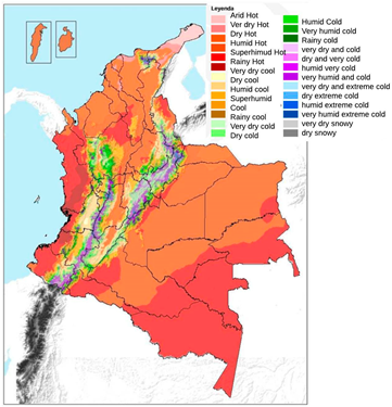
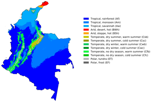 Köppen–Geiger Classification [11] | 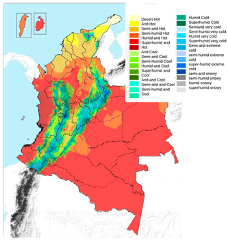 Caldas–Lang Classification [28] |
| Use: climatology, agriculture, geography, hydrology. | Use: agriculture, climatology, biodiversity. |
 Holdridge Classification [28] | 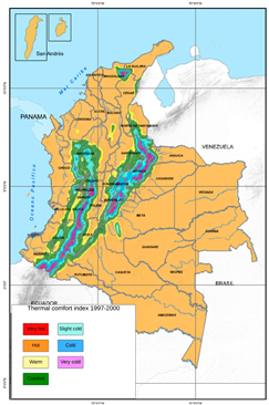 Thermal Comfort Classification [29] |
| Use: agriculture, ecology, biology, land-use planning. | Use: thermal comfort evaluation. |
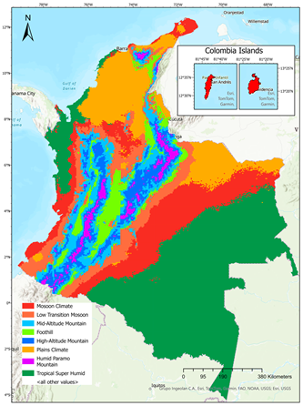 Bioclimatic design zoning [4] |  Climate Zoning [30] |
| Use: architecture and building design. | Use: architecture and building recommendations. |
| Global Cluster | Max. Temperature (°C) | Max. Relative Humidity (%) | Min. Temperature (°C) | Min. Relative Humidity (%) | Mean Wind Speed (m/s) | Daily Cumulative GHI (w/m2) | Cumulative Rainfall Mean (mm) | Elevation (m) | |
|---|---|---|---|---|---|---|---|---|---|
| Cluster 0 | Average | 31.13 | 90.91 | 22.91 | 54.90 | 1.11 | 5385.29 | 5.77 | 330.07 |
| Min. | 20.82 | 65.15 | 12.22 | 35.66 | 0.02 | 3614.93 | 0.83 | 0.00 | |
| Max. | 36.85 | 100.00 | 28.24 | 81.34 | 7.61 | 6531.18 | 12.55 | 2600 | |
| Std | 2.41 | 6.45 | 2.29 | 8.02 | 1.14 | 348.03 | 2.08 | 416.24 | |
| Cluster 1 | Average | 28.29 | 99.76 | 22.51 | 76.59 | 0.26 | 4851.96 | 9.02 | 209.29 |
| Min. | 23.04 | 94.14 | 15.03 | 58.02 | 0.05 | 4183.88 | 5.52 | 40 | |
| Max. | 30.89 | 100.00 | 24.24 | 89.27 | 1.68 | 5585.80 | 11.32 | 1555 | |
| Std | 0.68 | 0.58 | 0.58 | 4.23 | 0.33 | 144.51 | 1.06 | 116.61 | |
| Cluster 2 | Average | 18.76 | 99.36 | 10.74 | 74.12 | 1.11 | 4410.98 | 4.77 | 2442.84 |
| Min. | 3.40 | 81.23 | −4.76 | 50.3 | 0.03 | 2688.17 | 1.75 | 773 | |
| Max. | 26.73 | 100.00 | 19.44 | 100.00 | 3.69 | 6227.63 | 11.89 | 5081 | |
| Std | 3.91 | 2.00 | 4.05 | 11.35 | 0.49 | 654.43 | 1.67 | 693.47 | |
| Cluster 3 | Average | 27.92 | 95.32 | 21.92 | 68.21 | 1.00 | 4304.76 | 11.31 | 440.47 |
| Min. | 20.93 | 73.61 | 13.99 | 45.12 | 0.03 | 2894.31 | 3.45 | 3.00 | |
| Max. | 31.69 | 100.00 | 27.41 | 97.9 | 3.94 | 5555.64 | 24.4 | 2118 | |
| Std | 1.72 | 4.63 | 2.42 | 9.24 | 0.85 | 421.83 | 3.77 | 443.85 | |
| Climate Conditions | Global Cluster 0 |
|---|---|
| Max. Temperature | 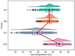 |
| Max. Relative Humidity | 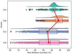 |
| Min. Temperature | 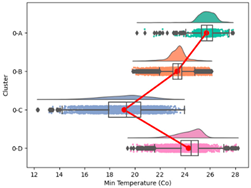 |
| Min. Relative Humidity |  |
| Mean Wind Speed | 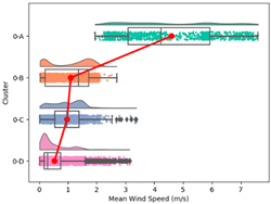 |
| Daily Cumulative GHI | 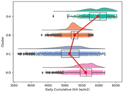 |
| Cumulative Daily Rainfall | 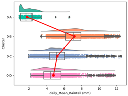 |
| Elevation |  |
| Climate Conditions | Global Cluster 1 |
|---|---|
| Max. Temperature |  |
| Max. Relative Humidity | 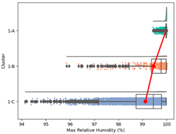 |
| Min. Temperature | 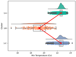 |
| Min. Relative Humidity | 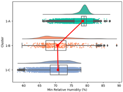 |
| Mean Wind Speed | 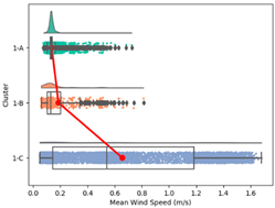 |
| Daily Cumulative GHI |  |
| Cumulative Daily Rainfall | 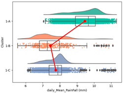 |
| Elevation | 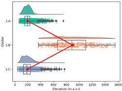 |
| Climate Conditions | Global Cluster 2 |
|---|---|
| Max. Temperature |  |
| Max. Relative Humidity |  |
| Min. Temperature | 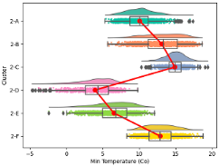 |
| Min. Relative Humidity |  |
| Mean Wind Speed |  |
| Daily Cumulative GHI |  |
| Cumulative Daily Rainfall |  |
| Elevation |  |
| Climate Conditions | Global Cluster 3 |
|---|---|
| Max. Temperature |  |
| Max. Relative Humidity |  |
| Min. Temperature |  |
| Min. Relative Humidity |  |
| Mean Wind Speed |  |
| Daily Cumulative GHI |  |
| Cumulative Daily Rainfall |  |
| Elevation |  |
Disclaimer/Publisher’s Note: The statements, opinions and data contained in all publications are solely those of the individual author(s) and contributor(s) and not of MDPI and/or the editor(s). MDPI and/or the editor(s) disclaim responsibility for any injury to people or property resulting from any ideas, methods, instructions or products referred to in the content. |
© 2024 by the authors. Licensee MDPI, Basel, Switzerland. This article is an open access article distributed under the terms and conditions of the Creative Commons Attribution (CC BY) license (https://creativecommons.org/licenses/by/4.0/).
Share and Cite
Mejía-Parada, C.; Mora-Ruiz, V.; Soto-Paz, J.; Parra-Orobio, B.A.; Attia, S. Microclimate Zoning Based on Double Clustering Method for Humid Climates with Altitudinal Gradient Variations: A Case Study of Colombia. Atmosphere 2024, 15, 709. https://doi.org/10.3390/atmos15060709
Mejía-Parada C, Mora-Ruiz V, Soto-Paz J, Parra-Orobio BA, Attia S. Microclimate Zoning Based on Double Clustering Method for Humid Climates with Altitudinal Gradient Variations: A Case Study of Colombia. Atmosphere. 2024; 15(6):709. https://doi.org/10.3390/atmos15060709
Chicago/Turabian StyleMejía-Parada, Cristian, Viviana Mora-Ruiz, Jonathan Soto-Paz, Brayan A. Parra-Orobio, and Shady Attia. 2024. "Microclimate Zoning Based on Double Clustering Method for Humid Climates with Altitudinal Gradient Variations: A Case Study of Colombia" Atmosphere 15, no. 6: 709. https://doi.org/10.3390/atmos15060709