Abstract
Quality control (QC) of HaiYang-2B (HY-2B) satellite data is mainly based on the observation process, which remains uncertain for data assimilation (DA). The data in operation have not been widely used in numerical weather prediction. To ensure HY-2B data meet the theoretical assumptions for DA applications, the iterated reweighted minimum covariance determinant (IRMCD) QC method was studied in HY-2B data based on the typhoon “Chanba”. The statistical results showed that most of the outliers were eliminated, and the observation increment distribution of the HY-2B data after QC (QCed) was closer to a Gaussian distribution than the raw data. The kurtosis and skewness of the QCed data were much closer to zero. The QCed track demonstrated the lowest accumulated error and the best intensity in typhoon assimilation, and the QCed intensity was closest to the observation during the nearshore enhancement, exhibiting the strongest intensity among the experiment. Further analysis revealed that the improvement was accompanied by a significant reduction in vertical wind shear during the nearshore enhancement of the typhoon. The QCed moisture flux divergence and vertical velocity in the upper layer increased significantly, which promoted the upward transport of momentum in the lower layers and contributed to the maintenance of the typhoon’s barotropic structure. Compared with the assimilation of raw data, the effective removal of outliers using the IRMCD algorithm significantly improved the simulation results for typhoons.
1. Introduction
Observational data are essential for the assimilation of numerical weather predictions (NWP); however, the acquisition of ocean surface wind (OWS) field data is challenging because of limited observation equipment. Satellite-borne scatterometers are effective in observing wind over the ocean [1,2,3,4,5]. The launch of the HaiYang-2B (HY-2B) satellite equipped with a Ku-band scatterometer (HSCAT-B) improved the capacity to acquire OWS data and is expected to further improve NWP. However, because the satellite was launched recently, the data are still relatively new, and a large amount of high-precision satellite data implies more intensive information, which requires further utilization and research.
As with that of previous scatterometers, the data quality of HSCAT-B is associated with the complex principle of microwave scattering making the sensitivity of the radar cross section (σ_0) to sea surface roughness change with wind velocity. At the same time, rainfall causes backscattering attenuation, which affects data accuracy [6,7,8]. Nevertheless, HY-2B data have demonstrated superior quality compared to that of other products in its class [9,10,11] and have been utilized in various applications. In some studies on data applications, HSCAT-B data have shown good application value. Applying HSCAT-B data to the GRAPES 4DVar system affected the analysis of wind, geopotential height, and temperature extending from the boundary layer to the troposphere [12]. An enhancement in forecasting skill was achieved, indicating the effectiveness of the HY-2B data for NWP. HY-2B scatterometer data have also been applied to typhoon location and characterization intensity in some studies, showing that the radial extent of 17 m/s winds can well characterize the cyclone intensity and actual path [13,14].
However, HY-2B data have not been widely used for assimilation in NWP because the observations are not completely accurate and contain different errors, such as instrumental and representative errors [15], which cannot be directly applied in assimilation systems. To improve the utilization of satellite data, equitable data filtering and quality control (QC) for data assimilation (DA) applications are required. Nevertheless, the forecasting results cannot be improved if only traditional algorithms are used. To identify and eliminate obvious outliers from observation data, some traditional algorithms such as range and extreme value checks are commonly used in QC. Based on meteorological experience and statistical methods, thresholds are defined to identify data outside the threshold as outliers [16,17,18,19,20]. However, conventional judgment methods are relatively simplistic, inflexible, and unsuitable for the analysis of complex data and can easily misjudge normal extreme values as outliers. Moreover, statistical measures such as the mean and standard deviation in QC are often used for error evaluation; however, outliers with large deviations can also affect the mean and standard deviation of the dataset, resulting in the misjudgment of outliers. Nevertheless, conventional methods for observing products are performed without considering their association with the model background field. Using HY-2B data as an example, a QC method was developed based on the singularity exponent, which demonstrated good performance in an ASCAT satellite [21,22]. However, QC focuses only on removing outliers and revising the optimal solution during the inversion process, resulting in an uncertain impact of observation data in assimilation applications.
Biweight standard derivation (BSD) is an effective algorithm for reducing the influence of outliers on the mean and standard deviation [23]. In some studies, the BSD method is used as a single variable, which has been applied in many studies, such as wind profiler observations, to compare methods for estimating the uncertainty in the temperature of meteorological stations and identify cloud radiation [15,24,25,26]. For multivariable or multidimensional data, such as wind velocity (u/v), the minimum covariance determinant (MCD) approach is more appropriate, which is one of the affine-equivariant and highly robust multivariate outlier detection rules [27,28,29]. After the fast-MCD algorithm was proposed based on MCD, the computational efficiency improved [30,31], and the algorithm has since then been widely used in many fields. To reduce the misjudgment of outliers, Cerioli proposed an iterated reweighted minimum covariance determinant (IRMCD) method based on the MCD method [32], which has proven to be effective in the meteorological field [26,27,32]. In the current study, the IRMCD algorithm was mainly used for the QC of wind profile observations; however, for HY-2B data, especially for scatterometer observations, limited research has been conducted.
To explore the QC of HY-2B data toward the assimilation application of the IRMCD method, we incorporated the model background field and processed the observation increment (OMB). The typhoon “Chanba” was taken as an example to explore the influence of application and forecasting using HSCAT-B L2B level products in DA with IRMCD. This study is divided into six sections. In Section 2, the IRMCD method is introduced. The data and physical parameterization scheme in the numerical model are presented in Section 3. In Section 4, the results of the experiment, including the statistical and case study results, are presented. Section 5 presents an analysis of further research, and a summary and discussion are presented in Section 6.
2. IRMCD
An observation dataset of n vector with dimensions can be set as follows:
The th vector is represented by . The mean vector and covariance matrix of the dataset are represented by and , respectively.
The existence of outliers in the dataset indicates that the data have been contaminated (including and ). In the statistical analysis, the value in with a large distance difference from the distribution is defined as an outlier by calculating the square of the robust distance in each sample, where the nominal size is commonly accepted.
IRMCD is a highly robust estimation method based on the reweighted MCD estimator [32]. The steps in the IRMCD method for finite sample outlier detection are as follows.
Step 1. In sample , observations are taken to iterate the whole sample, and k observations with the smallest determinant of covariance matrix are selected as the subset of MCD. The maximum possible breakdown point can be taken as with the integer part of , . Another choice is .
The mean of the MCD subset is given as follows:
and the covariance is given as follows:
C is a proportional constant, making both consistent and unbiased [32].
Step 2. Define the square of the robust distance of the sample:
where represents the distance between each observation point and the location of the data center.
Step 3. To improve efficiency, data need to be reweighted (RMCD), where the mean vector () and covariance matrix () are given as follows:
and
the threshold of is recommended to be 0.975 with distribution of and the outlier detection problem is usually phrased in terms of testing the n null hypothesis; if it satisfies , the observation is good [32]. The weight of each observation was determined using .
The new reweighted robust distance changes to the following:
Step 4. After considering the different situations of the weights above, the specific form of the reweighted distance (FSRMCD) is obtained:
where is the distribution function of Beta, and are the shape parameters.
Step 5. Furthermore, to correct the problem of different elimination effects caused by different and , the iterative process (IRMCD) of the multiple outlier test is added.
The is the quantile consistent with the Beta distribution in (10), where is the threshold. If condition (11) holds, the sample is considered to accept , which is a non-outlier value; otherwise, it is considered an outlier.
3. Data and Experiment
3.1. Data
In this study, the background field used comes from the fifth generation of the ECMWF global climate reanalysis (ERA5) with a time resolution of 3 h and grid resolution of , which is one of the best-quality data sources in operational applications. The analysis of the meteorological element field in Section 5 was also compared with the ERA5 data: “https://cds.climate.copernicus.eu/cdsapp#!/search?type=dataset (accessed on 11 April 2023)”.
The typhoon track and intensity data were obtained from the International Climate Management Best Tracks (IBTrACS). The best track data were obtained from all available Regional Specialized Meteorological Centers (RSMCs) and other agencies, and the statistical data were summarized by various agencies “https://www.ncei.noaa.gov/products/international-best-track-archive (accessed on 20 August 2022)”.
The observation data used for assimilation were obtained from the National Satellite Ocean Application Center HY-2B scatterometer L2B level data source, mainly for the observation of the sea surface wind field. The backscattering coefficient was derived from the NSCAT-4 geophysical model function, and the wind filed was from the numerical weather forecast and HY-2B satellite microwave scatterometer [33,34]. The wind retrieval method based on the multiple solution combination (MSC) and 2DVAR ensures data quality. The resolution of the wind cell was 25 km × 25 km, and the sampling time was from 00:00 on 30 June 2022 to 00:00 on 3 July 2022: “https://osdds.nsoas.org.cn/MarineDynamic (accessed on 19 April 2023)”.
3.2. Numerical Prediction Model and Assimilation System
The WRFv4.0 (ARW) model was used for numerical simulation in this study. The grid resolution was set to , and the area was (Figure 1), which is mainly concentrated in the South China Sea area, covering Guangdong Province. The experimental period was from 30 June to 3 July 2022, starting at 12 UTC, with a forecast time limit of 48 h. The specific parameterization scheme and experimental settings are as presented in Table 1.
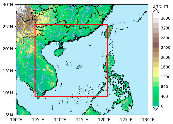
Figure 1.
Terrain height; red rectangular box is forecasting experiment area (South China Sea).

Table 1.
Parameterization schemes for physical processes set in WRF.
In this study, a Gridpoint Statistical Interpolation (GSI) assimilation system was used to interpolate and assimilate the observational data to obtain an analysis field as a new initial field for the next time step. The assimilation scheme was 3DVAR with the assimilation time of 30 June 2022, at 12 UTC, and the assimilation window of observation was ±1.5 h. In the assimilation scheme, the CTRL experiment did not use the observational data. EXP-HY2B assimilated only HY-2B and did not undergo the QC. The EXP-IRMCD assimilated HY-2B data and proceeded with the QC (Table 2). The region of DA was consistent with that of the simulation ().
Table 2.
The scheme of assimilation experiment.
3.3. Quality Control Routine
The quality control of this experiment was divided into two parts: statistical QC analysis and case study QC experiments (Figure 2). The statistical QC provided a Gaussian distribution theoretical assumption for the assimilation experiment of cases, ensuring that the QC method was effective on HY2B data and conformed to the theoretical basis of assimilation; the case experiment verified the specific effects of the IRMCD method on short-term forecasts. The specific steps are as follows:
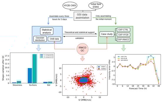
Figure 2.
Data assimilation experiment framework.
Statistical Analysis: The HY2B data from 30 June at 00 UTC to 3 July at 00 UTC covered the entire typhoon process.
1. The HY2B data were assimilated every three hours, and the satellite data were divided with a time window of ±1.5 h, for the temporal resolution is much higher than the assimilation time interval. Data affected by land were eliminated by the quality flag in the dataset.
2. The ERA5 data consistent with the observation time had an interval of three hours. The data at each time were preprocessed to serve as the background field for assimilation.
3. Since the GSI assimilation could only assimilate one moment at a time, this study wrote a batch operation program for WRF and GSI to perform cycle assimilation at each moment.
4. The QC object of this paper was OMB data. For every analysis field generated in GSI, a diagnostic file containing background and observational information was attached. The diagnostic tools built into the GSI system could extract the OMB information from the file. Finally, the OMB data of each moment was integrated, and the missing measurement information was removed, resulting in a total sample size of 34,429.
5. Using IRMCD methods, we could identify inliers and outliers, and subsequently perform statistical analysis on both groups.
Case study: 1. The EXP-CTRL did not analyze any data and performed a routine 48 h simulation.
2. The EXP-HY2B only considered the information at the initial moment, using the analysis field at 12 UTC on 30 June as the initial condition for a 48 h forecast.
3. The EXP-HY2B was consistent with the EXP-HY2B, but observations judged to be outliers in the OMB were removed. The inliers were re-assimilated to generate a new analysis field and then forecast.
4. Results
4.1. Statistical Results
To explore the statistical results of the IRMCD method, this study obtained 3 days of wind OMB data (covering the process from typhoon generation to landing) from 30 June 2022 at 00 UTC to 3 July 2022 at 00 UTC. Due to the GSI system not being able to directly extract the background field, the background information in Figure 3 was obtained by subtracting OMB from the observations. Additionally, in Figure 5, to determine whether the OMB was close to Gaussian distribution, the ideal Gaussian distribution (y-axis) was fitted from the mean and standard deviation of the OMB. Therefore, the closer the OMB distribution was to the theoretical Gaussian distribution, the more the data distribution approached a straight line.
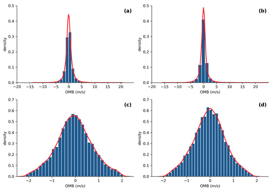
Figure 3.
Probability density distribution of the observation increment (OMB), u-wind (left), and v-wind (right) during 30 June, 00 UTC–3 July, 00 UTC 2022; before QC (a,b); after QC (c,d).
As shown in Figure 3, the Gaussian distribution of the u/v component was not evident before QC, and large outliers were distributed at both ends of the data. Most large observation increments in the processed data were eliminated, the center density values of the distribution increased, and the entire distribution was more concentrated in the middle. The quantile–quantile (Q–Q) scatterplots (Figure 4) converge to a straight line, proving that the elimination effect was significant. Figure 5 shows that scatter points with a large difference from the background field were eliminated, and the scatter was more densely distributed on the diagonal.
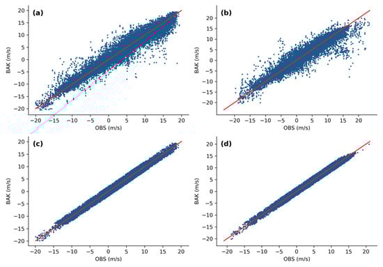
Figure 4.
Distribution of observation (x-axis) and background filed (y-axis); u-wind (left), v-wind (right) during 30 June, 00 UTC−3 July, 00 UTC 2022; before QC (a,b); after QC (c,d).
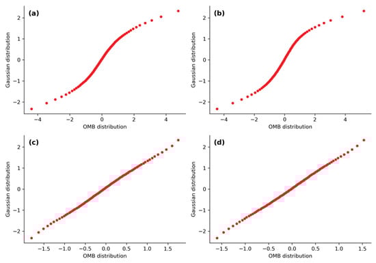
Figure 5.
Quantile–quantile (Q–Q) scatterplots; u-wind (left), and v-wind (right) during 30 June, 00 UTC−3 July, 00 UTC 2022; before QC (a,b); after QC (c,d).
Table 3 lists the kurtosis, skewness, and standard deviation values before and after QC. The closer the kurtosis and skewness values were to zero, the more the data distribution conformed to a Gaussian distribution. The data were more biased toward the middle after QC, and the effect of kurtosis of the u/v component was the most obvious, indicating that there were more outliers in the tail of the data. After data processing, kurtosis decreased from 9.491/18.341 to −0.106/−0.156, resulting in a flatter distribution. In addition, regardless of skewness or kurtosis, the values of the v component were more than twice those of the u component, and its outliers were generally higher than those of the u component, indicating that the v component was the main component causing data pollution.
Table 3.
Skewness and kurtosis of OMB data with u/v component before and after application of QC.
4.2. Wind Fields and Analysis Increment
The wind field of the HY-2B data at the assimilation time is shown in Figure 6, where the red barbs represent the data that were removed by the IRMCD method, that is, the wind speed that differs significantly from the background field. The outliers determined by this algorithm are mainly distributed south of the typhoon center and near the eye. This indicates that the observation of HY-2B data at the tropical cyclone center is not beneficial for the prediction of the model during assimilation.
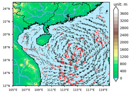
Figure 6.
Wind field of observation on 30 June, 12 UTC 2022; the red barbs are the outliers based on the IRMCD.
The analysis increment was defined as the meteorological element field after assimilation minus the pre-assimilation field, which was intended to analyze the adjustment of the physical quantity by assimilation. In this study, only the OSW field was assimilated, but the adjustment of the wind vector in the height at assimilation time was mainly concentrated below 850 hPa (Figure 7), while the adjustment of temperature and humidity near the typhoon center was not obvious at other height levels (not given in this study). Therefore, the main meteorological element analyzed in this study was the wind vector.
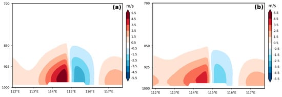
Figure 7.
Vertical profile of wind speed increment (m/s) on 30 June, 12 UTC 2022; before QC (a); after QC (b).
Figure 8 shows the analysis increase in wind speed at 850 hPa at the assimilation time. After assimilating the HY-2B data, the wind speeds on the west and south sides of the TC center had a significantly positive adjustment, whereas those on the east and north sides had negative adjustments. These adjustments changed the structure and path prediction of the typhoon. Simultaneously, the increment in the wind field was significantly reduced after processing, and the IRMCD QC method can weaken the influence introduced by the observation. Furthermore, this study found that the specific impact of assimilation was mainly reflected in the adjustment of divergence (Figure 9). After data processing, the increment in divergence at 850 hPa showed a clear negative convergence center near the the typhoon center. The divergence field was significantly weakened after QC but was still clear. Lower convergence levels can increase the strength of typhoons, which is beneficial for their development and maintenance.
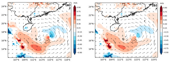
Figure 8.
Analysis of increment in wind speed (m/s) at the 850 hPa levels and 850 hPa horizontal wind vector on 30 June, 12 UTC 2022; before QC (a); after QC (b).
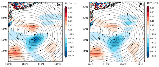
Figure 9.
Analysis of increment in divergence (s−1) in 850 hPa levels on 30 June, 12 UTC 2022; before QC (a); after QC (b).
4.3. Track and Intensity of Typhoon
Figure 10 shows the track and its accumulated errors. The simulation results of the track (Figure 10a) show that the deviation was largest 12 h before the typhoon lands, and the track before QC deviated the most in the three experiments, whereas it was steadier and the deviation was greatly reduced after QC. The track error (Figure 10b) increased with simulation time, and the improvement in the assimilation was not significant before QC, while the error was larger than that of the CTRL experiment in the last 12 h forecast. However, the accumulated error after processing with QC was always the smallest. This shows that HY-2B data without QC processing had a poor impact on track improvement or even a negative influence; however, the negative impact of the data could be eliminated by processing using the IRMCD method, and the track could be slightly improved.
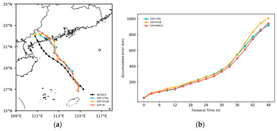
Figure 10.
Simulation of the track (a) and the accumulated error (b) of track from 30 June, 12 UTC to 2 July, 12 UTC 2022. The best track from IBTrACS (black line) and experiments for EXP-CTRL (green line), EXP-HY2B (yellow line), EXP-IRMCD (red line).
In terms of intensity, the variation in minimum sea level pressure (MSLP) with time indicates (Figure 11a) that the typhoon is a nearshore strengthening typhoon and reached its maximum intensity before landfall. In the intensity simulation, compared with the maximum wind speed (Figure 11b), the simulation result for the minimum pressure, which is also a commonly used physical quantity to characterize the intensity, was more significant. In contrast with the improvement in track location, the intensity before QC significantly improved, especially in the typhoon nearshore enhancement stage, which is often the most important period in the operational forecast. An adjustment after QC can further improve the intensity, and the value of the MSLP is closer to that observed.
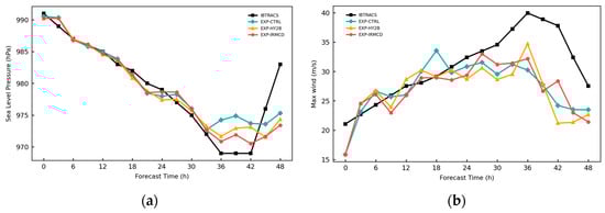
Figure 11.
Simulation of intensity, variation in minimum sea level pressure (MSLP, (a)), and maximum wind speed (b) from 30 June, 12 UTC to 2 July, 12 UTC 2022. The best track from IBTrACS (black line), the experiments for EXP-CTRL (green line), EXP-HY2B (yellow line), and EXP-IRMCD (red line).
To further explore the specific adjustment of QC during typhoon nearshore strengthening, this study obtained the period of enhancement by a 6 h pressure change. In Figure 12a, the pressure change below the magenta dotted line is equal to or less than −4.14 hPa; that is, the TC is determined to be a slow enhancement [35]. The figure shows that the simulation time between 27 and 36 h was the period of typhoon nearshore enhancement, and the vertical wind shear (VWS) changed significantly during this period (Figure 12b). In this study, the commonly used method, the wind speed difference between 200 and 850 hPa, was used to calculate VWS, and this value was represented by the average in a square area of 200 km around the typhoon center. The results showed that the VWS after QC significantly decreased after 27 h. After the two reduction processes, it reached a minimum during landfall and increased with strength recovery after landfall. A weak VWS is conducive to the maintenance of typhoon intensity [36,37]. Therefore, it was indicated that the QC algorithm can provide favorable atmospheric conditions for typhoon intensification by reducing the vertical wind shear.
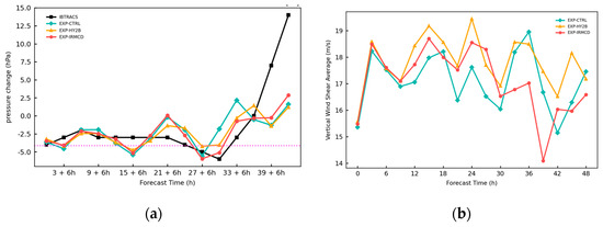
Figure 12.
The 6 h pressure change (a) and the vertical wind shear (VWS, (b)) in a square area of 200 km from 30 June, 12 UTC to 2 July, 12 UTC 2022. The pressure below the magenta dotted line is equal to or less than −4.14 hPa; the best track from IBTrACS (black line), the experiments for EXP-CTRL (green line), EXP-HY2B (yellow line), and EXP-IRMCD (red line).
5. Analysis
5.1. Profile of Moisture Flux Divergence and Vertical Velocity
The assimilation improvements in this study were mainly concentrated near the center of typhoon. The convergence of the average moisture flux divergence within 200 km of the typhoon center mainly occurred below 850 hPa (Figure 13), and there was a slight enhancement in low-level moisture flux convergence after QC. When the typhoon reached its strongest stage, there was an evident divergence center in the upper air. Compared to EXP-CTRL, the introduction of HY-2B data significantly increased the divergence and height (Figure 13c). Further enhancement in the quality-controlled (QCed) divergence in the upper air can strengthen the moisture flux convergence at lower levels, favoring the maintenance of the ascending motion (Figure 13e,f). The vertical velocity profile revealed a variation in speed at the location of minimum divergence (strongest convergence) near the center at 850 hPa during the peak typhoon intensity. In EXP-CTRL, the values of the vertical velocity below 700 hPa were negative, inhibiting the upward transport of water vapor. DA significantly enhanced the low-level velocities, whereas the QCed vertical velocity exhibited a pronounced increase at the upper levels, indicating that QC effectively improved intensity.
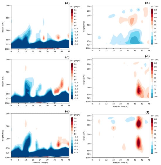
Figure 13.
Time series of moisture flux divergence (the first column, g/(kg*s)) and vertical velocity (the second column, m/s). The experiments for EXP-CTRL (a,b), EXP-HY2B (c,d), and EXP-IRMCD (e,f) on 1 July.
5.2. Horizontal Distribution of Vertical Wind Shear
Figure 14 shows the horizontal distribution of the VWS during typhoon enhancement. This indicates that the VWS was mainly primarily located around the center of typhoons. In EXP-CTRL, the high-value areas of the VWS at the three moments form a closed circle around the eye. The HY-2B data could change the distribution structure of VWS and break the closed ring structure, but the VWS strengthened and readjusted in local areas, and was distributed on both sides of the typhoon (Figure 14e,f). After QC, the high-value area of VWS and the intensity of surrounding wind shear were significantly weakened. Before the typhoon reached its greatest strength, the VWS was the weakest, and the range of the high-value area was the smallest (Figure 14i), indicating that the HY-2B data can adjust the wind field, improve the distribution of VWS, and prevent the convective suppression of typhoons in all directions. However, the strengthening and uneven distribution of the local VWS can easily lead to instability in the typhoon’s circulation structure and influence typhoon intensity. The IRMCD algorithm can significantly weaken the intensity of wind shear in high-value areas, while also weakening the wind shear intensity of the overall environmental wind field, which is conducive to maintaining the intensity.
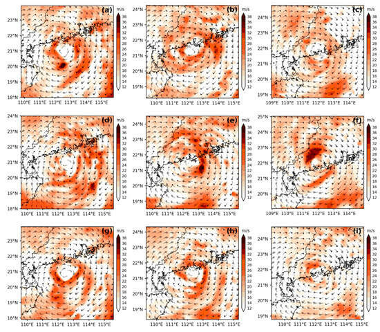
Figure 14.
Horizontal wind vector (500 hPa) and horizontal distribution of VWS (m/s) between 200 and 850 hPa. The experiments for EXP-CTRL (a–c), EXP-HY2B (d–f), and EXP-IRMCD (g–i) on 1 July, 21 UTC (the first column), 2 July, 00 UTC (the second column), and 03 UTC (the third column).
5.3. Vertical Profile of Typhoon
The profile shows the three moments when the typhoon reached its maximum strength (Figure 15 and Figure 16). The EXP-CTRL results showed that the momentum of the typhoon was mainly concentrated in the middle and lower layers, and that the flow field on both sides of the eye was unevenly distributed. The wind speeds on the east and north sides of the eye were high, and convection development in the upper layer was relatively weak. Therefore, the overall structure was unstable and not conducive to typhoon maintenance. The assimilation of HY-2B data could extend the impact of the forecast upward with the momentum obviously transmitted to the upper layer on the east and south sides of the typhoon at 00 UTC (Figure 15d and Figure 16d), and it was mainly on the east and north sides at the latter two moments, which was conducive to the convective development and energy exchange of the typhoon. However, at the latter two moments, before QC, the wind fields on the west and south sides of the typhoon center were unevenly distributed at different heights in the middle layer (Figure 15e and Figure 16f), causing an unstable barotropic structure, and the vertical structure of the eyewall was damaged. The forecast results after QC strengthened the upward momentum transport on the southern side of the typhoon (Figure 15g and Figure 16h,i). Meanwhile, the vertical structure of the eyewall was more obvious, and the barotropic structure was more stable (Figure 15h and Figure 16h,i). At the last moment (when the typhoon was strongest), the distribution of wind speed on the eyewall in the north and south was the most even at different heights (Figure 16i), which is conducive to a stable typhoon structure.
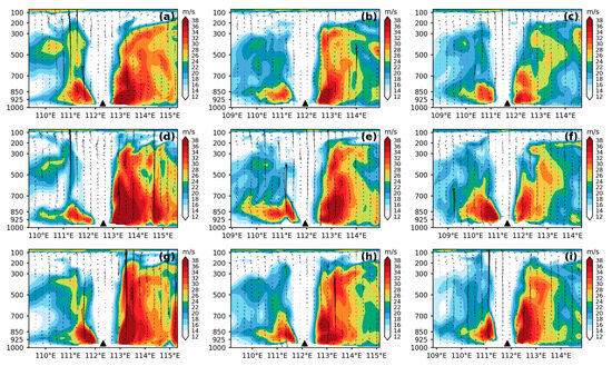
Figure 15.
Latitudinal vertical profile along the typhoon center. The experiments for EXP-CTRL (a–c), EXP-HY2B (d–f), and EXP-IRMCD (g–i) on 2 July, 00 UTC (the first column), 03 UTC (the second column), and 06 UTC (the third column). Shaded colors are horizontal wind speed (m/s) at different levels. The black triangle is the center of the typhoon at the surface.
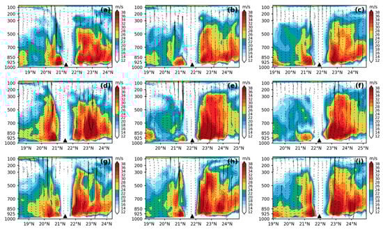
Figure 16.
Meridional vertical profile along the typhoon center. The experiments for EXP-CTRL (a–c), EXP-HY2B (d–f), and EXP-IRMCD (g–i) on 2 July, 00 UTC (the first column), 03 UTC (the second column), and 06 UTC (the third column). Shaded colors are the horizontal wind speed (m/s) at different levels. The black triangle is the center of the typhoon at the surface.
Overall, the HY-2B data strengthened the upward transport of momentum in the middle and lower layers of the typhoon, improving the distribution of VWS and enhancing convection. However, the data also induced an unstable flow field in the typhoon, which can explain why the forecast track improved slightly without QC, but the intensity improved. The unstable flow field can be improved by QC, and the algorithm can significantly weaken the wind shear, enhance convective transport, and improve intensity prediction.
6. Conclusions and Discussion
6.1. Conclusions
The HY-2B satellite is the first satellite of a marine dynamic environment monitoring system that can provide high-precision data for ocean observation and early warning. In previous experiments, QC application in assimilation ensured the stable prediction of numerical models; however, the IRMCD method, which is suitable for multivariate analysis, is mostly used in radar profile research, and the impact of QC on satellite wind vector data is not yet clear. In this study, to explore the QC effect of the IRMCD method in the HY-2B OWS assimilation application and improve the utilization efficiency of satellite data, the method was applied to the WRF model and GSI system to compare the forecasting results before and after QC.
IRMCD can significantly improve the Gaussian distribution of the OMB, with larger outliers eliminated by QC at both ends of the data, making it closer to a Gaussian distribution. The improvement in kurtosis was the most significant for the kurtosis and skewness indices, converging from 9.491/18.341 to −0.106/−0.156.
The analysis increment at the assimilation time shows that the wind field of HY-2B is the main adjustment variable, which is mainly concentrated at 850 hPa levels, with positive adjustments on the west and south sides of the typhoon center and negative adjustments on the east and north sides. Furthermore, this study also found that the observation could introduce a negative adjustment of the divergence near the typhoon center, which can be mitigated by the IRMCD method. In the forecasting results, the HY-2B data increased the track deviation, but the QC of the IRMCD method could eliminate the negative impact and improve it to a certain extent, and the observation of HY-2B could reduce the typhoon’s MSLP when its intensity reached its maximum, improving the prediction of intensity, as the IRMCD method could further improve the forecast effect on this basis.
From the perspective of energy, the QC algorithm can significantly strengthen the divergence of moisture flux in the upper layer, and with convergence in the lower layer, it is conducive to the upper transport of water vapor. Simultaneously, the vertical velocity near the typhoon center increased significantly at both high and low altitudes after QC, which was beneficial for the maintenance of typhoon intensity. Further research found that the IRMCD algorithm significantly reduced the VWS, particularly during the typhoon intensification stage. This reduction had a noticeable positive effect on typhoon intensity. In addition, HY-2B data can strengthen the upward transport of momentum in the middle and lower layers of the typhoon but also induce an unstable flow field, which can be improved by the IRMCD method. QC not only reduces VWS but is also beneficial to the stability of typhoon’s barotropic structures, further improving forecasting.
6.2. Discussion
The introduction of HY-2B data had both positive and negative contributions to the forecast, whereas the IRMCD improved the forecast results by eliminating the negative effects. However, to be widely used, the IRMCD method requires further investigation using different data and batch experiments. In addition, although the IRMCD method determines the observations around the typhoon center as outliers, which are often considered key data with precision information in forecasting operations, this does not mean that HY-2B data are unavailable in this region, and these may cause unstable forecasting for the model. Therefore, this method needs to be further explored to ensure effective QC while retaining important information. Finally, only the wind vectors of the HY-2B scatterometer were assimilated in this study, and observational data from different sources were assimilated in the actual forecasting operation. The correlation between different data and variables needs to be considered, which will result in more errors; therefore, it is worth discussing how the QC and forecast results will change.
Author Contributions
Conceptualization, Y.Z.; methodology, Y.Z. and J.H.; software, J.H., Y.Z., J.L. and D.S.; validation, D.S., Q.T. and J.F.; writing—original draft preparation, J.H.; writing—review and editing, Y.Z. and J.H.; supervision, Y.Z. and J.X.; project administration, Y.Z.; funding acquisition, Y.Z. All authors have read and agreed to the published version of the manuscript.
Funding
This study was jointly supported by the National Natural Science Foundation of China (42375159), National Natural Science Foundation of China (42130605), National Key R&D Program of China (2019YFC1510002) and program for scientific research start-up funds of Guangdong Ocean University (R20021).
Institutional Review Board Statement
Not applicable.
Informed Consent Statement
Not applicable.
Data Availability Statement
Data of HY-2B satellites were obtained from the website: “https://osdds.nsoas.org.cn (accessed on 19 April 2023)”. The authors of this paper would like to acknowledge the support provided by the National Satellite Ocean Application Service.
Acknowledgments
I would like to express my sincere gratitude to the following individuals for their valuable contributions to this research project. Zhang provided invaluable guidance and mentorship throughout the entire process, from the initial conceptualization to the final revision. I am also grateful to my research participants in the ‘GDOU-NWP’ group for their willingness to share their insights and experiences. Finally, I would like to thank my family and friends for their unwavering support and encouragement throughout this journey.
Conflicts of Interest
The authors declare no conflicts of interest.
References
- Guo, Q.Y.; Xu, X.Z.; Zhang, K.Y.; Li, Z.Q.; Huang, W.J.; Mansaray, L.R.; Liu, W.W.; Wang, X.Z.; Gao, J.; Huang, J.F. Assessing Global Ocean Wind Energy Resources Using Multiple Satellite Data. Remote Sens. 2018, 10, 100. [Google Scholar] [CrossRef]
- Christiansen, M.B.; Koch, W.; Horstmann, J.; Hasager, C.B.; Nielsen, M. Wind resource assessment from C-band SAR. Remote Sens. Environ. 2006, 105, 68–81. [Google Scholar] [CrossRef]
- Hasager, C.B.; Badger, M.; Peña, A.; Larsén, X.G.; Bingöl, F. SAR-Based Wind Resource Statistics in the Baltic Sea. Remote Sens. 2011, 3, 117–144. [Google Scholar] [CrossRef]
- Chang, R.; Zhu, R.; Badger, M.; Hasager, C.B.; Zhou, R.W.; Ye, D.; Zhang, X.W. Applicability of Synthetic Aperture Radar Wind Retrievals on Offshore Wind Resources Assessment in Hangzhou Bay, China. Energies 2014, 7, 3339–3354. [Google Scholar] [CrossRef]
- Meroni, A.N.; Desbiolles, F.; Pasquero, C. Satellite signature of the instantaneous wind response to mesoscale oceanic thermal structures. Q. J. R. Meteorol. Soc. 2023, 149, 3373–3382. [Google Scholar] [CrossRef]
- Stiles, B.W.; Yueh, S.H. Impact of rain on spaceborne Ku-band wind scatterometer data. IEEE Trans. Geosci. Remote Sens. 2002, 40, 1973–1983. [Google Scholar] [CrossRef]
- Chen, K.; Xie, X.; Zang, J.; Zou, J.; Zhang, Y. Accuracy analysis of the retrieved wind from HY-2B scatterometer. J. Trop. Oceanogr. 2020, 39, 30–40. [Google Scholar] [CrossRef]
- Lang, S.; Lin, W.; Zhang, Y.; Jia, Y. On the Quality Control of HY-2 Scatterometer High Winds. Remote Sens. 2022, 14, 5565. [Google Scholar] [CrossRef]
- Zhao, K.; Zhao, C.; Chen, G. Evaluation of Chinese Scatterometer Ocean Surface Wind Data: Preliminary Analysis. Earth Space Sci. 2021, 8, e2020EA001482. [Google Scholar] [CrossRef]
- Wang, Z.; Stoffelen, A.; Zou, J.; Lin, W.; Verhoef, A.; Zhang, Y.; He, Y.; Lin, M. Validation of New Sea Surface Wind Products from Scatterometers Onboard the HY-2B and MetOp-C Satellites. IEEE Trans. Geosci. Remote Sens. 2020, 58, 4387–4394. [Google Scholar] [CrossRef]
- Li, X.; Yang, J.; Wang, J.; Han, G. Evaluation and Calibration of Remotely Sensed High Winds from the HY-2B/C/D Scatterometer in Tropical Cyclones. Remote Sens. 2022, 14, 4654. [Google Scholar] [CrossRef]
- Wang, J.; Jiang, X.; Shen, X.; Zhang, Y.; Wan, X.; Han, W.; Wang, D. Assimilation of Ocean Surface Wind Data by the HY-2B Satellite in GRAPES: Impacts on Analyses and Forecasts. Adv. Atmos. Sci. 2022, 40, 44–61. [Google Scholar] [CrossRef]
- Liu, S.; Lin, W.; Portabella, M.; Wang, Z. Characterization of Tropical Cyclone Intensity Using the HY-2B Scatterometer Wind Data. Remote Sens. 2022, 14, 1035. [Google Scholar] [CrossRef]
- Liu, S.; Lin, W.; Wang, Z.; Lang, S. Determination of tropical cyclone location and intensity using HY-2B scatterometer data. Haiyang Xuebao 2021, 43, 146–156. [Google Scholar] [CrossRef]
- Xu, Z.; Wang, Y.; Fan, G. A Two-Stage Quality Control Method for 2-m Temperature Observations Using Biweight Means and a Progressive EOF Analysis. Mon. Weather Rev. 2013, 141, 798–808. [Google Scholar] [CrossRef]
- Kubecka, P. A possible world record maximum natural ground surface temperature. Weather 2001, 56, 218–221. [Google Scholar] [CrossRef]
- D MEEK, J.H. Data quality checking for single station meteorological databases. Agric. For. Meteorol 1994, 69, 85–109. [Google Scholar] [CrossRef]
- Allen, R.G.; Pereira, L.S.; Raes, D.; Smith, M. Crop evapotranspiration-Guidelines for computing crop water requirements-FAO Irrigation and drainage paper 56. Food Agric. Organ. United Nations 1998, 300, D05109. [Google Scholar]
- Gleason, B. National Climatic Data Center data documentation for data set 9101. Glob. Dly. Climatol. Netw. Version 1 2002, 1, 26. [Google Scholar]
- Feng, S.; Hu, Q.; Qian, W.H. Quality control of daily meteorological data in China, 1951–2000: A new dataset. Int. J. Climatol. 2004, 24, 853–870. [Google Scholar] [CrossRef]
- Lin, W.; Portabella, M.; Stoffelen, A.; Verhoef, A.; Turiel, A. ASCAT Wind Quality Control Near Rain. IEEE Trans. Geosci. Remote Sens. 2015, 53, 4165–4177. [Google Scholar] [CrossRef]
- Lin, W.; Portabella, M.; Turiel, A.; Stoffelen, A.; Verhoef, A. An Improved Singularity Analysis for ASCAT Wind Quality Control: Application to Low Winds. IEEE Trans. Geosci. Remote Sens. 2016, 54, 3890–3898. [Google Scholar] [CrossRef]
- Lanzante, J.R. Resistant, robust and non-parametric techniques for the analysis of climate data: Theory and examples, including applications to historical radiosonde station data. Int. J. Climatol. A J. R. Meteorol. Soc. 1996, 16, 1197–1226. [Google Scholar] [CrossRef]
- Li, J.; Zou, X. A Quality Control Procedure for FY-3A MWTS Measurements with Emphasis on Cloud Detection Using VIRR Cloud Fraction. J. Atmos. Ocean. Technol. 2013, 30, 1704–1715. [Google Scholar] [CrossRef][Green Version]
- Xu, C.; Wang, J.; Hu, M.; Li, Q. Estimation of Uncertainty in Temperature Observations Made at Meteorological Stations Using a Probabilistic Spatiotemporal Approach. J. Appl. Meteorol. Climatol. 2014, 53, 1538–1546. [Google Scholar] [CrossRef][Green Version]
- Wang, X.; Lin, Y.; Liu, D.; Lin, L. Comparative analysis of two data quality control methods for wind profile radar to numerical assimilation. J. Meteorol. Sci. 2022, 42, 495–505. [Google Scholar]
- Zhang, Y.; Chen, M.; Zhong, J. A Quality Control Method for Wind Profiler Observations toward Assimilation Applications. J. Atmos. Ocean. Technol. 2017, 34, 1591–1606. [Google Scholar] [CrossRef]
- Rousseeuw, P.J. Least Median of Squares Regression. J. Am. Stat. Assoc. 1984, 79, 871–880. [Google Scholar] [CrossRef]
- Rousseeuw, P.J. Multivariate estimation with high breakdown point. Math. Stat. Appl. 1985, 8, 283–297. [Google Scholar]
- Rousseeuw, P.J.; Driessen, K.V. A Fast Algorithm for the Minimum Covariance Determinant Estimator. Technometrics 1999, 41, 212–223. [Google Scholar] [CrossRef]
- Hawkins, D.M.; Olive, D.J. Improved feasible solution algorithms for high breakdown estimation. Comput. Stat. Data Anal. 1999, 30, 1–11. [Google Scholar] [CrossRef]
- Cerioli, A. Multivariate Outlier Detection With High-Breakdown Estimators. J. Am. Stat. Assoc. 2010, 105, 147–156. [Google Scholar] [CrossRef]
- de Kloe, J.; Stoffelen, A.; Verhoef, A. Improved Use of Scatterometer Measurements by Using Stress-Equivalent Reference Winds. IEEE J. Sel. Top. Appl. Earth Obs. Remote Sens. 2017, 10, 2340–2347. [Google Scholar] [CrossRef]
- KNMI Scatterometer Team. NSCAT-4 Geophysical Model Function. Available online: https://scatterometer.knmi.nl/nscat4_gmf/ (accessed on 19 April 2023).
- Yu, Y.; Yao, X. A Statistical Analysis on Intensity Change of Tropical Cyclone over the Western North Pacific. J. Trop. Meteorol. 2006, 22, 521–526. [Google Scholar] [CrossRef]
- Frank, W.M.; Ritchie, E.A. Effects of environmental flow upon tropical cyclone structure. Mon. Weather. Rev. 1999, 127, 2044–2061. [Google Scholar] [CrossRef]
- Frank, W.M.; Ritchie, E.A. Effects of vertical wind shear on the intensity and structure of numerically simulated hurricanes. Mon. Weather. Rev. 2001, 129, 2249–2269. [Google Scholar] [CrossRef]


Disclaimer/Publisher’s Note: The statements, opinions and data contained in all publications are solely those of the individual author(s) and contributor(s) and not of MDPI and/or the editor(s). MDPI and/or the editor(s) disclaim responsibility for any injury to people or property resulting from any ideas, methods, instructions or products referred to in the content. |
© 2024 by the authors. Licensee MDPI, Basel, Switzerland. This article is an open access article distributed under the terms and conditions of the Creative Commons Attribution (CC BY) license (https://creativecommons.org/licenses/by/4.0/).