
Fiber Lidar for Control of the Ecological State of the Atmosphere
Abstract
:1. Introduction
2. Fiber Lidar Framework
2.1. Block Diagram of Fiber Lidar
2.2. Lidar Sensing Equation
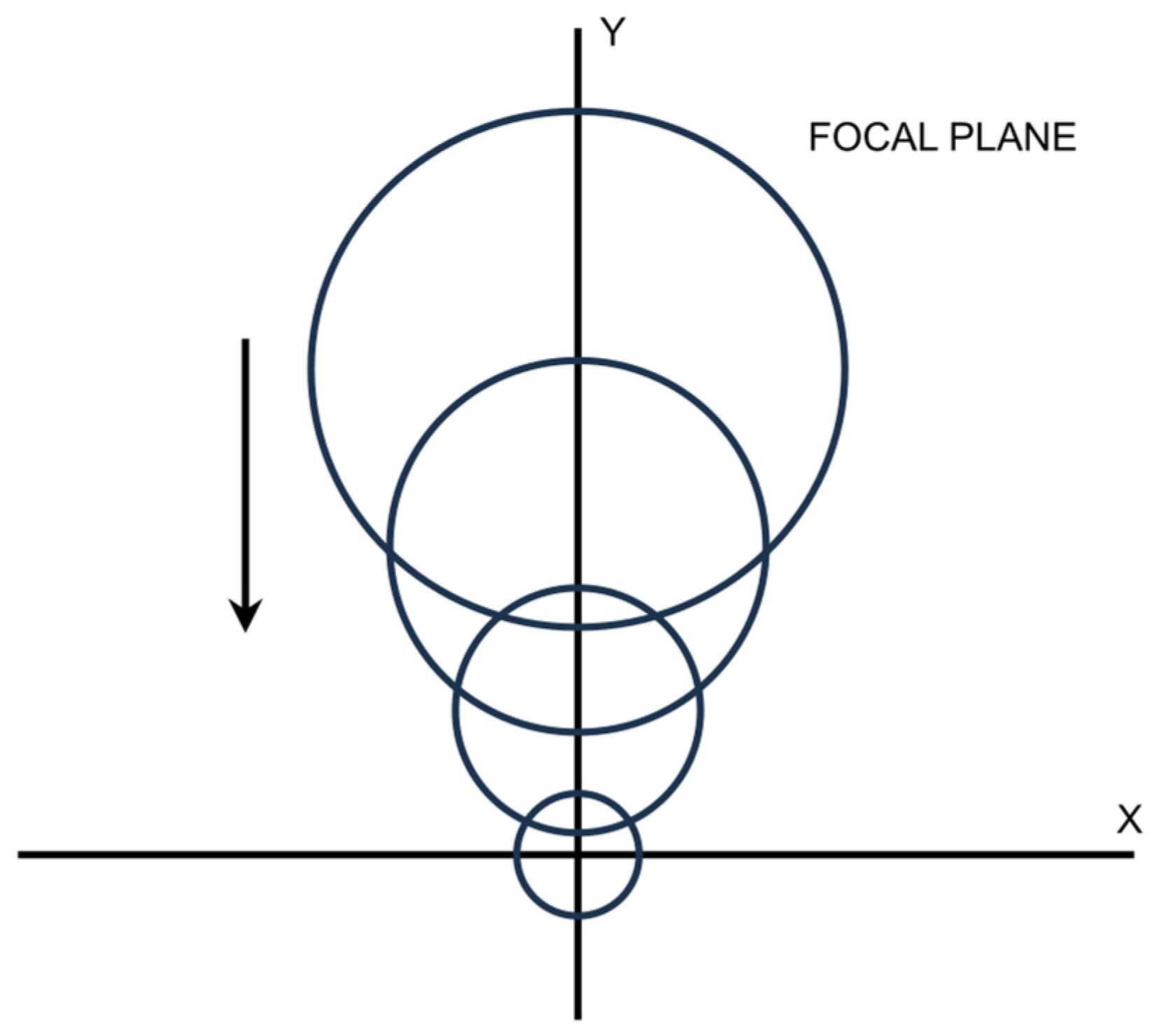
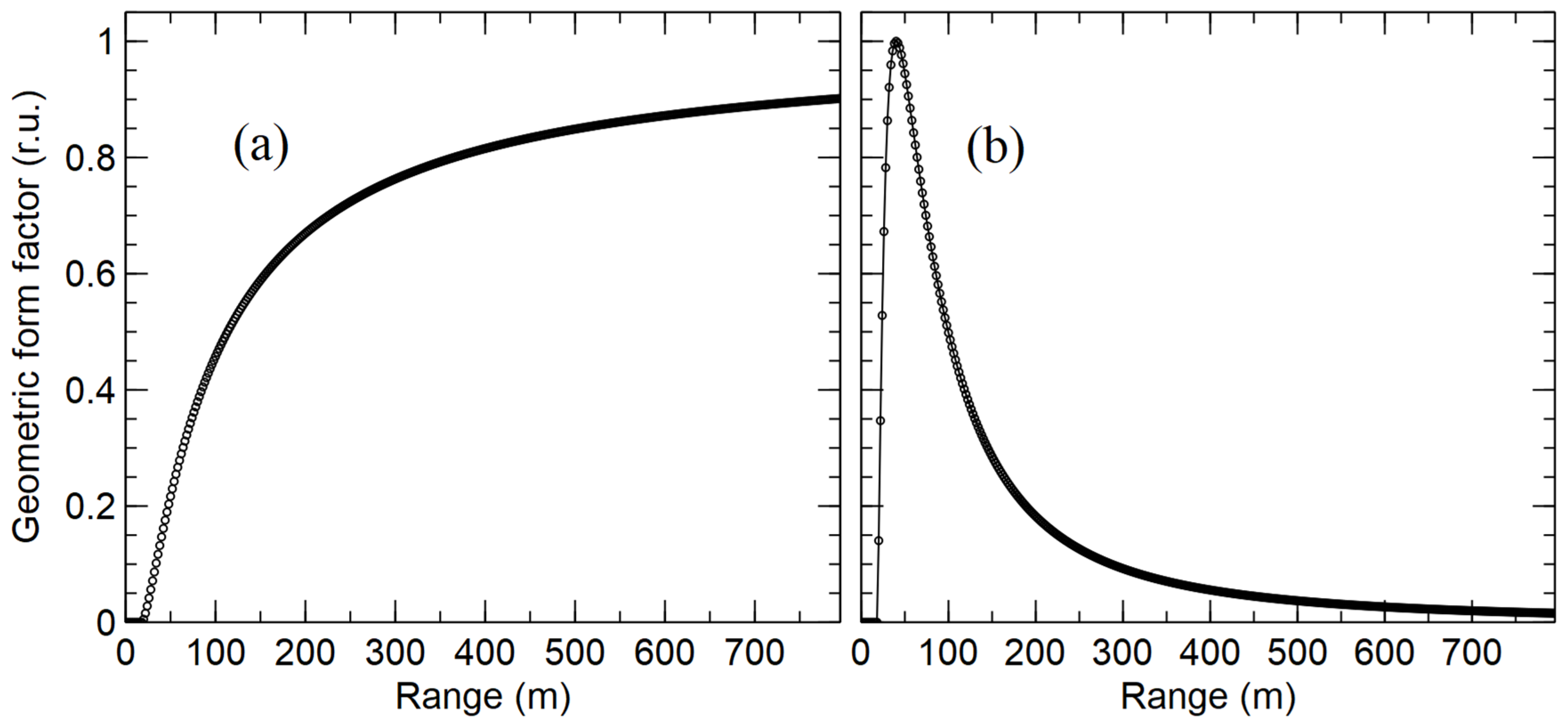
Geometric Form Factor of Fiber Lidar
3. Methods
3.1. Reference Signal Method
3.2. Lidar Signal Inversion Method
3.3. Data Processing of Measurement Results
4. Materials
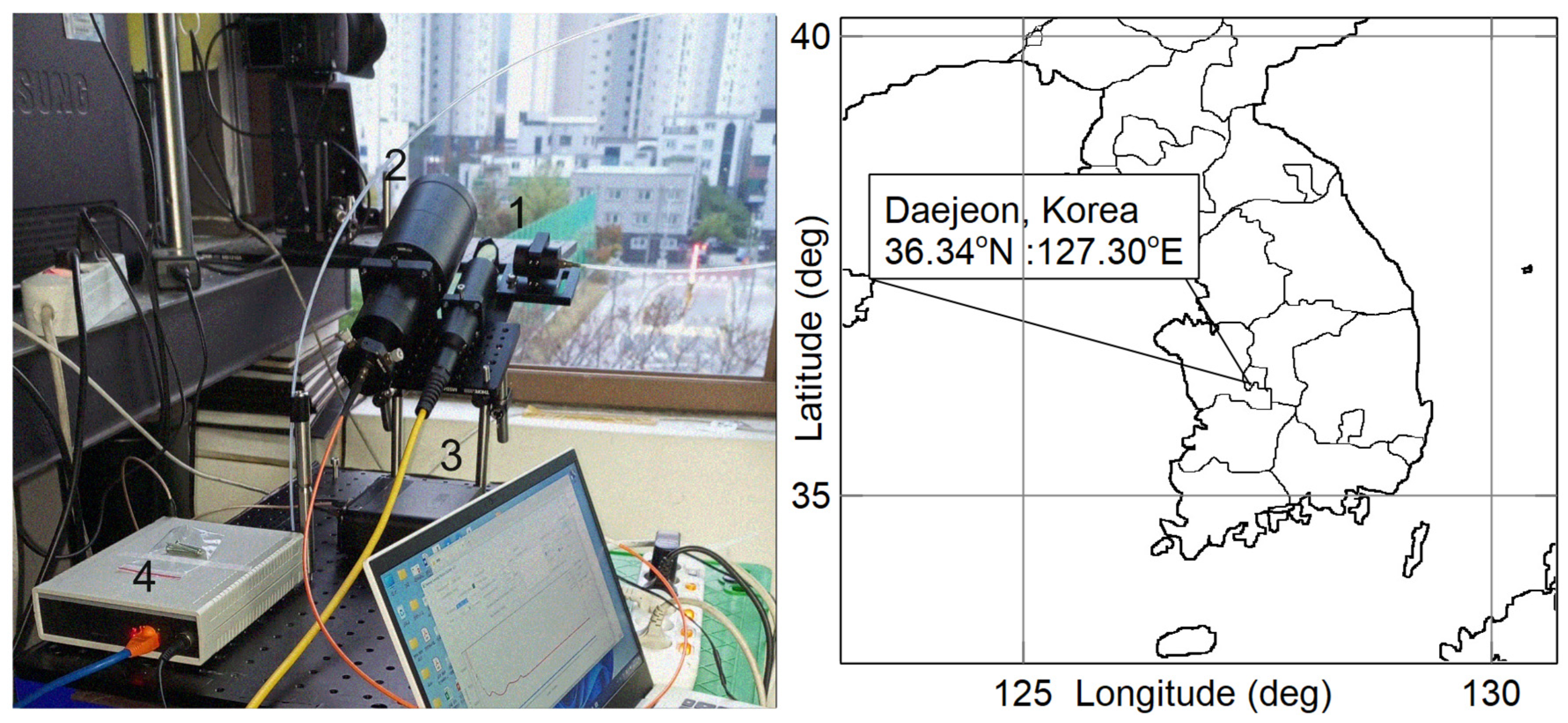
4.1. System
4.2. Sequence of Operations
5. Results
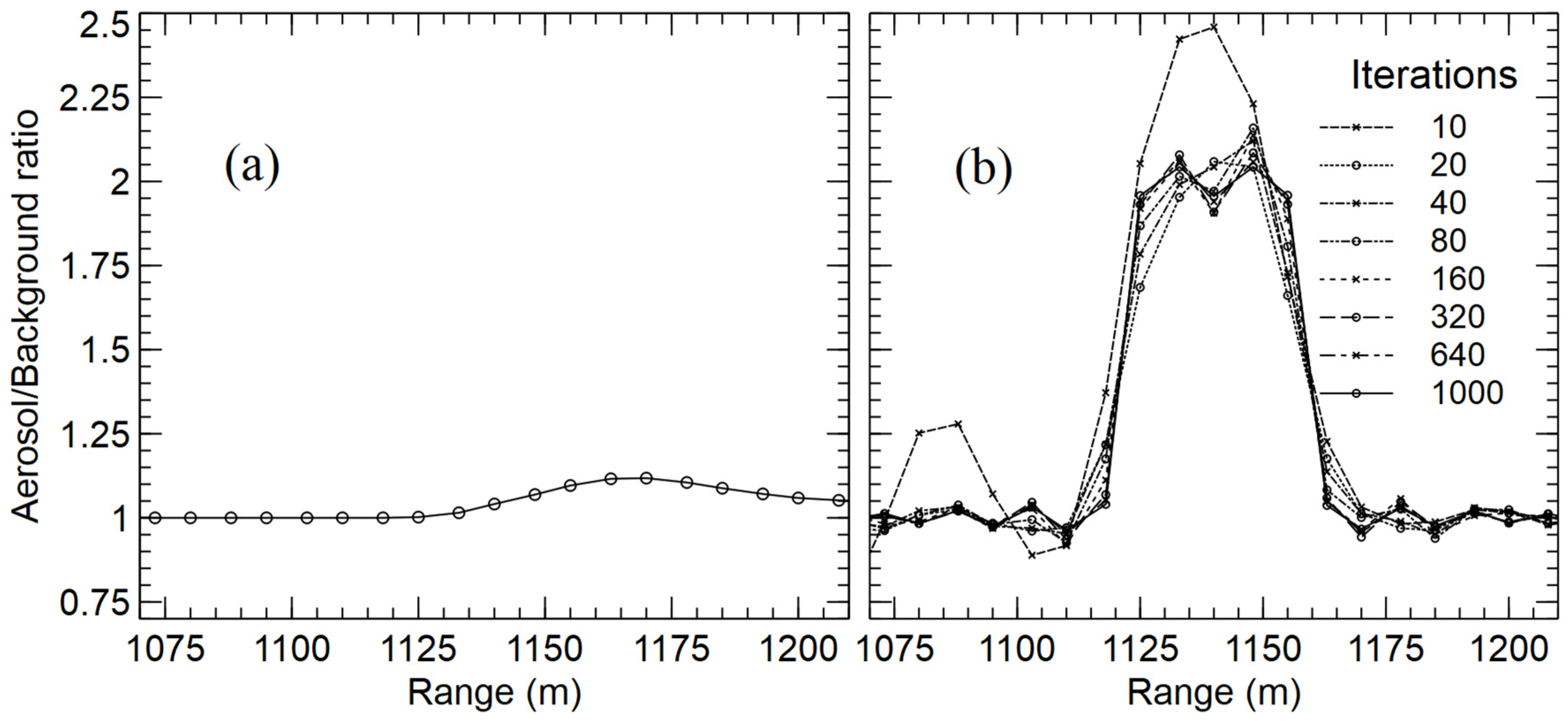
5.1. Verification
- Lidar return signals from the short-transmitted laser pulse with a duration equal to the resolution of the registration lidar system were formed.
- A square wave signal lasting several strobes was added to one of the signals. It simulated the occurrence of an aerosol impurity within the sensing range. As a result, two lidar signals were formed. A lidar signal without the impurity was designated as the reference signal . The lidar signal with the impurity was designated as .
- Lidar responses from the long laser pulse were formed. Calculations were carried out with Equation (16) as the convolution operation. The signals and , and the laser impulse transfer function took part in the calculations. As a result, lidar signals and were obtained.
5.2. Outdoor Experiment
- Control of the temporal stability of the fiber laser;
- Alignment of the fiber lidar and carrying out test measurements in the atmosphere;
- Carrying out the outdoor experiment;
- Experimental data processing;
- Reconstruction of lidar signals using the LSIM;
- Obtaining the measurement results with the RSM.
5.2.1. Control of the Temporal Stability of the Fiber Laser
5.2.2. Alignment of the Fiber Lidar and Carrying Out Test Measurements in the Atmosphere
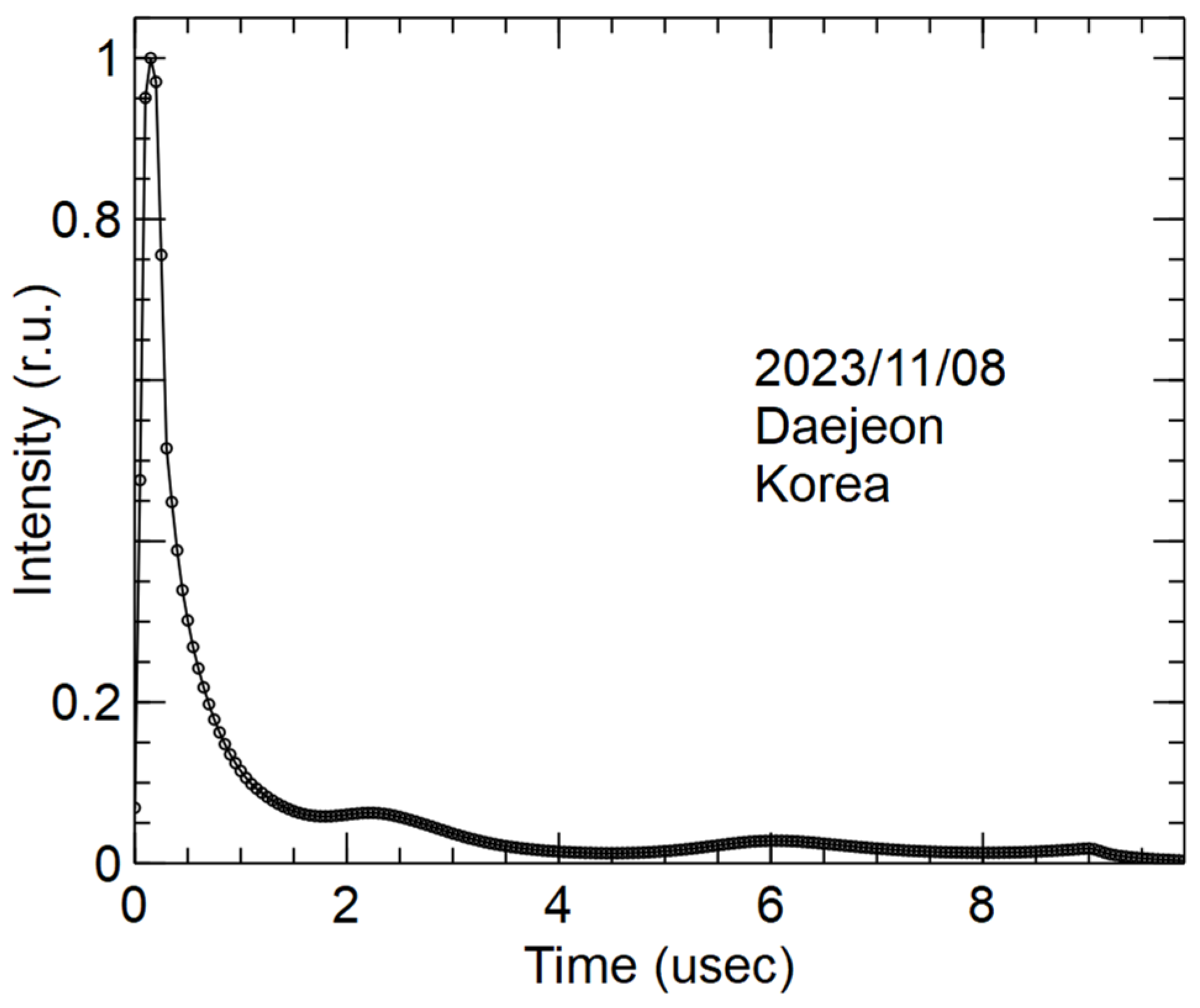
5.2.3. Carrying Out the Outdoor Experiment
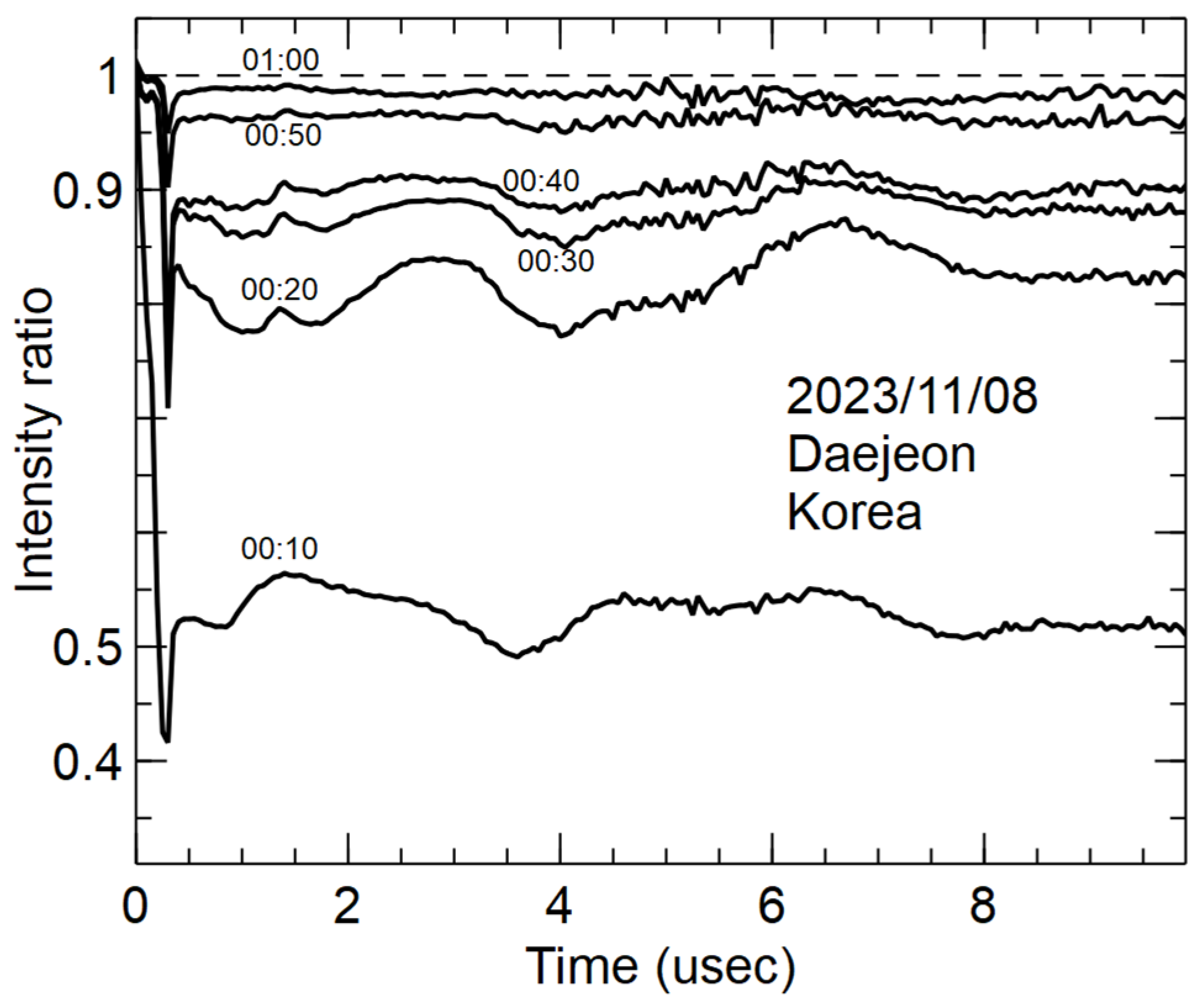
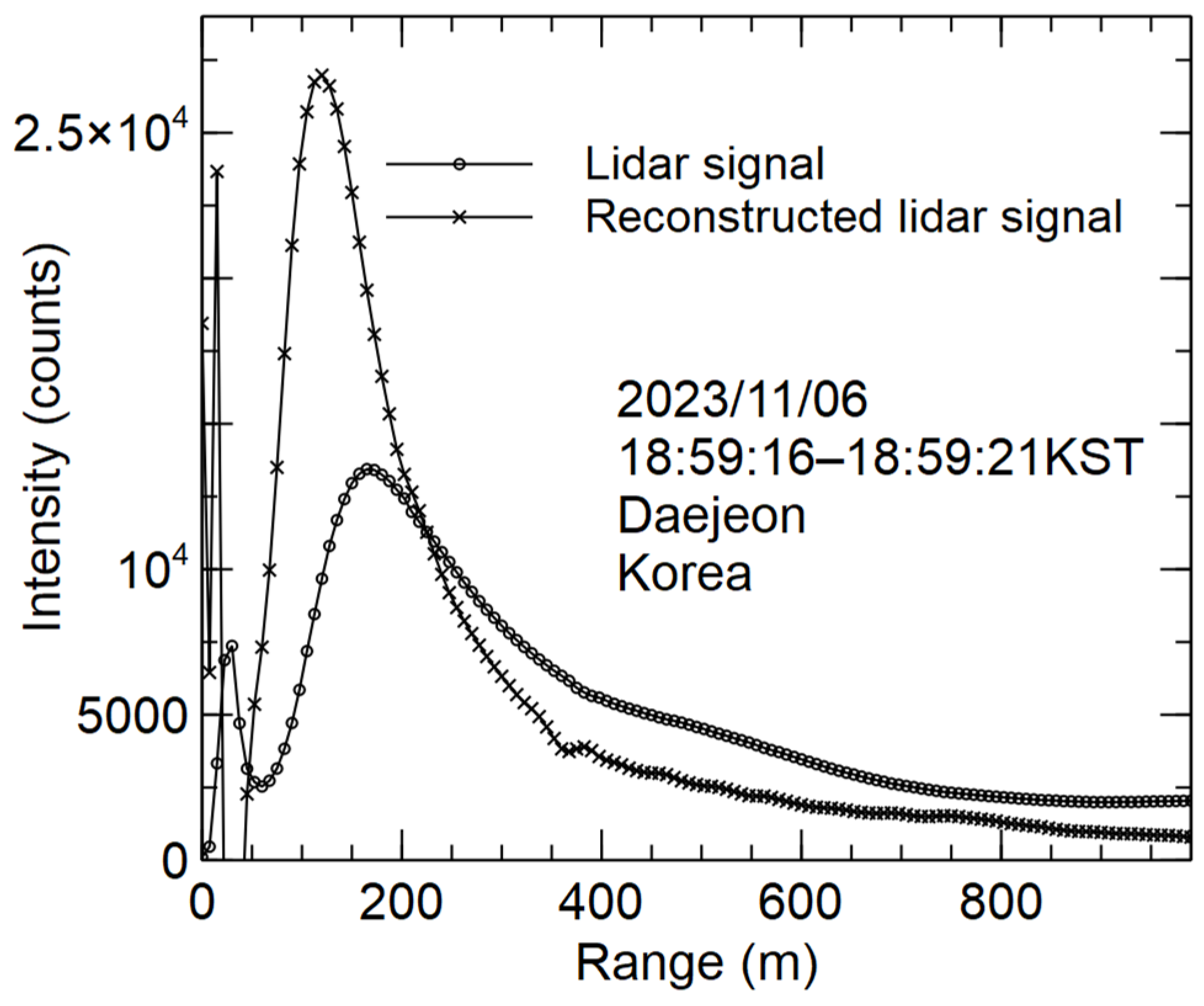
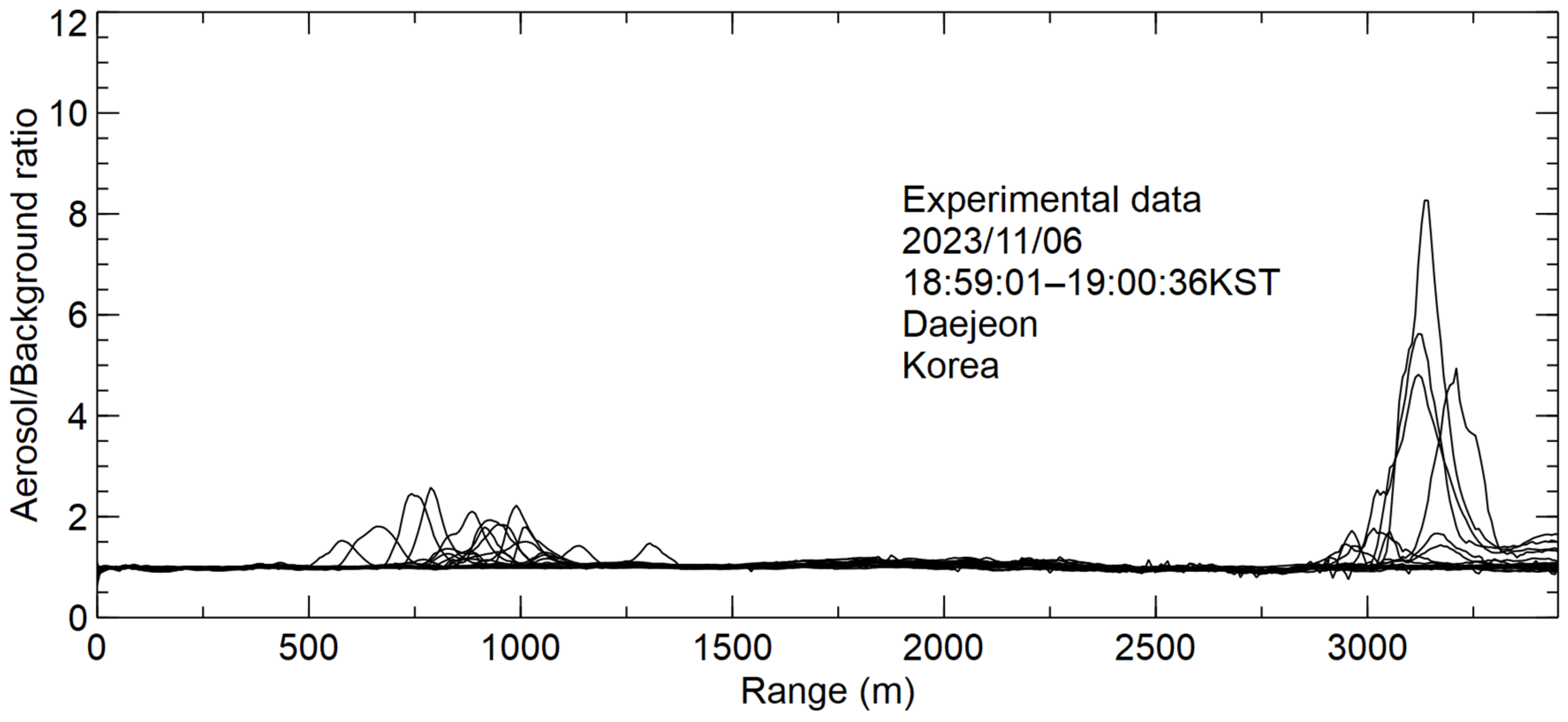
5.2.4. Experimental Data Processing
5.2.5. Reconstruction of the Lidar Signals Using the LSIM
6. Discussion
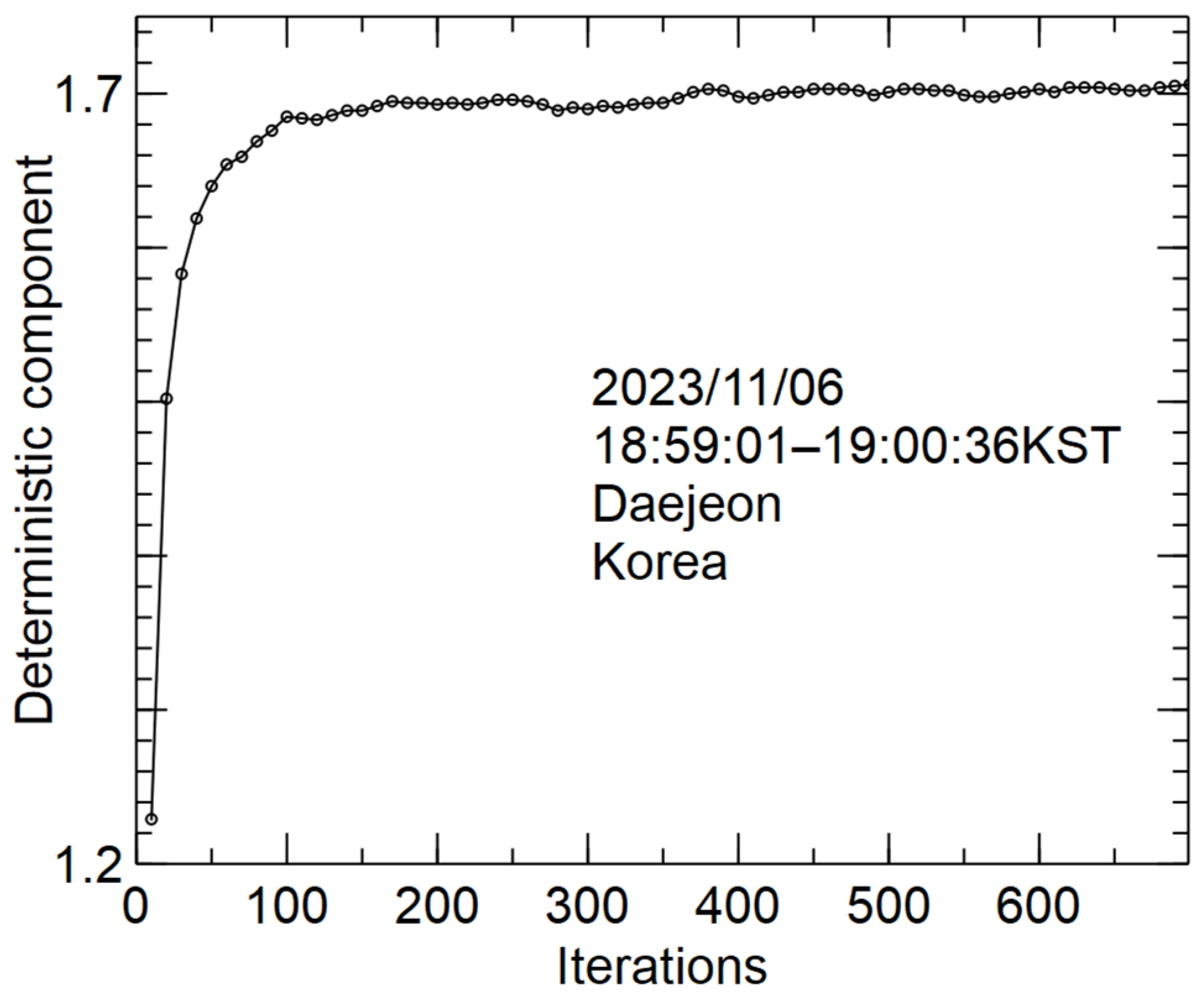
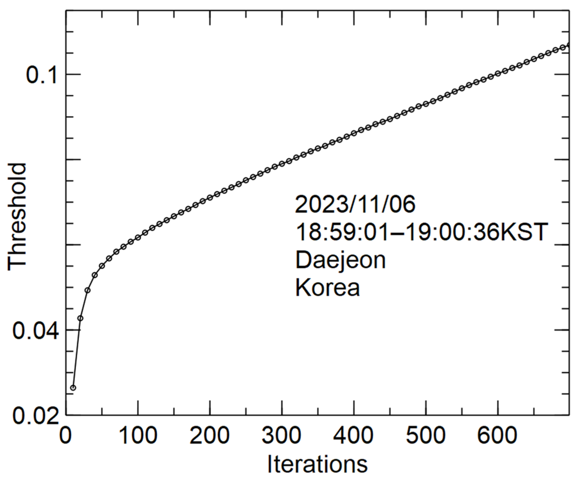
Criterion Selection in the LSIM
7. Conclusions
Author Contributions
Funding
Institutional Review Board Statement
Informed Consent Statement
Data Availability Statement
Conflicts of Interest
References
- Liu, Z.; Sugimoto, N.; Murayama, T. Extinction-to-backscatter ratio of Asian dust observed with high-spectral-resolution lidar and Raman lidar. Appl. Opt. 2002, 41, 2760–2767. [Google Scholar] [CrossRef] [PubMed]
- Ansmann, A.; Bösenberg, J.; Chaikovsky, A.; Comeron, A.; Eckhardt, S.; Eixmann, R.; Freudenthaler, V.; Ginoux, P.; Komguem, L.; Linné, H.; et al. Long-range transport of Saharan dust to northern Europe: The 11–16 October 2001 outbreak observed with EARLINET. J. Geophys. Res. 2003, 108, 4783. [Google Scholar] [CrossRef]
- Sakai, T.; Nagai, T.; Nakazato, M.; Mano, Y.; Matsumura, T. Ice clouds and Asian dust studied with lidar measurements of particle extinction-to-backscatter ratio, particle depolarization, and water-vapor mixing ratio over Tsukuba. Appl. Opt. 2003, 42, 7103–7116. [Google Scholar] [CrossRef]
- Shi, T.; Peng, Y.; Ma, X.; Han, G.; Zhang, H.; Pei, Z.; Li, S.; Mao, H.; Zhang, X.; Gong, W. China’s “coal-to-gas” policy had large impact on PM1.0 distribution during 2016–2019. J. Environ. Manag. 2024, 359, 121071. [Google Scholar] [CrossRef] [PubMed]
- Volkov, S.N.; Zaitsev, N.G.; Park, S.-H.; Kim, D.-H.; Noh, Y.-M. Lidar for the study of Asian dust in the near IR range of laser radiation. In Proceedings of the 30th International Conference Atmospheric and Ocean Optics, Atmospheric Physics, (AOO—2024), Saint Petersburg, Russia, 1–5 July 2024; Available online: https://symp.iao.ru/files/symp/aoo/30/ru/abstr_16104.pdf (accessed on 5 May 2024).
- Mishchenko, M.I.; Rosenbush, V.K.; Kiselev, N.N.; Lupishko, D.F.; Tishkovets, V.P.; Kaydash, V.G.; Belskaya, I.N.; Efimov, Y.S.; Shakhovskoy, N.M. Polarimetric Remote Sensing of Solar System Bodies; Akedemperoidyka: Kyiv, Ukraine, 2010; p. 291. [Google Scholar]
- Du, W.; Xin, J.; Wang, M.; Gao, Q.; Li, Z.; Wang, Y. Photometric measurements of spring aerosol optical properties in dust and non-dust periods in China. Atmos. Environ. 2008, 42, 7981–7987. [Google Scholar] [CrossRef]
- Noh, Y.-M.; Lee, K.-H.; Choi, Y.-J.; Kim, K.-R.; Lee, H.-L.; Choi, T.-J. Instantaneous Monitoring of Pollen Distribution in the Atmosphere by Surface-Based Lidar. Korean J. Remote Sens. 2012, 28, 1–9. [Google Scholar] [CrossRef]
- Shin, S.; Shin, D.; Lee, K.-H.; Noh, Y.-M. Classification of Dust/Non-dust Particle from the Asian Dust Plumes and Retrieval of Microphysical Properties using Raman Lidar System. J. Korean Soc. Atmos. Environ. 2012, 28, 688–696. [Google Scholar] [CrossRef]
- Sugimoto, N.; Huang, Z. Lidar methods for observing mineral dust. J. Meteorol. Res. 2014, 28, 173–184. [Google Scholar] [CrossRef]
- Volkov, S.N.; Samokhvalov, I.V.; Cheong, D.-H.; Kim, D.-H. Investigation of East Asian clouds with polarization light detection and ranging. Appl. Opt. 2015, 54, 3095–3105. [Google Scholar] [CrossRef]
- Eitel, J.; Höfle, B.; Vierling, L.A.; Abellán, A.; Asner, G.P.; Deems, J.S.; Glennie, C.L.; Joerg, P.C.; LeWinter, A.L.; Magney, T.S. Beyond 3-D: The new spectrum of LiDAR applications for earth and ecological sciences. Remote Sens. Environ. 2016, 186, 372–392. [Google Scholar] [CrossRef]
- Kawai, K.; Kai, K.; Jin, Y.; Sugimoto, N.; Batdorj, D. Lidar Network Observation of Dust Layer Development over the Gobi Desert in Association with a Cold Frontal System on 22–23 May 2013. J. Meteorol. Soc. Jpn. 2018, 96, 255–268. [Google Scholar] [CrossRef]
- Tsekeri, A.; Amiridis, V.; Louridas, A.; Georgoussis, G.; Freudenthaler, V.; Metallinos, S.; Doxastakis, G.; Gasteiger, J.; Siomos, N.; Paschou, P.; et al. Polarization lidar for detecting dust orientation: System design and calibration. Atmos. Meas. Tech. 2021, 14, 7453–7474. [Google Scholar] [CrossRef]
- Huang, Z.; Li, M.; Bi, J.; Shen, X.; Zhang, S.; Liu, Q. Small lidar ratio of dust aerosol observed by Raman-polarization lidar near desert sources. Opt. Express 2023, 31, 16909–16919. [Google Scholar] [CrossRef] [PubMed]
- Kuchinskaia, O.; Penzin, M.; Bordulev, I.; Kostyukhin, V.; Bryukhanov, I.; Ni, E.; Doroshkevich, A.; Zhivotenyuk, I.; Volkov, S.; Samokhvalov, I. Artificial Neural Networks for Determining the Empirical Relationship between Meteorological Parameters and High-Level Cloud Characteristics. Appl. Sci. 2024, 14, 1782. [Google Scholar] [CrossRef]
- Koroshetz, J.E. Fiber Lasers for Lidar. In Proceedings of the Optical Fiber Communication Conference and Exposition and the National Fiber Optic Engineers Conference, Anaheim, CA, USA, 6–11 March 2005; Technical Digest, CD, OFJ4. Optica Publishing Group: Washington, DC, USA, 2005. [Google Scholar]
- Cariou, J.-P.; Augere, B.; Valla, M. Laser source requirements for coherent lidars based on fiber technology. Comptes Rendus Phys. 2006, 7, 213–223. [Google Scholar] [CrossRef]
- Liu, J.; Zhu, X.; Diao, W.; Zhang, X.; Liu, Y.; Bi, D.; Jiang, L.; Shi, W.; Zhu, X.; Chen, W. All-Fiber Airborne Coherent Doppler Lidar to Measure Wind Profiles. EPJ Web Conf. 2016, 119, 10002. [Google Scholar] [CrossRef]
- Liu, H.; Zhu, X.; Fan, C.; Bi, D.; Liu, J.; Zhang, X.; Zhu, X.; Chen, W. Field Performance of All-Fiber Pulsed Coherent Doppler Lidar. EPJ Web Conf. 2020, 237, 08009. [Google Scholar] [CrossRef]
- Wulfmeyer, V.; Bosenberg, J. Single-mode operation of an injection-seeded alexandrite ring laser for application in water-vapor and temperature differential absorption lidar. Opt. Lett. 1996, 21, 1150–1152. [Google Scholar] [CrossRef]
- Zervas, M.N.; Codemard, C.A. High Power Fiber Lasers: A Review. IEEE J. Sel. Top. Quantum Electron. 2014, 20, 219–241. [Google Scholar] [CrossRef]
- Available online: https://www.xtlaser.com/mopa-technology-q-switching-technology/ (accessed on 29 April 2024).
- Halldórsson, T.; Langerholc, J. Geometrical form factors for the lidar function. Appl. Opt. 1978, 17, 240–244. [Google Scholar] [CrossRef]
- Harms, J. Lidar return signals for coaxial and noncoaxial systems with central obstruction. Appl. Opt. 1979, 18, 1559–1566. [Google Scholar] [CrossRef] [PubMed]
- Sasano, Y.; Shimizu, H.; Takeuchi, N.; Okuda, M. Geometrical form factor in the laser radar equation: An experimental determination. Appl. Opt. 1979, 18, 3908–3910. [Google Scholar] [CrossRef] [PubMed]
- Sassen, K.; Dodd, G.C. Lidar crossover function and misalignment effects. Appl. Opt. 1982, 21, 3162–3165. [Google Scholar] [CrossRef] [PubMed]
- Young, S.A. Lidar system optical alignment and its verification. Appl. Opt. 1987, 26, 1612–1616. [Google Scholar] [CrossRef]
- Noh, Y.-M.; Muller, D.; Shin, D.-H.; Lee, K.-H. Retrieval of Lidar Overlap Factor using Raman Lidar System. J. Korean Soc. Atmos. Environ. 2009, 25, 450–458. [Google Scholar] [CrossRef]
- Adam, M.; Marenco, F. Overlap correction function based on multi-angle measurements for an airborne direct-detection lidar for atmospheric sensing. Opt. Express 2024, 32, 11022–11040. [Google Scholar] [CrossRef] [PubMed]
- Available online: https://mathworld.wolfram.com/Circle-CircleIntersection.html (accessed on 17 April 2024).
- Kaczmarz, S. Angenäherte Auflösung von Systemen linearer Gleichungen. Bull. Pol. Acad. Sci. Tech. Sci. 1937, 19, 355–357. [Google Scholar]
- Kaczmarz, S. Approximate solution of systems of linear equations. Int. J. Control 1993, 57, 1269–1271. [Google Scholar] [CrossRef]
- Strohmer, T.; Vershynin, R. A Randomized Kaczmarz Algorithm with Exponential Convergence. J. Fourier Anal. Appl. 2009, 15, 262–278. [Google Scholar] [CrossRef]
- Censor, Y.; Eggermont, P.P.B.; Gordon, D. Strong underrelaxation in Kaczmarz’s method for inconsistent linear systems. Numer. Math. 1983, 41, 83–92. [Google Scholar] [CrossRef]
- Hanke, M.; Niethammer, W. On the acceleration of Kaczmarz’s method for inconsistent linear systems. Lin. Alg. Appl. 1990, 130, 83–98. [Google Scholar] [CrossRef]
- Gordon, R.; Bender, R.; Herman, G.T. Algebraic Reconstruction Techniques (ART) for three-dimensional electron microscopy and X-ray photography. J. Theor. Biol. 1970, 29, 477–481. [Google Scholar] [CrossRef] [PubMed]
- Herman, G.T.; Meyer, L.B. Algebraic reconstruction techniques can be made computationally efficient. IEEE Trans. Med. Imaging 1993, 12, 600–609. [Google Scholar] [CrossRef] [PubMed]
- Volkov, S.N.; Kaul, B.V.; Shelefontuk, D.I. Optimal method of linear regression in laser remote sensing. Appl. Opt. 2002, 41, 5078–5083. [Google Scholar] [CrossRef] [PubMed]
- Eadie, W.T.; Dryard, D.; James, F.E.; Roos, M.; Sadoulet, B. Statistical Methods in Experimental Physics; North-Holland Publishing Company: Amsterdam, The Netherlands, 1971; p. 296. [Google Scholar]
- Available online: https://en.maxphotonics.com/ (accessed on 7 April 2024).
- Hanke, M.; Niethammer, W. On the use of small relaxation parameters in Kaczmarz’s method. Z. Angew. Math. Mech. 1990, 70, 575–576. [Google Scholar]
- Needell, D. Randomized Kaczmarz solver for noisy linear systems. BIT Numer. Math. 2010, 50, 395–403. [Google Scholar] [CrossRef]


| Laser | Brand | MFP 20W, Maxphotonics (Shenzhen, China) |
| Type | Q-switch fiber laser | |
| Central wavelength (CWL) | 1064 nm | |
| Spectrum width, (FWHM) | 5 nm | |
| Pulse duration *, (FWHM) | 100 ns | |
| Pulse repetition rate | 30 kHz | |
| Pulse energy | 0.75 mJ | |
| Beam quality (M2) | 1.3 | |
| Beam divergence | <1 mrad | |
| Beam diameter | 7 mm | |
| Receiver | Type | Single plano-convex lens |
| Effective diameter | 60 mm | |
| Focal length | 300 mm | |
| Signal Processing | Model | EBAZ4205 controller |
| Type | Pulse counter | |
| Operation mode | Accumulation | |
| Strobe period | 50 ns | |
| Sensor N1 | Brand | SPCM AQRH13FC, Excelitas (Gaithersburg, MD, USA) |
| Type | Si-APD | |
| Operating mode | Single photon counting | |
| Active diameter | 100 µm | |
| Output fiber diameter | 100 µm | |
| Filter | Brand | FLH1064-3, Thorlabs (Newton, NJ, USA) |
| Type | Bandpass filter | |
| Central wavelength (CWL) | 1064 nm | |
| Spectrum width (FWHM) | 3 nm | |
| Sensor N2 ** | Brand | C12703, Hamamatsu (Iwata, Japan) |
| Type | Si-APD | |
| Operation mode | Linear | |
| Sensor N3 *** | Type | Fast Si-photodiode |
| Oscilloscope **** | Brand | WaveRunner 64i, LeCroy (Chestnut Ridge, NY, USA) |
| Data processing and storage | PC on OS Windows 7 |
Disclaimer/Publisher’s Note: The statements, opinions and data contained in all publications are solely those of the individual author(s) and contributor(s) and not of MDPI and/or the editor(s). MDPI and/or the editor(s) disclaim responsibility for any injury to people or property resulting from any ideas, methods, instructions or products referred to in the content. |
© 2024 by the authors. Licensee MDPI, Basel, Switzerland. This article is an open access article distributed under the terms and conditions of the Creative Commons Attribution (CC BY) license (https://creativecommons.org/licenses/by/4.0/).
Share and Cite
Volkov, S.N.; Zaitsev, N.G.; Park, S.-H.; Kim, D.-H.; Noh, Y.-M. Fiber Lidar for Control of the Ecological State of the Atmosphere. Atmosphere 2024, 15, 729. https://doi.org/10.3390/atmos15060729
Volkov SN, Zaitsev NG, Park S-H, Kim D-H, Noh Y-M. Fiber Lidar for Control of the Ecological State of the Atmosphere. Atmosphere. 2024; 15(6):729. https://doi.org/10.3390/atmos15060729
Chicago/Turabian StyleVolkov, Sergei N., Nikolai G. Zaitsev, Sun-Ho Park, Duk-Hyeon Kim, and Young-Min Noh. 2024. "Fiber Lidar for Control of the Ecological State of the Atmosphere" Atmosphere 15, no. 6: 729. https://doi.org/10.3390/atmos15060729