Abstract
Short-wave communication, operating within the frequency range of 3–30 MHz, is extensively employed for long-distance communication because of its extended propagation range and robustness. The ionosphere undergoes complex transformations when influenced by the geomagnetic field, evolving into an uneven and anisotropic electromagnetic medium. This complex property makes the transmission of electromagnetic fields within the ionosphere extremely complex, posing significant challenges for accurately evaluating electromagnetic scattering phenomena. To address the aforementioned challenges, this paper proposes a new method for calculating short-wave ionospheric scattering based on a complex anisotropic multilayer medium transmission matrix. Firstly, by utilizing the characteristic changes of ionospheric electron density with height, the ionization layer is divided into multiple horizontal thin layers, each with an approximately uniform electron density, forming a multilayer horizontal anisotropic structure. Subsequently, the scattering characteristics of electromagnetic waves in the ionosphere were calculated using the transmission matrix approach. The results calculated using this method are consistent with actual measurement values and superior to traditional short-wave ionospheric transmission calculation methods.
1. Introduction
Short-wave communication, operating within the frequency range of 3–30 MHz, is extensively employed for long-distance communication because of its extended propagation range and robustness. The ionosphere, which presents plasma with electron density varying with height, undergoes complex transformations when subjected to the geomagnetic field, evolving into an inhomogeneous and anisotropic electromagnetic medium as governed by Lorentz’s law [1,2,3]. This complex nature significantly complicates the transmission of electromagnetic fields within the ionosphere, presenting a considerable challenge in accurately evaluating electromagnetic scattering phenomena.
Ray tracing methods are commonly employed to calculate the scattering of short-wave propagation within the ionosphere and can be classified into analytical and digital ray tracing methods [4,5,6].
Analytical ray tracing relies on obtaining analytical solutions for ray path parameters based on ionospheric models. Notable theoretical models used in analytical ray tracing include the QP (quasi-parabolic) ionospheric model [7] and the QPS (quasi-parabolic segmented) ionospheric model [8,9]. However, these approaches which do not consider the anisotropy of the ionosphere are not suitable for analyzing the influence of the geomagnetic field on propagation and are only applicable under conditions of spherical symmetry or simple ionospheric tilt [10]. The fast ray tracing method simplifies certain parameters or calculation methods to achieve a balance between algorithm accuracy and computation time, ignoring geomagnetic fields and collision effects [11]. Despite its computational ease, this method cannot be applied to nonuniform ionospheric models, resulting in inadequate calculation accuracy. Conversely, digital ray tracing employs numerical methods to enhance accuracy, but its drawback lies in impractical computational demands. Scholars have endeavored to develop fast ray tracing methods, often based on two-dimensional digital ray tracing, which simplifies parameters or calculation methods, with frequent oversights in considering factors such as the geomagnetic field and collision effects [11,12,13,14,15]. In order to fully solve the problem of ionospheric uniformity, 3D digital ray tracing technology based on the Haselgrove ray equation can be adopted [14]. Starting from the Haselgrove ray equation, plasma and magnetic parameters were calculated based on the IRI and International Geomagnetic Reference Field models. The Runge–Kutta method was used to solve the ray equation to realize short-wave 3D ray tracing.
At present, three-dimensional ray tracing technology is widely used in the calculation of ionospheric radio-wave propagation [16,17]. For example, in 2008, Liu et al. [18] introduced the ionospheric short-wave three-dimensional ray tracing technology. Their results emphasized that neglecting the geomagnetic field or ionospheric nonuniformity substantially affects the accuracy of short-wave propagation predictions. Subsequently, in 2012, Cheng et al. [19] conducted a simulation on short-wave three-dimensional ray tracing technology under geomagnetic field conditions, revealing that the geomagnetic field affects both the deviation direction and amplitude of short-wave ray paths. This highlights the necessity of fully considering ionospheric inhomogeneity and geomagnetic field effects to attain accurate results in electromagnetic scattering predictions. In summary, the propagation of radio waves in the ionosphere is influenced by the geomagnetic field, and the ionosphere exhibits anisotropy. However, due to the need to transform simple scalar calculation problems into complex tensor-solving problems in the calculation of anisotropic media, the difficulty and complexity of the calculation increase sharply. To simplify the calculation, the ionosphere is often regarded as an isotropic medium, but this is clearly not in line with the actual situation, especially in some bands where anisotropy is significant. Ignoring this element will have a certain impact on the calculation results of radio-wave propagation.
To address these challenges, this paper introduces a novel method for calculating short-wave ionospheric scattering based on the transmission matrix of complex anisotropic multilayer media. First, leveraging the characteristic variation of ionospheric electron density with height, the ionospheric layer is divided into multiple horizontal thin layers, each characterized by approximately uniform electron density, resulting in a multilayer horizontal anisotropic structure. The results calculated using this method closely align with actual measured values, outperforming traditional isotropic ionospheric scattering methods.
2. Multilayer Anisotropic Ionospheric Model
The ionosphere exhibits a plasma state, and its electromagnetic parameters are determined by the electron density which varies substantially with altitude [2,3,4]. The presence of the geomagnetic field causes charged particle movement and alignment [20], resulting in the anisotropy of the ionosphere’s electromagnetic properties. Considered a nonmagnetic anisotropic medium, the ionosphere manifests nonuniform electromagnetic parameters that change with altitude.
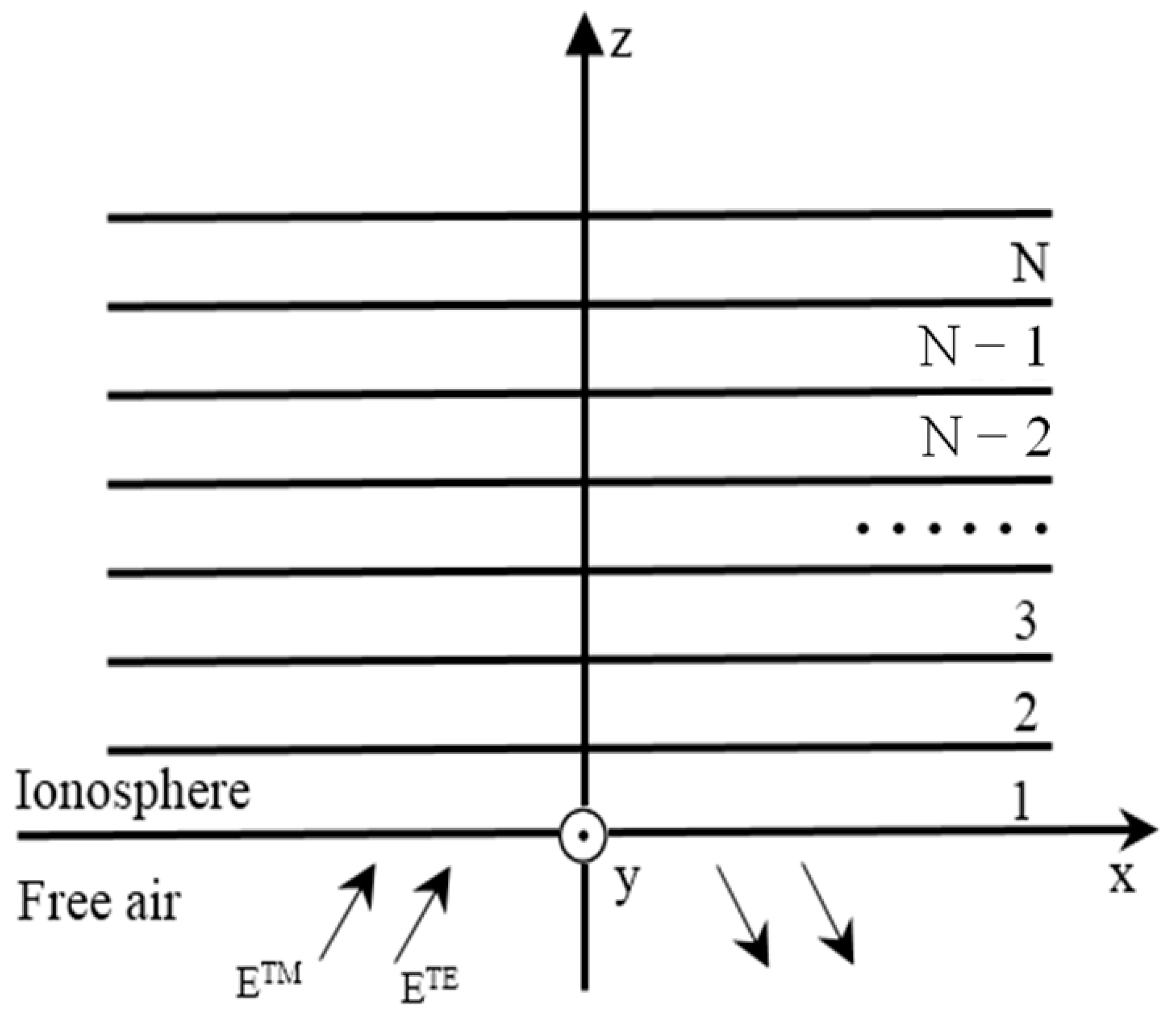
To accurately analyze the electromagnetic properties of the ionosphere, we first establish a horizontally stratified ionospheric model, as depicted in Figure 1. Throughout the height space of the ionosphere, we assume the uniformity of the geomagnetic field. In Figure 1, z is the ground height, and the xoy plane signifies the horizontal reference plane. The ionospheric base lies within this plane, and the entire inhomogeneous anisotropic ionosphere is horizontally partitioned into several layers based on altitude. The height of each layer is substantially smaller than the wavelength, ensuring the uniformity of electron density within each layer. Conforming to this model, the ionosphere can be conceptualized as an assembly of multilayer anisotropic media. Assuming the geomagnetic field’s direction in Figure 1 to be arbitrary, with angles α, β, and γ representing its orientations along the x, y, and z axes, respectively, ETM and ETE represent two polarization forms of the electromagnetic waves, respectively (Figure 1).

Figure 1.
Horizontal multilayer anisotropic structure of the ionospheric model.
The complex dielectric permittivity of the ionosphere is denoted by [19] and can be expressed as follows:
The elements in the matrix are as follows:
where ω is the frequency of the incident wave, ω0 is the plasma frequency, ωT is the magnetic rotation frequency, and υ is the collision frequency. Additionally, H0 is the intensity of the geomagnetic field, N0 is the electron density, me is the electron mass, and e is the charge. The values of N0 and υ can be obtained based on the International Reference Ionosphere (IRI) [2,3,4].
Here,
ω02 = (N0e2)/(meε0), ωT = (μ0eH0)/me
The following sections systematically discuss the proposed model and the transfer matrix applicable to any anisotropic medium, employing the principles of the transfer matrix method. The relative permeability of the ionosphere is 1 [7,8].
3. Transfer Matrix Method
Theoretical Derivation
In our investigation of the anisotropic ionosphere, we investigate the electromagnetic propagation within an anisotropic multilayer structure. The electromagnetic parameters in nonuniform anisotropic multilayer media are represented in the form of tensors, that is, the electromagnetic parameters are a matrix containing nine elements, and the propagation of electromagnetic waves in anisotropic media will exhibit complex scattering phenomena [21]. This complexity poses a challenge to the electromagnetic characteristics of computational structures. To address this complexity, we adopt the concept of transfer matrix and systematically derive the transfer matrix of multilayer structures of arbitrary anisotropic materials through comprehensive analysis and calculation of various anisotropic media, which is used for electromagnetic wave transmission characteristic calculation [22,23]. In fact, the idea of using a layered model and constructing a transfer matrix is an effective way to analyze electromagnetic scattering in nonuniform media. Ref. [24] proposedand tested a ray theory and transfer-matrix-method-based model for a lightning electromagnetic pulse (LEMP) propagating in the Earth–ionosphere waveguide (EIWG). This article applies the above ideas to the precise analysis of short-wave electromagnetic scattering in the nonuniform ionosphere.
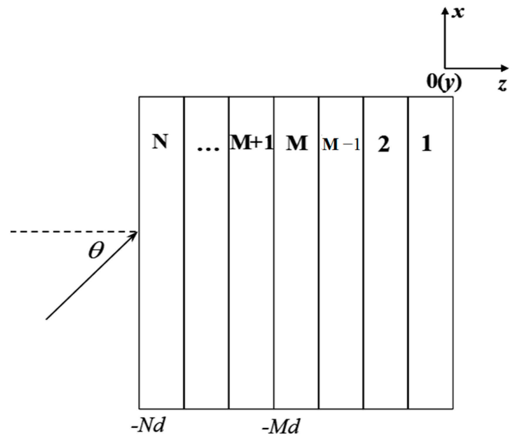
The general structure of anisotropic horizontal-layered multilayer media is depicted in Figure 2. It consists of n layers of dielectric materials, each being a homogeneous anisotropic medium with electromagnetic parameters expressed in tensor form: [εij], [μij] (i, j = 1, 2, 3). These parameters may vary between layers. For simplification, we assume equal thickness (d) for all layers. The electromagnetic wave is obliquely incident at an angle θ, with the incident plane being the xoz plane. The eigen equation of the electromagnetic field in the nth layer material is obtained [25]:
where εij, μij (i,j = 1,2,3) represent the electromagnetic parameters of the layer, and δ = sinθ.
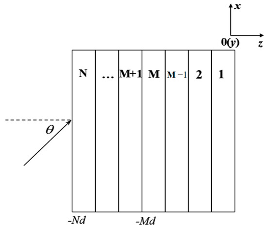
Figure 2.
Anisotropic horizontal-layered multilayer media structure.
Let the eigenvalues and eigenvectors of Equation (4) be γ(M) and W(M) (4 × 4 matrix), respectively, where γ(M) = [γ(M)1, γ(M)2, γ(M)3, γ(M)4], and γ(M)1 and γ(M)2 are greater than 0, while γ(M)3 and γ(M)4 are less than 0. Where γ(M)1 represents the incident type I incident wave, and γ(M)3 represents the type I reflected wave, γ(M)2 represents the type II incident wave, and γ(M)4 represents the type II reflected wave. Electromagnetic waves entering anisotropic media will split into two waves with different polarization forms, namely, ordinary waves and extraordinary waves. In this article, the above waveforms are defined as type I waves and type II waves, respectively [18]. The field distribution in the M-layer region can be expressed as follows:
Here, η = 120π; the elements of the diagonal array X(M) are X(M)(j,j) = exp(k0γ(M)j(z +(M − 1)d)), (j = 1,2,3,4); the elements of the diagonal array G(j,j) = exp(k0(xδ)); and u(M)1,v(M)1 and u(M)2,v(M)2 are the amplitudes of the up and down waves of the TE wave and TM wave in material m, respectively.
Similarly, the field distribution of the (M − 1) layer and (M + 1) layer area can be obtained, establishing the field relationship between the two subinterfaces of layer m:
Q = W(M)·X(M)·W(M)−1·P
The feature vectors in free space are as follows:
T = T(1) × T(2) × … T(N−1) × T(N)
The feature vectors in free space are as follows:
where β = cosθ.
At z = 0, only transmitted waves are present with no reflected waves. Then, the relationship between the free-space field at z = −Nd and the field at z = 0 is as follows:
Here,
We define the following relationships:
The reflection matrix R can be obtained from Equation (8).
The matrix R represents a generalized reflection coefficient encompassing multiple optical reflection processes. This matrix contains four complex elements. R11 is the reflection coefficient of a type I wave reflected into another type I wave; R22 is the reflection coefficient of a type I wave reflected into another type I wave. R12 and R21 are the reflection coefficients of a type I wave reflected into a type II wave and a type II wave reflected into a type I wave, respectively. These coefficients capture the coupling characteristics between type I waves and type II waves.
4. Analysis and Verification of Short-Wave Electromagnetic Scattering in the Heterogeneous Anisotropic Ionosphere
4.1. Effects of Ionospheric Anisotropy on the Highest Frequencies
Short waves are significantly influenced by the high ionosphere (F layer), particularly evident in the critical frequency, also referred to as the maximum reflection frequency. In this section, we establish a model of a uniform sharp boundary F-layer ionosphere and calculate the change in the critical frequency of short waves before and after considering the influence of the geomagnetic field, employing both the traditional method and the proposed method. When a critical frequency radio wave is projected vertically into the ionosphere, the waves that can be reflected back from each layer of the ionosphere (such as the E layer and F layer) have their highest frequencies, which are called the “critical frequencies” (sometimes also known as “cutoff frequencies”) of each layer.
In the traditional method, the critical frequency fc can be expressed as follows:
Nmax is the maximum electron concentration at the ionospheric reflection point, typically situated in the F2 layer. The highest reflected frequency for oblique incident radio waves can be expressed as follows:
where θ0 is the angle of incidence.
Considering the statistical average of the ionospheric electric parameters of the F2 layer in the summer daytime, namely, Nmax = 1 × 10¹² m−3, the collision frequency υ = 103 times/s, with an incidence angle of 30°. Without considering the geomagnetic field, the maximum reflection frequency which is calculated by Equation (14) is 10.3 MHz. Then, introducing the average value of the geomagnetic field 5 × 10⁻⁵ T (unit) and assuming the F2 layer exhibits uniform electromagnetic anisotropy, its equivalent dielectric constant is calculated according to Section 2. The algorithm proposed in this paper is then employed to calculate the maximum reflection frequency, yielding approximately 9.6 MHz. Figure 3 illustrates the comparison curve of the aforementioned calculations.
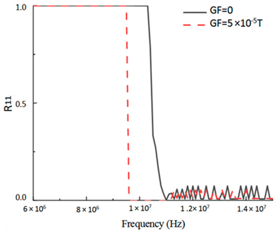
Figure 3.
R11 curve with frequency before and after the introduction of the geomagnetic field.
As illustrated in Figure 3, for only an isotropic homogeneous high ionosphere, the critical frequency calculated by the transmission matrix method aligns closely with the traditional method. This verifies the method’s applicability to a certain extent within the short-wave frequency band. Secondly, in the uniform sharp boundary F-layer ionospheric model, ionospheric anisotropy primarily influences the critical frequency. When factoring in the geomagnetic field, the maximum reflection frequency decreases by approximately 0.8 MHz. Thus, ionospheric anisotropy notably influences short waves, and the modulus of the reflection system tends to 1 before the frequency reaches the maximum reflection frequency, attributable to the low collision frequency in the F layer and minimal absorption loss. This leads to the conclusion that the propagation characteristics of short waves in the ionosphere cannot be fully described solely by considering the high ionosphere but should also fully consider the scattering and absorption effects caused by the anisotropy of lower ionospheres such as the D and E layers under the influence of the geomagnetic field.
4.2. Computational Comparison of Simple Ionospheric Stratification
As shown in Figure 4, for the entire ionosphere, the modulus of the reflection system does not indefinitely approach 1. However, the maximum reflection frequency undergoes minimal change. This suggests that different regions of the ionosphere exert varying influences on short-wave propagation, with D and E layers primarily affecting absorption loss, and the F layer predominantly influencing the maximum reflection frequency [24]. Simultaneously, after establishing the complete ionosphere, the geomagnetic field not only affects the maximum reflection frequency but also the amplitude of the reflection coefficient, signifying absorption loss. Consequently, when considering anisotropy, the absorption loss of short waves propagating in the ionosphere increases, leading to a decrease in the maximum reflective frequency. The slight fluctuations at the graph’s end resultfrom matrix calculations, with numerical jitter occasionally occurring as the calculation approaches 0, introducing a burr phenomenon in the graph.
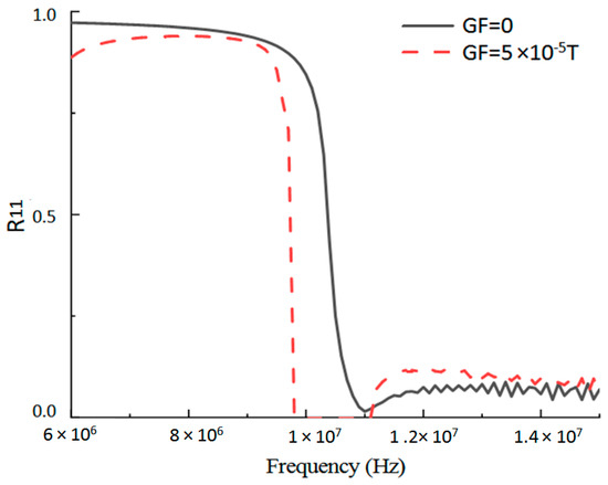
Figure 4.
R11 curve with frequency before and after the introduction of the geomagnetic field.
4.3. Accurate Calculation of Electromagnetic Scattering in the Complex Anisotropic Ionosphere
To analyze the precise scattering characteristics of short waves in the anisotropic ionosphere model, a comprehensive anisotropic ionosphere model was established, as described in Section 2. The dielectric constants of each layer are derived from formulae, and the electrical parameters of each layer are obtained from IRI-2016 [25], utilizing ionospheric data within the height range of 60–400 km. By varying electron density, incident angle, geomagnetic inclination, and radio-wave propagation direction, changes in the inverse transmission coefficient are observed. The scattering law of short waves in the anisotropic ionosphere is summarized, elucidating the influence of the complex anisotropic ionosphere on short-wave propagation.
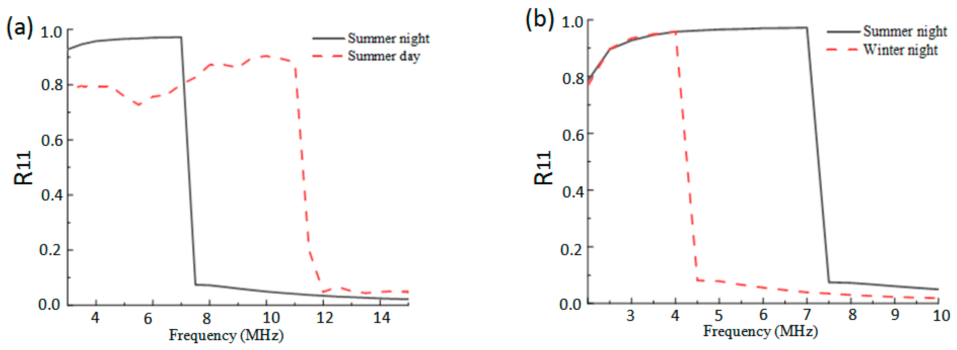
For a specific location, the ionospheric electron density for four typical time periods at the height of 60–400 km—summer day, summer night, winter day, and winter night—is obtained for a detailed analysis and comparison of ionospheric seasonality and diurnal variability. Figure 5a demonstrates a significant difference in electron concentration between the daytime and nighttime, with the peak value differing by nearlyan order of magnitude. Figure 5b illustrates that the peak electron concentration in summer is slightly higher than in winter, and the nocturnal peak is higher than the daytime peak.
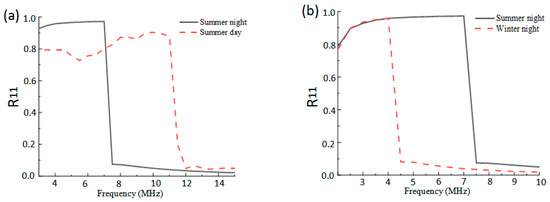
Figure 5.
(a) R11 curve with frequency at night and during the day; (b) R11 curvewith frequency in summer and winter.
Considering the aforementioned electron-concentration distribution as the electrical parameter for the anisotropic ionospheric model, the reflection coefficient at this time is calculated. The collision frequency is considered as the statistical value for each layer, and the geomagnetic field intensity is set at 5 × 10⁻⁵ T. The changes in the reflection coefficient between night and day are compared. As illustrated in Figure 5a, the critical frequency during the day is approximately 5.5 MHz higher than that at night, attributed to the higher electron density during daylight hours. The modulus value of the reflection system at the critical frequency during the night is roughly 0.1 higher than in the daytime, indicating increased ionospheric activity and absorption loss during the daytime compared to nighttime. Comparing the variation in reflection coefficient between summer and winter, Figure 5b indicates that the critical frequency in the ionosphere during summer is approximately 3.5 MHz higher than in winter. The amplitude of the reflection coefficient at the critical frequency for both seasons is almost identical. This can be attributed to the slightly higher electron density in summer, although the disparity in ionospheric ion activity is not as pronounced as in the day–night variations. In summary, seasonal and diurnal fluctuations in the ionosphere significantly influence short-wave propagation, with summer and daytime exhibiting higher propagation effects. Diurnal variation has a more pronounced impact than seasonal variation.
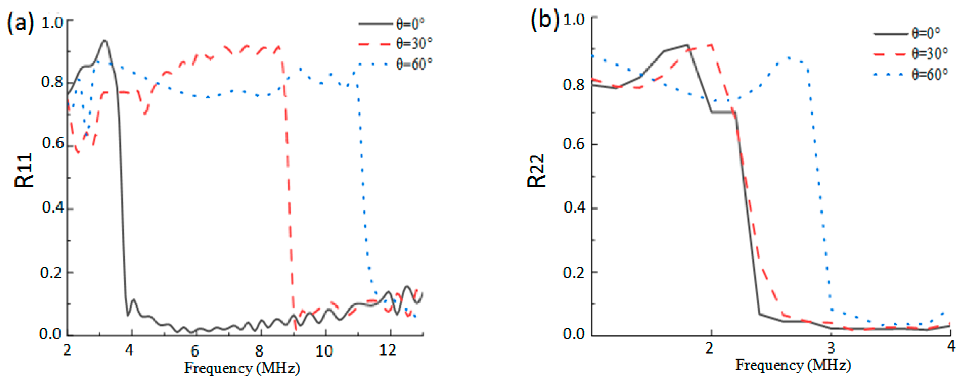
The influence of the incident angle on the back transmission coefficient was analyzed at incidence angles of 0°, 30°, and 60°, respectively. Figure 6 illustrates that with an increase in the incident angle, the critical frequency rises, and the amplitude of the reflection coefficient at the critical frequency slightly decreases. In the anisotropic ionospheric model, the maximum reflection frequency increases substantially with changes in the incident angle, leading to a corresponding increase in ionospheric absorption loss.
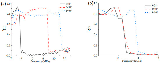
Figure 6.
(a) R11 curve with frequency at incidence angles of 0°, 30°, and 60°; (b) R22 curve with frequency at incidence angles of 0°, 30°, and 60°.
DIP, defined as the angle between the geomagnetic field and the vertical direction (complementary to the geomagnetic inclination), is analyzed for its impact on the reflection coefficient. Figure 7 illustrates that the maximum reflection frequency of horizontally polarized waves increases with the complementary angle of geomagnetic inclination, while the trend is opposite for vertically polarized waves. In equatorial regions, the ionospheric anisotropy caused by the geomagnetic field has the least influence on short-wave propagation, while polar regions experience the most notable influence.
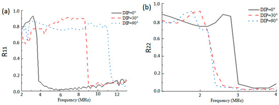
Figure 7.
(a) R11 curve with DIP when DIP is 0°, 60°, and 90°; (b) R22 curve with DIP when DIP is 0°, 60°, and 90°.
The angle denoted as φ represents the inclination between the horizontal component of the geomagnetic field and the direction of propagation. Specifically, φ equals 90° during eastward propagation and 0° during northward propagation. As illustrated in Figure 8, for horizontally polarized waves, the impact of anisotropy on north–south propagation is less pronounced than on east–west propagation. Conversely, vertically polarized waves exhibit the opposite trend, with a more discernible difference. When propagating north–south, the electric field and magnetic field directions are approximately parallel, resulting in a Lorentz force close to zero on free electrons. Nevertheless, empirical observations based on our long-term short-wave communication-performance tracking reveal instances where east–west propagation outperforms north–south propagation due to greater ionospheric variation in the north–south direction. It is noteworthy, however, that the ionospheric model proposed in this paper adopts horizontal stratification, potentially overlooking the horizontal nonuniformity of the ionosphere, thereby introducing limitations. Consequently, when selecting the propagation direction in practical communication, one should consider not only the influence of the geomagnetic field but also the nonuniformity of the ionosphere across the horizontal span of the link.
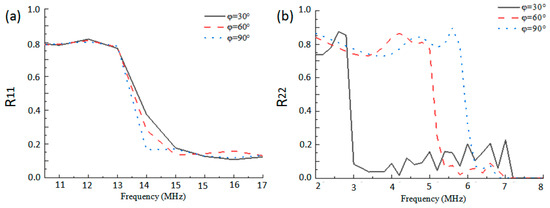
Figure 8.
(a) R11 curve with frequency when is 30°, 60°, and 90°; (b) R22 curve with frequency when is 30°, 60°, and 90°.
The burr phenomenon observed in the reflection coefficient curve with frequency in this section is attributed to numerical overflow and flutter phenomena generated by the computer when the matrix cascade calculation becomes too extensive or when the results approach infinity and zero.
In conclusion, considering nonuniform anisotropy, the precise scattering characteristics of short-wave propagation in the ionosphere were analyzed. Under the influence of geomagnetic storms or solar activities, the electron density of the ionosphere will change significantly with time and season [26,27,28,29]. Based on the ionospheric statistical data of IRI, the daily variation, seasonal variation, different incidence angles, different latitudes and different propagation directions, and other factors have been carefully studied, and a series of propagation laws have been obtained. These findings have important reference value for improving the practicability of short-wave communication
5. Comparison Validation
To ascertain the precision of the established anisotropic ionospheric scattering model and its corresponding algorithm, this chapter selects two communication links during an extended voyage as the context. Measured data serve as the benchmark for predicting the median value of sky-wave field intensity. The algorithm’s field-intensity predictions are then compared with those based on the ITU-R P.533 statistical model.
5.1. Communication Link
The transmitting (red point) and receiving (blue point) stationsfor the measured data are depicted in Figure 9.
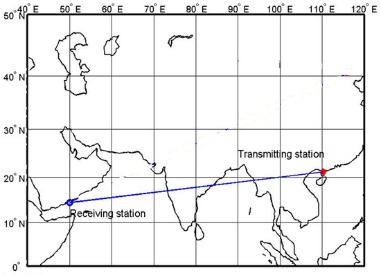
Figure 9.
Probe site distribution.
The data collection period spanned from 1 May 2015 to 30 June 2015, yielding over 1190 valid data points as shown in Figure 10. The detection data comprise frequency–height maps and spectral maps. After processing, maximum observation frequency (MOF), maximum usable frequency (MUF), optimum working frequency (OWF), and height probable frequency (HPF) can be derived.
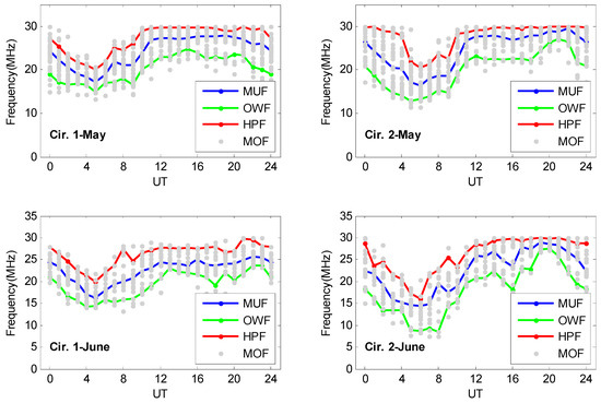
Figure 10.
Data source diagram of the communication link.
In reality, there are multiple modes of long-distance short-wave propagation, including both the multihop mode in the F2 layer and the multihop mode in the E layer. According to ITU-R P.533 [30,31], during long-distance transmission, the field-strength attenuation of the E-layer multihop mode is significant, and its contribution to the field strength of the receiving point is very low. As the short-wave propagation distance in this case is about 7100 km, the calculation process is simplified while ensuring calculation accuracy. Based on ITU-R P.533 [30], we only choose the F2-layer multihop mode and ignore the E-layer multihop mode. Subsequently, we analyze the field strength of the F2 layer in the 1–6 hop mode. Since the receiving station employs automatic gain control technology for HF communication, adjusting gain based on signal strength, received field strength does not precisely represent the actual environmental field strength. Thus, we use the field strength obtained through MOF inversion calculation as the benchmark, representing the “true field strength” closely aligned with the objective environment. The field strength is calculated through the MOF inversion and deduction method outlined in ITU-R P.533 [30].
5.2. Median Field-Strength Prediction Based on the Statistical Model
This study employed the sky-wave field-intensity prediction method based on the reference statistical model to forecast the median value for the link during the same period. The approach aligns with the widely utilized recommendation ITU-R P.533-12 [25]. Given the link’s distance of approximately 7100 km, the formula for median field strength for paths exceeding 7000 km is as follows:
where
fH is the average of the electron rotation frequencies determined at the two control points, fM is determined by the MUF, and fL is determined by the LUF.
F is the transmission frequency (Mhz), Pt is the transmitter power(dB), Gt is the transmitting antenna power(dB), and Lb is the basic transmission loss of the path, expressed by the following formula:
where P′ denotes the virtual slant distance (km), Lm denotes the absorption loss (dB), denotes the loss “above MUF”, Lg denotes the sum of the ground reflection loss, Lh denotes the factor that accounts for the auroral and other signal losses, and Lz accounts for other effects of sky-wave propagation.
5.3. Field-Strength Calculation Based on the Anisotropic Backscattering Model
In this paper, the distance of the link is about 7100 km, and the majority of energy is reflected and transmitted within the F2 layer, primarily in the 1–6 hopmode [31].
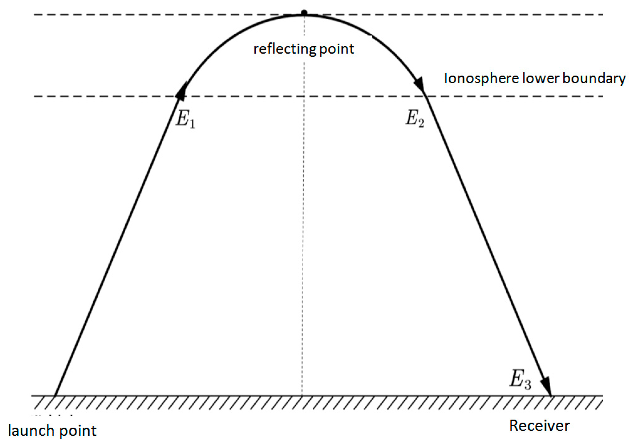
For a one-hop scenario, the propagation mode of the radio wave in the scattering model is depicted in Figure 11. The radiation-power density in the maximum radiation direction of the antenna is calculated as follows:
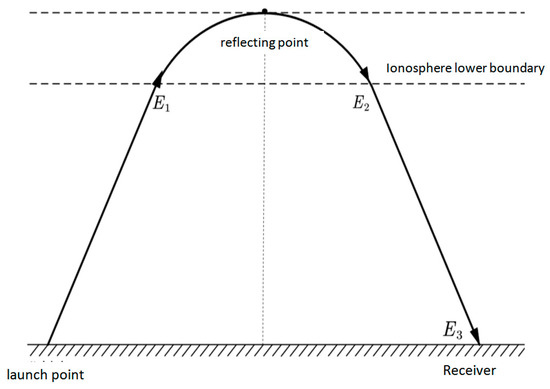
Figure 11.
Scattering model of the wave propagation path.
Combined with the direction function f(θ,), where r denotes the free-space propagation distance from the transmitting point to the ionospheric incident point, obtained based on the propagation mode, ionospheric reflection point height, and communication distance, yields the radiation field intensity E1 at the ionospheric incident point:
As discussed in Section 4, the ionosphere in the scattering model is a horizontally stratified model. Thus, we can assume the propagation trajectory of the radio waves in the ionosphere forms a symmetric parabola. In this scenario, the highest point of the parabola serves as the control point, and the ionosphere is modeled as a horizontally stratified anisotropic ionosphere. Electrical parameters are derived from the Chinese Reference Ionosphere (CRI) [26], with horizontally polarized waves as the focus. By calculating the reflection coefficient R11 at the control point, the radiation field intensity E2 of the radio wave at the ionospheric exit point can be expressed as follows:
After the ionospheric reflection, the radio wave reaches the receiving point through a period of free-space loss and additional system loss, eventually yielding the receiving point field strength E3. Free-space propagation loss is denoted as L0, and extra system loss is denoted as LP, where
Assuming the radio wave’s propagation path is generally symmetrical, r is the propagation distance in free space from the ionospheric exit point to the receiving point and from the transmitting point to the incident point in the ionosphere, which can align with the distance variable in Equation (19). Lp is calculated according to ITU-R recommendation P.533-12 [30]. In the case of multiple hops, parameters such as the incident angle and free-space transmission distance must be recalculated for each radio-wave propagation path. Subsequently, the field-strength results for 1 to 6 hops are calculated and comprehensively accumulated to obtain the predicted median field-strength value.
In summary, the scattering model calculation method integrates semiempirical formulae and the reflection coefficient calculated by the anisotropic ionospheric model. When compared to the statistical model, the ionospheric model, accounting for anisotropy and high inhomogeneity, is expected to yield more accurate results.
5.4. Comparative Analysis
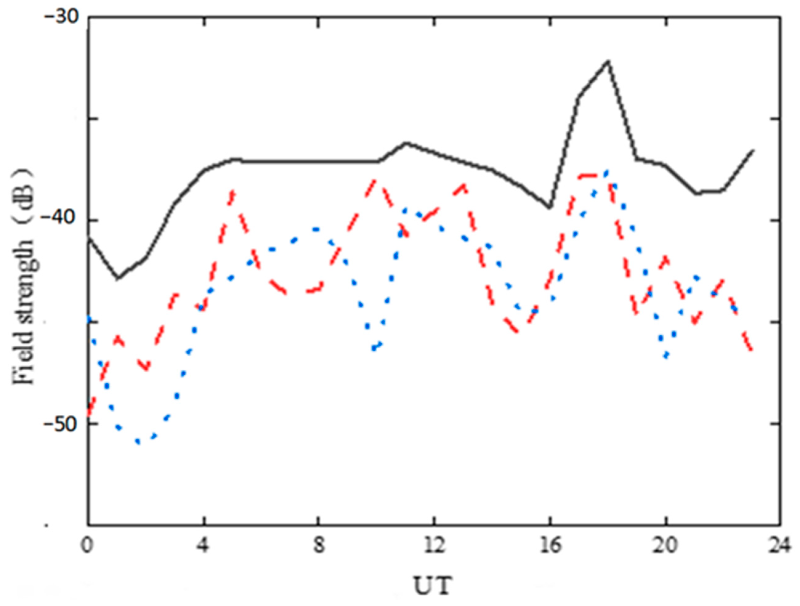
Figure 12 and Figure 13 illustrate the comparison between the link field-strength inversion and prediction calculations conducted in May and June, respectively. The prediction calculation input conditions are consistent with the measurement conditions. The blue dashed line represents the MOF inversion field-strength results from the observation data, the red dashed line represents the calculated field-strength results from the ionospheric scattering model, and the black solid line represents the calculated field-strength results obtained using the statistical reference model.
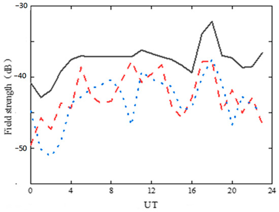
Figure 12.
Field-strength calculation results of the first link in May.
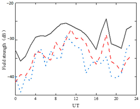
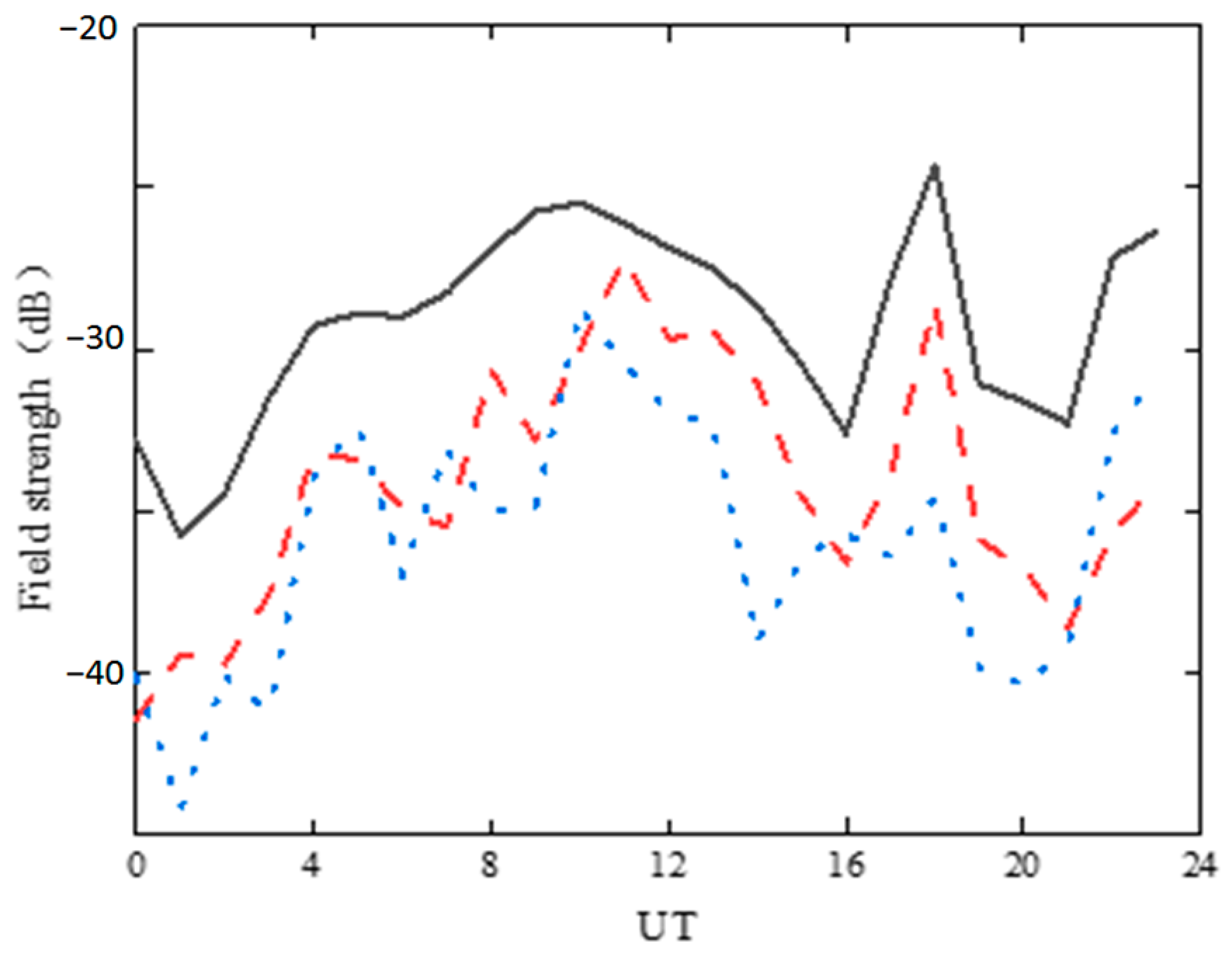
Figure 13.
Field-strength calculation results of the first link in June.
Figure 12 and Figure 13 show that whether using the statistical reference model or the scattering model in this paper, the calculated results have the same trend as the actual values. Therefore, the above two models have good reference significance in short-wave communication prediction. In addition, compared with the statistical reference model, the calculated values of the scattering model in this paper are closer to the actual values, indicating that the model in this paper has better calculation accuracy.
In conclusion, considering the ionospheric anisotropy, the scattering model exhibits commendable accuracy in predicting the field intensity of long-distance short-wave propagation. The model closely approximates the actual ionosphere, holding significant reference value for guiding short-wave communication.
In the establishment of ionospheric models, commonly used ionospheric models were analyzed, and a horizontal-layered model was selected to overcome the nonuniformity of ionospheric height. Only considering the model’s adaptation to typical scenarios, but not fully considering the horizontal nonuniformity of the ionosphere, errors may occur in ionospheres with strong horizontal nonuniformity. Further optimization of algorithms and models is needed to improve the accuracy of the propagation of radio waves in the ionosphere.
6. Summary
This study assessed the influence of ionospheric anisotropy on radio-wave propagation, considering three focal areas: model construction algorithm derivation, scattering characteristic computation, and field-intensity prognosis. First, the ionospheric structure was analyzed, followed by the assessment of the pros and cons of various models. Subsequently, an anisotropic ionosphere model was established based on calculations. In addition, the scattering characteristics and propagation principles of very-long-wave and short-wave military communication bands within the anisotropic ionosphere were examined. Finally, the anisotropic ionospheric scattering model was used to predict and validate the median value of sky-wave field intensity. The findings using the proposed method were closer to the measured data than those using the statistical model, thereby confirming the accuracy of the anisotropic ionosphere model. In field-strength prediction, the average error of the scattering model proposed in this article is generally smaller than that of the statistical model, which has better accuracy, proving that its field-strength calculation method is superior to the statistical method. Due to limitations, we still use ionospheric statistical data provided by IRI for calculation in this model. Of course, changes in geomagnetic activity and solar radiation can lead to anisotropic fluctuations. In order to obtain more accurate calculation results, the data in this model can be replaced with real-time observation data. All calculations in this article are based on MATLAB. Although the method presented in this article is complex in mathematical derivation, it is very easy and fast for MATLAB R2013b, which has strong matrix computing capabilities, to obtain results. Real-time calculations can be performed using ordinary computers. Therefore, the construction of the ionospheric scattering model field-strength prediction method based on this article can provide good support for the evaluation of long-distance short-wave communication efficiency or field-strength prediction.
Author Contributions
Conceptualization, Z.Z. and L.Z.; methodology, Z.Z., J.S. and L.Z.; software, Z.Z. and J.S.; validation, L.Z. and J.S.; formal analysis, Z.Z. and L.Z.; writing—original draft preparation, Z.Z. and J.S.; writing—review and editing, L.Z. and H.F.; supervision, H.F. and S.J. All authors have read and agreed to the published version of the manuscript.
Funding
This research received no external funding.
Informed Consent Statement
Not applicable.
Data Availability Statement
The data presented in this study are available on request from the corresponding author. The data are not publicly available due to privacy.
Conflicts of Interest
The authors declare no conflicts of interest.
References
- Bertel, L.; Guyader, P.; Lassudrie, D.; Uchesne, P. Multiple-frequency Doppler sounding of the ionosphere: Theory and experimental comparison with incoherent scatter results. Radio Sci. 1984, 19, 879–890. [Google Scholar] [CrossRef]
- Helliwell, R.A. Whistlers and Related Ionospheric Phenomena; Stanford University Press: Stamford, CT, USA, 1965. [Google Scholar]
- Cohen, M.B.; Gross, N.C.; Higginson-Rollins, M.A.; Marshall, R.A.; Gokowski, M.; Liles, W.; Rodriguez, D.; Rockway, J. The Lower Ionospheric VLF/LF Response to the 2017 Great American Solar Eclipse Observed Across the Continent. Geophys. Res. Lett. 2018, 45, 3348–3355. [Google Scholar] [CrossRef]
- Kelso, J.M. Ray Tracing in the ionosphere. Radio Sci. 1968, 3, 1–12. [Google Scholar] [CrossRef]
- Haselgrove, J. Ray theory and a new method of raytracing. In Physics in the Ionosphere; London Press: London, UK, 1965. [Google Scholar]
- Jones, R.M. A three-dimensional ray-tracing computer program (digest of ESSA technical report, ITSA no. 17). Radio Sci. 1968, 3, 93–94. [Google Scholar] [CrossRef]
- Croft, T.A.; Hoogasian, H. Exact ray calculations in a quasi-parabolic ionosphere with no magnetic field. Radio Sci. 1968, 3, 69–74. [Google Scholar] [CrossRef]
- Dyson, P.L.; Bennett, J.A. A model of the vertical distribution of the electron concentration in the ionosphere and its application to oblique propagation studies. J. Atmos. Terr. Phys. 1988, 50, 251–262. [Google Scholar] [CrossRef]
- Norman, R.J.; Cannon, P.S. A two-dimensional analytic ray tracing technique accommodating horizontal gradients. Radio Sci. 1997, 32, 387–396. [Google Scholar] [CrossRef]
- Davies, K.; Rush, C.M. High-frequency ray paths in ionospheric layers with horizontal gradients. Radio Sci. 1985, 20, 95–110. [Google Scholar] [CrossRef]
- Coleman, C.J. On the simulation of backscatter ionograms. J. Atmos. Sol. Terr. Phys. 1997, 59, 2089–2099. [Google Scholar] [CrossRef]
- Coleman, C.J. A ray tracing formulation and its application to some problems in over-the-horizon radar. Radio Sci. 1998, 33, 1187–1197. [Google Scholar] [CrossRef]
- Xie, S.G.; Zhao, Z.Y. A new ray-tracing method-three zoning treatment. Chin. J. Radio Sci. 2001, 16, 222–226. [Google Scholar]
- Muldrew, D. An ionospheric ray-tracing technique and its application to a problem in a long-distance radio propagation. IRE Trans. Antennas Propag. 1959, 7, 393–396. [Google Scholar] [CrossRef]
- Hopkins, H.G.; Reynolds, L.G. An experimental investigation of short-distance ionospheric propagation at low and very low frequencies. Proc. IEE Part III Radio Commun. Eng. 1954, 69, 21–34. [Google Scholar]
- Song, H.; Qing, H.; Zou, X. A parallel optimization 3D numerical ray-tracing method for the fast and accurate simulation of disturbed oblique ionogram. Adv. Space Res. 2022, 70, 2894–2899. [Google Scholar] [CrossRef]
- Yaogai, H.; Zhengyu, Z.; Yuannong, Z. Ionospheric disturbances produced by chemical releases and the resultant effects on short-wave. J. Geophys. Res. 2011, 16, A07307. [Google Scholar]
- Liu, W.; Peinan, J.; Shikai, W.; Junjiang, W. A fast ray tracing algorithm in the ionosphere. Chin. J. Radio Sci. 2008, 01, 41–48. [Google Scholar]
- Jiangquan, C.; Yuhong, Y.; Xin, G.; Song, L. Simulation of shortwave 3D ray tracing with geomagnetic field. Comput. Eng. Des. 2012, 33, 300. [Google Scholar]
- Krasnov, V.M.; Kuleshov, Y.V.; Koristin, A.A.; Drobzheva, Y.V. Influence of the geomagnetic field on absorption of radiowaves. J. Atmos. Sol.-Terr. Phys. 2021, 227, 105806. [Google Scholar]
- Pan, W.Y.; Li, K. Propagation of SLF/ELF Electromagnetic Waves; Springer: Berlin/Heidelberg, Germany, 2014. [Google Scholar]
- Wang, J. Observation and analysis of phase cycle slipping of VLF signals. Chin. J. Radio Sci. 2006, 21, 628–631. [Google Scholar]
- Fu, H.; Zhang, Z.; Ju, J. Calculation of shortwave propagation in anisotropic ionosphere by transfer matrix method. In Proceedings of the 2021 IEEE 5th Advanced Information Technology, Electronic and Automation Control Conference (IAEAC), Chongqing, China, 12–14 March 2021; IEEE: Piscataway, NJ, USA, 2021; Volume 5, pp. 1983–1986. [Google Scholar]
- Qin, Z.; Chen, M.; Zhu, B.; Du, Y.P. An improved ray theory and transfer matrix method-based model for lightning electromagnetic pulses propagating in Earth-ionosphere waveguide and its applications. J. Geophys. Res. Atmos. 2017, 122, 712–727. [Google Scholar] [CrossRef]
- Zhao, L.; Zuo, Y.; Feng, Y.J. Electromagnetic Wave Reflection of Anisotropic Layered Media with a Metallic Substrate. Chin. J. Radio Sci. 2009, 24, 5. [Google Scholar]
- Ding, Z.H.; Dai, L.D.; Yang, S.; Miao, J.S.; Wu, J. Preliminary analysis of diurnal variation characteristics of electron density in the E-F valley region of the ionosphere using incoherent scattering radar in Qujing. Chin. J. Radio Sci. 2022, 37, 357. [Google Scholar]
- Gwal, A.K.; Choudhary, S.; Chaurasia, H. Chapter 15—Space Weather Phenomenon of Polar Ionosphere Over the Arctic Region. In Understanding Present and Past Arctic Environments; Elsevier: Amsterdam, The Netherlands, 2021; pp. 325–341. [Google Scholar]
- Romero-Hernandez, E.; Denardini, C.M.; Jonah, O.F.; Essien, P.; Picanço, G.A.S.; Nogueira, P.A.B.; Rodriguez-Martinez, M.; Resende, L.C.A.; de la Luz, V.; Aguilar-Rodriguez, E.; et al. Nighttime Ionospheric TEC Study Over Latin America During Moderate and High Solar Activity. JGR Space Phys. 2020, 125, e2020JA028210. [Google Scholar] [CrossRef]
- Lopez-Urias, C.; Vazquez-Becerra, G.E.; Nayak, K.; Lopez-Montes, R. Analysis of Ionospheric Disturbances during X-Class Solar Flares (2021–2022) Using GNSS Data and Wavelet Analysis. Remote Sens. 2023, 15, 4626. [Google Scholar] [CrossRef]
- International Telecommunication Union. Method for the Prediction of the Performance of HF Circuits; ITU-RP.533; International Telecommunication Union: Geneva, Switzerland, 2007. [Google Scholar]
- Yan, Z.W.; Wang, G.; Tian, G.L.; Li, W.M.; Su, D.L.; Rahman, T. Errata to “The HF Channel EM Parameters Estimation Under a Complex Environment Using the Modified IRI and IGRF Model”. IEEE Trans. Antennas Propag. 2011, 59, 2448. [Google Scholar] [CrossRef]


Disclaimer/Publisher’s Note: The statements, opinions and data contained in all publications are solely those of the individual author(s) and contributor(s) and not of MDPI and/or the editor(s). MDPI and/or the editor(s) disclaim responsibility for any injury to people or property resulting from any ideas, methods, instructions or products referred to in the content. |
© 2024 by the authors. Licensee MDPI, Basel, Switzerland. This article is an open access article distributed under the terms and conditions of the Creative Commons Attribution (CC BY) license (https://creativecommons.org/licenses/by/4.0/).