Analytical Review of Wind Assessment Tools for Urban Wind Turbine Applications

Abstract

Due to the complex nature of the built environment, urban wind flow is unpredictable and characterised by high levels of turbulence and low mean wind speed. Yet, there is a potential for harnessing urban wind power by carefully integrating wind turbines within the built environment at the optimum locations. This requires a thorough investigation of wind resources to use the suitable wind turbine technology at the correct location—thus, the need for an accurate assessment of wind resources at the proposed site. This paper reviews the commonly used wind assessment tools for the urban wind flow to identify the optimum tool to be used prior to integrating wind turbines in urban areas. In situ measurements, wind tunnel tests, and CFD simulations are analysed and reviewed through their advantages and disadvantages in assessing urban wind flows. The literature shows that CFD simulations are favoured over other most commonly used tools because the tool is relatively easier to use, more efficient in comparing alternative design solutions, and can effectively communicate data visually. The paper concludes with recommendations on best practice guidelines for using CFD simulation in assessing the wind flow within the built environment and emphasises the importance of validating CFD simulation results by other available tools to avoid any associated uncertainties.

1. Introduction

Urban wind turbines have a high potential for in situ power generation since the power transmission losses are significantly reduced due to using the power where it is generated [1]. They can contribute to a more sustainable built environment by making buildings closer to being self-sufficient in terms of energy; however, the main challenge lies in the uncertainty associated with integrating wind turbines within the built environment [2]. This uncertainty stems from the poor performance of urban wind turbines due to the unpredictable nature of wind within the built environment, which is characterised by high turbulence and a low mean wind speed [3,4].

However, it is evident that assessing the wind resources at a particular urban site could inform the design team about the optimum mounting/integration locations of wind turbines. Moreover, it could take advantage of the accelerating effect, which happens when wind collides with an obstacle [5,6]. Assessing the wind condition at a particular site will help identify specific locations where the wind flow is less turbulent and the mean wind velocity is higher. Mounting the wind turbines in these locations will result in a significant increase in the energy yield [7,8].

Accordingly, understanding the wind flow at the mounting location plays an important role in estimating the performance of the proposed wind turbine. The energy yield will depend on factors such as local wind flow conditions, including urban settings, surface cover, and vegetation [9,10]. In addition to local wind flow conditions, there are other factors affecting the successful integration of wind turbines, and these factors include the geographical distribution of wind speeds, characteristic parameters of the wind, topography, and measurement of the mean wind speed [11]. With the aid of Geographic Information Systems (GIS), informed decisions about optimum mounting locations could be reached [12]. Moreover, the emergence of multiple artificial intelligence (AI) applications and machine learning (ML) techniques increases confidence in predicting urban wind flows [13]. In a recent investigation, comparing computational fluid dynamics (CFD) simulation of the pedestrian level wind speed to the results of an ML-based tool using an image similarity assessment method, there was significant agreement between both tools [14]. GIS, AI, and ML could be implemented in conjunction with the most commonly used urban wind assessment tools for more accurate results.

A variety of tools are available for assessing the wind flow within the built environment, with the most common tools being in situ measurements, wind tunnel tests, and CFD simulations [15]. This paper analyses and reviews these tools to identify the optimum tool to be used in assessing urban wind flow. This was carried out by reviewing the pros and cons of each wind assessment tool for the purpose of integrating wind turbines in urban areas.

Accordingly, this article consists of three main sections: (a) understanding wind resources at the installation site considering the macro- and microscale wind conditions; (b) investigation of the most commonly used urban wind assessment tools for studying the wind flow within the built environment, discussing pros and cons of each wind assessment tool to identify areas of application; And (c) in-depth investigation of the proposed urban wind assessment tool with a focus on how to use the tool for obtaining reliable results. The paper concludes with a set of guidelines for using the recommended tool to yield reliable results when studying wind flow in urban areas.

2. Estimation of Wind Resources

Wind resources in any specific location are determined by macroscale and mesoscale wind conditions. As for urban areas, the microscale wind conditions are the main factor affecting wind resources. This is strongly dependant on the geometry of the buildings as well as the urban setting. Local weather stations can provide reliable information about macroscale and mesoscale conditions. However, they cannot provide more detailed data on microscale wind conditions as this has to be collected using specific wind assessment tools. Early investigation of the microscale conditions can affect the design geometry to utilise the local wind for wind power generation, passive cooling, and wind load analysis [16,17].

The main factor affecting the feasibility of integrating wind turbines in urban areas is wind velocity. However, turbulence, which occurs due to the interaction between wind and obstacles in the form of buildings, also affects the energy yield from the integrated wind turbines. Areas with high levels of turbulence should be avoided when considering urban wind turbine installations. High levels of turbulence will result in a reduction in the power output from the wind turbine. To identify areas of high mean wind velocity and low levels of turbulence, wind assessment tools are used to inform the decisions of the optimum mounting/integration locations of wind turbines within the built environment [6].

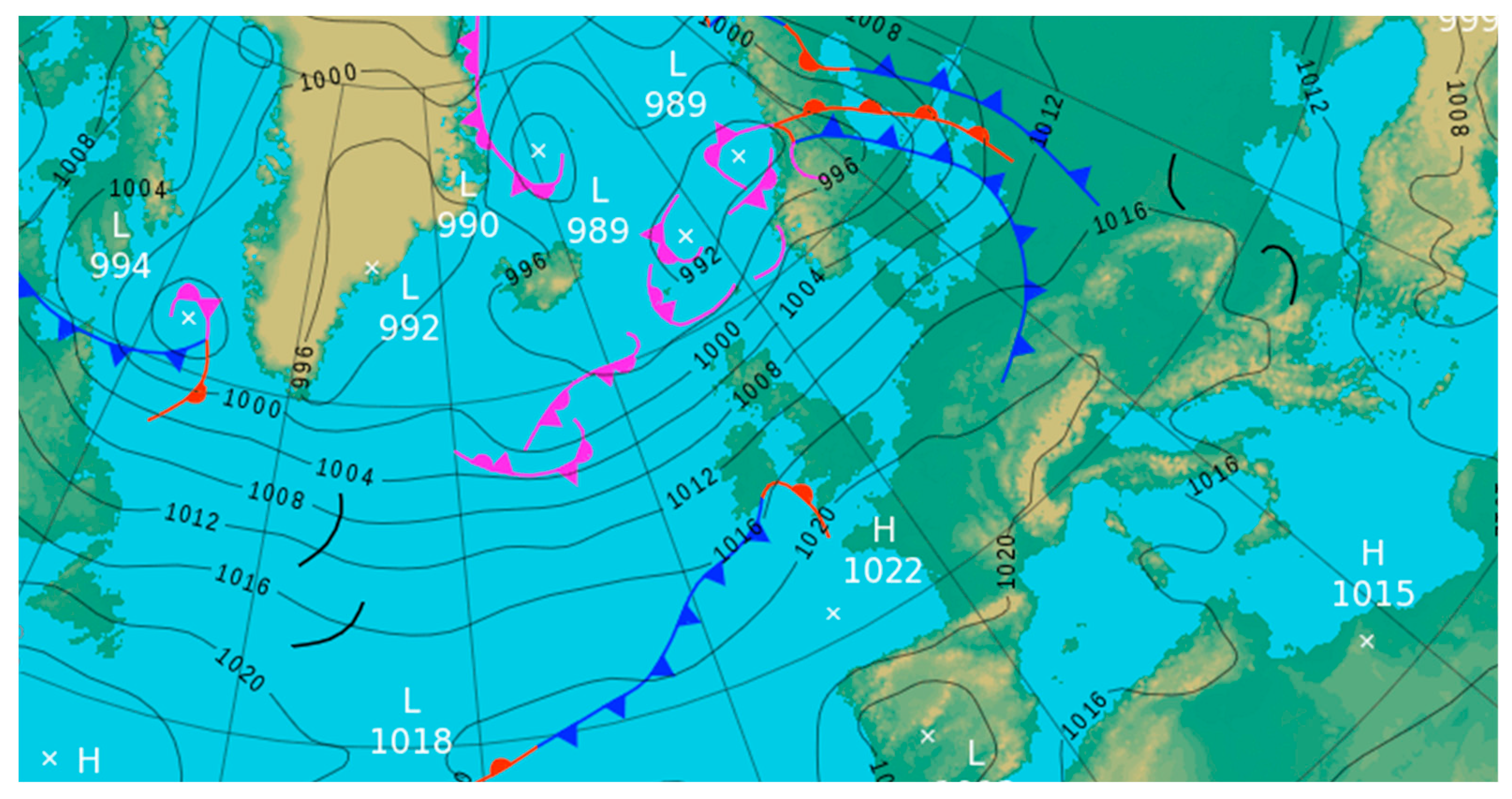
2.1. Macroscale Wind Conditions

Different geographic locations have different climates and wind conditions. The movement of air (wind) is governed by the natural phenomenon of differential temperature between the poles and the equator. The temperature difference results in areas of different pressure values, which causes the air to flow from the areas of high pressure to areas of low pressure, creating air currents, commonly known as the prevailing wind. As seen in Figure 1, isobars represent areas of different air pressure values [18,19,20]. At higher altitudes ranging between one thousand and two thousand meters, the earth’s rotation as well as the curvature of the earth’s surface affects air movement. These forces are ineffective in the atmospheric boundary layer where the frictional forces and drag forces are more prominent at the surface [21].

Global and regional jet streams are natural phenomena resulting from air movement because of temperature differences. The regional phenomenon is determined by orographic conditions, e.g., the surface structure of the area, and by global phenomena. The wind conditions in this area, known as the boundary layer, are influenced by the energy transferred from the undisturbed high-energy stream of the geostrophic wind to the layers below as well as by regional conditions. Turbulence is found near the ground due to the increased roughness [22,23].

These phenomena affect the three main factors in assessing wind energy resources: The first is the mean wind speed per annum, which is dependent on the terrain roughness the wind passes by to reach the studied location and the prevailing wind at a specific location. The second is the wind speed distribution profile, which is the frequency of different wind speeds throughout the year. This factor is necessary for determining the power available in the wind since the energy available in the wind is directly proportional to the cube of the wind speed. The third is the wind direction, which is of paramount importance when thinking of wind power generation in urban areas.

If the type of integration is building-augmented wind turbines, the whole building will be oriented towards the prevailing wind direction to collect the maximum amount of wind since the yawing system of the turbine will not be possible in this scenario. In the case of roof-mounted wind turbines or building-integrated wind turbines, the yawing system could be operational, and the turbine could yaw to face the prevailing wind [24].

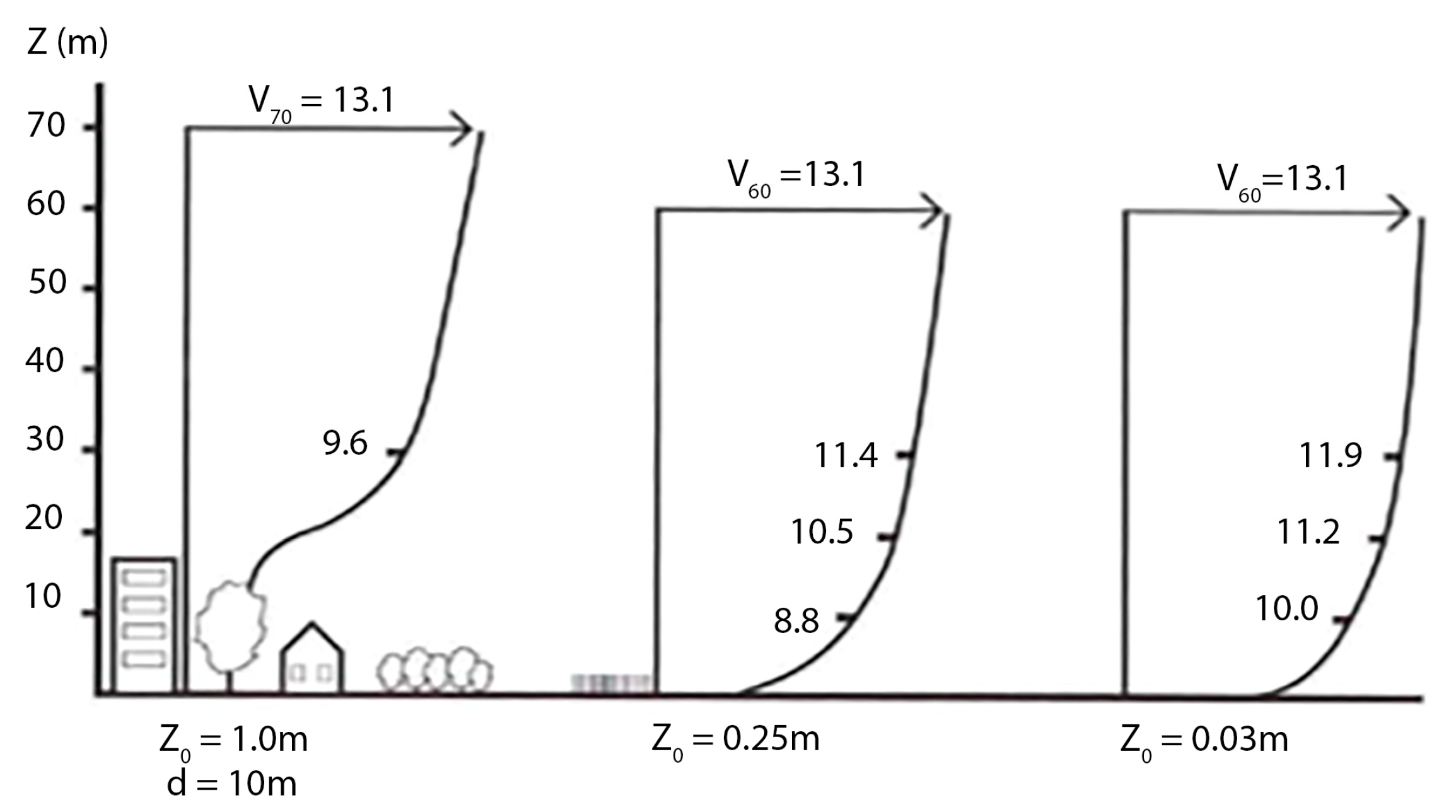
2.2. Microscale Wind Conditions

Terrain roughness, different elements forming the built environment, and geographic features are the factors playing an important role in formulating the microscale wind conditions. The wind flow around buildings is affected greatly by terrain roughness [21,25]. The main types of terrains corresponding to three aerodynamic roughness parameters are (z₀) as follows: city centre terrain (z₀ > 0.7), suburban terrain (z₀ = 0.25–0.3), and open field terrain (z₀ = 0.01–0.03). Based on terrain roughness, the atmospheric boundary layer (ABL) profile, which has the shape of a power law curve, is displaced at a distance d from the ground. In open fields, accessible wind can be reached easily while in cities and areas of urban characteristics, the accessible wind is located at higher altitudes and, in many cases, does not reach the same wind speed as in open fields (Figure 2) [6].

As a first step, macroscale wind conditions need to be assessed, and if the conditions are suitable for urban wind power generation, a more detailed full assessment of the wind resources at the proposed location should be carried out. This assessment will help in deciding the feasibility of installing a wind turbine at the proposed urban location. For large-scale wind power generation, wind farm locations are chosen very carefully to reach the maximum wind resources, while in the case of small-scale wind power generation within the built environment, where many variables affect local urban wind flow, a detailed assessment is needed. It should be noted that relying solely on wind turbines for power supply in urban areas, is not a feasible approach. Urban wind turbines should be considered as a complementary source of renewable energy [15,26].

3. Wind Assessment Tools for the Built Environment

It is evident that the most common research tools used to assess urban wind flow are as follows [27,28,29,30]:

• In situ measurements;
• Wind tunnel tests;
• Computational fluid dynamics simulations (CFD).

Choosing between any of the above-mentioned tools for assessing a specific wind flow scenario depends on their pros and cons. Good design decisions about the type of integration of wind turbines in the vicinity of buildings would be reached by proper implementation of these tools to study the local urban wind flow [31,32,33]. The annual mean wind speed is the main factor affecting the energy yield of the wind turbine; the higher the wind, the more power generated by the wind turbine. Accordingly, it is very important to accurately understand how the wind flows within the proposed location as well as predict or identify the wind speed at the proposed installation location. This plays an important role in determining the feasibility of using a wind turbine in an urban setting [34,35].

Although the previously mentioned tools are the most common in studying urban wind flows, it should be noted that Geographic Information System (GIS) applications play an important role as a start point for providing essential data on wind regimes and urban fabric at a specific location [36]. Thus, coupling the capabilities of wind assessment tools with GIS applications provides reliable data on wind flow regimes in specific locations. This approach reflects positively on a better understanding of urban wind flow resulting in making informed decisions on wind turbine integration within the built environment [37].

One of the main factors affecting the accuracy of wind tunnel tests and CFD simulations is the accuracy of modelling the atmospheric boundary layer (ABL) profile as it is evident that GIS mapping provides accurate data in this regard, which gives more confidence in results from CFD simulations and wind tunnel tests [9]. The application of coupling GIS and urban wind assessment tools is not only useful for urban wind energy applications, but it also covers other forms of renewable energy systems and urban thermal comfort investigation [38].

For urban wind turbine installations, GIS applications provide maps resulting from meteorological and morphological data of urban areas with a focus on wind speed assessment since it is the main factor affecting the energy yield of wind turbines. GIS applications coupled with CFD simulations provide estimates of wind speeds and potential zones for wind turbine installations. However, the data should be carefully processed since these are broad-scale estimates, and finer-scale data are still not readily available. This uncertainty is also attributed to the lack of urban data related to vegetation, building heights, temporary structures, and changes in urban morphology. This could be overcome by newly emerging artificial intelligence (AI) technologies capable of making predictions covering missing data [39].

Accordingly, it is envisioned that AI applications will be filling the gap between coupling GIS and urban wind assessment tools. This approach should be supported by verification and validation studies comparing the results of one tool with verified data produced by another tool, leading to more confidence in the produced data [40].

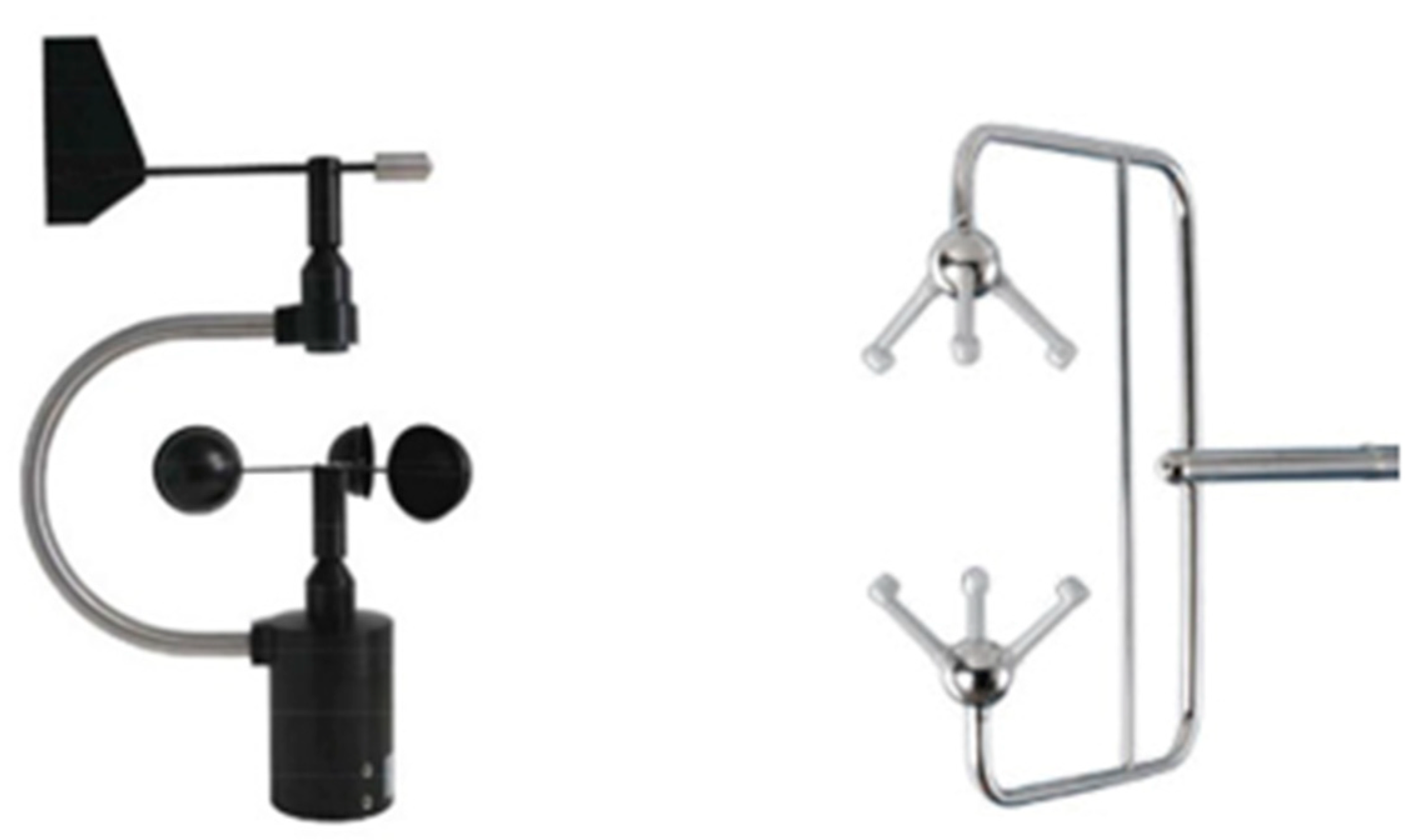
3.1. In Situ Measurements

The device mostly used for full-scale measurements of wind resources is the anemometer. This is the most accurate tool among all tools, especially in the case of roof-mounted wind turbines or integrating wind turbines within completely developed urban areas. The main flow variables affecting the feasibility of the integrated wind turbines are wind velocity, wind direction, and turbulent kinetic energy/turbulence intensity. The anemometer is capable of collecting data about these variables. The most used type of anemometer in urban applications is the cup anemometer. Wind direction is determined by fitting the cup anemometer with a vane, which can correlate the wind velocity with the wind direction (Figure 3) [6,41,42,43,44].

It should be noted that the power available in the wind is determined by air density, which is affected by other variables, such as humidity, temperature, and barometric pressure [45]. Other important data include wind power density at various heights and wind shear coefficient, which could be collected by adding a microwave radiometer and a Doppler lidar [46]. Turbulent kinetic energy, which is a main feature of wind flow in urban areas, is another very important factor, which the cub anemometer cannot measure. A good device that is able to capture wind speed as well as turbulence is the sonic anemometer. Moreover, they are capable of capturing wind direction and recording the vertical wind component. Since they do not have any moving parts, they require less maintenance. The downsides though are the requirements for large data storage capacity and relatively high cost compared with other in situ measurement devices [47].

When installing urban wind power generation devices, the data collected should be very accurate and specific to the location where the wind turbine will be installed. Thus, the measurement tool should be mounted in the exact location where the wind turbine is expected to be installed. While doing this, the prevailing wind direction should be studied carefully and areas of expected high levels of turbulence should be avoided as well as nearby obstacles [34,35]. The collected data should cover a period of at least one year with 10 min intervals between the readings. After that, the collected data are normalised against the data collected over a period of 30 years. It could be argued that the long data collection period is one of the downsides of this tool. In addition to the lengthy process, it is also costly due to the involvement of manpower to carry out maintenance and monitoring of the devices [6,48].

Taking in situ measurements is not an error-free process [49]; errors in this tool could reach 20%, especially in urban areas at the pedestrian level [50]. These errors stem from the over-acceleration of the cup anemometer, which is more responsive to an increase in wind speed than to a decrease in the wind speed of the same value. Thus, the recorded data are expected to be higher than the actual wind speed. The opposite occurs with cup anemometers fitted with a vane since the device does not align immediately with the changing wind direction. These devices miss recording some of the dynamic features of urban wind due to the slow response time of the device to any change in the wind direction [51,52,53].

Erecting the mast to mount the anemometer requires planning permission for a very long period, and the mast itself is an extra cost. These are expensive factors added to the already deemed expensive tool for in situ measurements. The cost should be investigated in the context of the size and energy yield of the proposed wind turbine as this could discourage developers from using in situ measurements as the tool becomes no longer feasible for assessing wind flow at the proposed location. Accordingly, other wind assessment tools could be considered, such as wind tunnel tests and computational fluid dynamics (CFD) simulations. Both have proven to be relatively inexpensive and produce reliable data about urban wind flow if used according to the validated best practice guidelines [45,54].

Of all the advantages of in situ measurements, it is the fact that they produce accurate data at higher levels above the pedestrian street level and they overcome scale mismatch due to Reynolds number (Reynolds number (R_e) is a dimensionless number that gives a measure of the ratio of inertial forces to viscous forces and, consequently, quantifies the relative importance of these two types of forces for given flow conditions. R_e = ρvl/μ Where ρ is the density of the fluid, v is the velocity of the fluid, l is a characteristic linear dimension and μ is the dynamic viscosity), wind shear, and turbulence intensities, or from blockage effects. As for the disadvantages, the cost and the time it takes are the obvious ones. The data are also embedded with errors due to the difficulty of controlling the approach flow conditions. Although in situ measurements are used for the calibration of wind tunnels, it is worth mentioning that the full-scale measurement errors might be, in some cases, larger than the errors in wind tunnel test results. It has been recorded that errors could reach up to 15% in full-scale measurements [55,56,57].

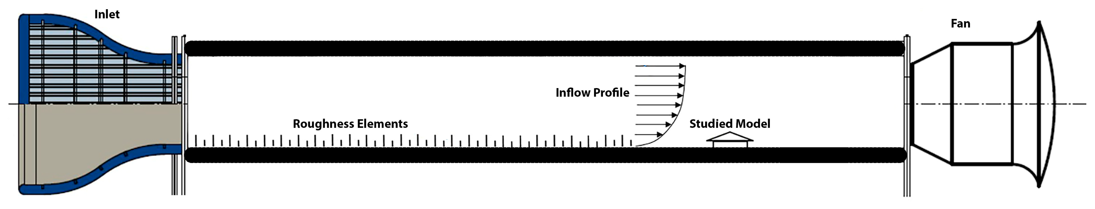
3.2. Wind Tunnel Tests

A wind tunnel test is a good substitute for full-scale on-site measurements since there is more control over the test environment contrary to the unpredictable conditions on in situ measurements. In a wind tunnel test, wind pressure coefficients along buildings’ facades could be calculated with a high level of accuracy, even in highly dense modelled urban areas [57]. Wind tunnel tests have many applications, some of which are calculating wind loads on buildings and investigating pollutant dispersion in urban street canyons, wind comfort at the pedestrian street level, and wind turbine integration in urban areas. Moreover, wind turbine test results could be used for validating data produced by other wind assessment tools [21,58,59,60,61,62,63]. It could be argued that using wind tunnel tests at the early stages of the design gives more flexibility for investigating design alternatives to reach the optimum design solution [21].

Wind tunnel tests were initially developed for industrial engineering and aeronautic applications, but they are currently widely used for investigating wind flow around and inside buildings with applications ranging from natural ventilation in buildings to wind turbine integration. They are also referred to as scale modelling or physical experiments. Using wind tunnels for testing the wind flow is well established in aerodynamics due to the fact that for a long time, they have been tested, validated, and produced reliable results [60]. When wind tunnels were used for urban wind flow applications, they had to be developed according to the complexity of the urban wind flow, which is different from the flow in aeronautic engineering applications where the flow is considered still. This is due to the turbulent nature of the wind flow in urban areas, which means that wind can flow from a variety of directions. Also, the flow is around bluff bodies causing the flow to separate, which is significantly different from the flow around the aerodynamically designed shapes in aeronautical engineering [64].

The early wind tunnels that were used to test urban settings were inaccurate because the applied wind profile at the inlet was uniform across the cross section of the wind tunnel. This is different from the atmospheric boundary layer (ABL) profile, which sees the wind velocity increase with height. This led to the development of wind tunnels able to mimic the actual ABL profile by taking into consideration the variation in wind velocity with height [65,66]. These wind tunnels are called atmospheric boundary layer wind tunnels (BLWTs) and test results obtained from these BLWTs are relatively accurate. To improve the accuracy of the results of the wind flow around a specific building, all surroundings should also be accurately modelled and included inside the wind tunnel (Figure 4) [67].

The dimensions of the atmospheric BLWT are 15–30 m long (the working section) and 2–5 m wide. Wind speed from 10–50 m/s could be tested in these wind tunnels using air under atmospheric pressure. However, it should be noted that reaching the actual wind speed is unnecessary as long as Reynolds numbers are maintained. Usually, the flow variable values are normalised [67,68,69]. Wind speed is not the only flow variable that needs to be simulated since the investigated flow is in urban areas where the flow is characterised as being mostly turbulent. To simulate conditions similar to those in urban areas, a variety of items, such as vortex generators, fences, and spires, are placed in the test section. This results in simulating the turbulent nature of the urban wind flow [21]. Another important factor for increased accuracy of the results from atmospheric BLWT is the scaling similarity, which includes the following [29]:

• Geometric similarity where the ratios of linear dimensions are equal;
• Dynamic similarity where the ratios of forces are equal;
• Kinematic similarity where particle paths are geometrically similar.

Other requirements needed to ensure the accuracy of the wind tunnel test results include the following:

• Accuracy in modelling the mean wind speed, turbulent kinetic energy, and turbulent dissipation rate vertically across the wind tunnel;
• Modelling the important properties of atmospheric turbulence, in particular the relevant length scale of the longitudinal turbulence component, with the same scale approximately the same scale as that used to model buildings or structures;
• Keeping the effect of the longitudinal pressure gradient across the wind tunnel minimal.

Adhering to the above-mentioned requirements would give confidence in wind tunnel test results comparable with the previously discussed in situ measurements. However, due to the difficulty in achieving these requirements accurately, they are considered among the disadvantages of wind tunnel tests. Another disadvantage is the high expense of using techniques such as laser-Doppler anemometry (LDA), particle image velocimetry (PIV), and laser-induced fluorescence (LIF) due to the nature of the wind tunnel test as a point measurement device [65]. Alternative less expensive techniques include hot-wire or hot-film anemometers, Irwin probes, or sand erosion [66].

Wind tunnel tests fall short when it comes to comparing design alternatives. The process becomes costly and time-consuming since the scaled models will need to be rebuilt and the instruments will need to be fine-tuned requiring professional knowledge of how to operate and fine-tune all the used devices. Also, due to the limitation in the size of the wind tunnel, it is very difficult to simulate some flow variables, such as turbulence. Accordingly, corrections need to be made to overcome the inevitable errors resulting from the lack of accuracy in modelling all flow variables [70].

Since the professionals concerned with the built environment are mostly architects, urban planners, and designers, it should be noted that they lack the needed training for using wind tunnels. Thus, they cannot use the tool with confidence, and subsequently, they lose the advantages of using the wind tunnel at the early stages of the design [61]. Due to the familiarity of those professionals with using computer software, CFD simulation packages might be a viable alternative to wind tunnel tests. But accurate wind tunnel tests still remain a good source for producing accurate and reliable data, which could be used for validating CFD simulation results [71].

The challenge that faces wind tunnel tests remains to be the possibility of reproducing the details of the studied urban elements in the scaled physical model, especially when studying low-rise buildings. To overcome this problem, a relatively larger physical model is needed—a model with a scale of at least 1:50 [72]. Obviously, this might not be achievable due to the limitations in the wind tunnel sizes. This also means that the largest turbulence length scales in the wind tunnel are much smaller than the scaled full-scale equivalents. In such situations, the modeller must decide whether to match the turbulence intensity, the integral length scale, or neither, which would affect the accuracy of the results [73]. CFD simulations overcome this problem since the model is virtually a full-scale model.

3.3. Computational Fluid Dynamics (CFD) Simulations

In computational fluid dynamics, the governing equations of fluid dynamics describing the flow of a Newtonian fluid (A Newtonian fluid is a fluid whose stress at each point is linearly proportional to its strain rate at that point. For a Newtonian fluid, the viscosity, by definition, depends only on temperature and pressure, not on the forces acting upon it. If the viscosity does depend on the forces acting upon it then the fluid is said to be non-Newtonian) are solved, which includes the turbulence effect. Similar to wind tunnel tests, CFD simulation was initially developed for aerospace and aeronautical applications [74,75,76]. Recently, CFD has been widely used in studying wind flow around and inside buildings, and the results have been verified and validated and proven to be of the high level of accuracy [77]. Verification and validation studies are very important for increased confidence in CFD simulation results. Thus, it is a viable alternative to wind tunnel tests [78,79]. One of the main advantages of CFD simulations that makes them suitable for urban wind assessment applications is their ability to produce detailed visualisations and point measurements of different flow variables around and inside the studied urban configurations [58,71].

Initially, CFD urban-related applications were focused on studying wind flow for the purpose of natural ventilation in buildings [80], but recently, the applications have covered a wide range of wind flow scenarios around buildings. Other applications include, but not limited to, microscale atmospheric environment around the human body and air flow around and inside buildings with data covering air temperature, velocity, and flow rate [81,82,83].

When comparing CFD to other tools for urban wind assessment, it is relatively more economical than wind tunnel tests and in situ measurements. They are widely used in studying design alternatives for providing high-rise buildings with natural ventilation and enhancing the building form for wind power generation purposes. A good example is the 30 St Mary Axe building by Fosters and Partners, which was previously known as Swiss Re and informally called the Gherkin, where CFD simulations were used for understanding the wind flow at the pedestrian level of the building for the purpose of reducing the turbulence and providing a more comfortable pedestrian level wind flow. This resulted in the tapering form of the lower part of the building we currently see. The tool was also used to improve the atrium’s natural ventilation across the full height of the building [84,85].

Since the 1970s when CFD emerged, researchers [83,86,87,88,89,90,91,92,93,94] have used, studied, and developed the tools, and agreed on the following points as the advantages of CFD simulations:

• CFD simulations are cost-effective when compared with other wind assessment tools, such as in situ measurements and wind tunnel tests. They are even becoming more economical with the increase in computational power.
• When comparing CFD simulations with other tools, CFD simulations can produce a wealth of quantitative and qualitative data across the study domain and not just point measurements.
• CFD simulations are not restricted by the similarity constraints previously discussed.
• CFD simulations are very effective in investigating design alternatives and studying alterations in designs to reach the optimum design solution. This advantage means that CFD speeds up the design process and the design decisions.
• CFD simulations are considered full-scale simulations, which is a big advantage when studying large urban areas or high-rise buildings. The alternative would be wind tunnel tests, which will be limited by the size of the wind tunnel.
• CFD simulations communicate the results easily in the form of meaningful visualisations, which could be understood by the majority of people.

However, CFD simulations also have their disadvantages, which are well documented in the literature [95,96,97,98,99,100,101,102] and need to be carefully considered to mitigate them and make the most out of the tool. The disadvantages are as follows:

• With low computational power, CFD simulations are not very accurate in simulating urban wind flow in high-density built environments. The turbulent nature of the urban wind flow in high-density built environment requires significant computational power.
• There is a high risk of inexperienced users using the tool without professional knowledge of fluid dynamics, which might result in the wrong interpretation of the produced data. The set of skills needed to confidently use CFD simulations is not common among planners, architects, and designers.
• Commercial CFD codes require a wide range of variables to be set up prior to the simulation, such as boundary conditions, turbulence model, grid type, discretisation schemes, adjustments in the ABL profile, etc. If any of these variables is wrong, it will significantly affect the simulation output. Thus, these variables should be specified carefully.
• Due to the complexity of the variables that need to be specified before the simulation, best practice guidelines should be followed as the first step to ensure reliable results, and then, validation against other wind assessment tools should be carried out. In some cases, the validation data are not available; in this case, the results should be treated carefully and interpreted with caution.

Considering the pros and cons of CFD simulations in comparison to the pros and cons of in situ measurements and wind tunnel tests, it can be argued that if the users of CFD simulations are well trained in fluid dynamics and have proper experience in using the tool, CFD simulations would be the most suitable tool for studying the wind flow within the built environment. The ongoing increase in computational power is another factor supporting this argument as CFD simulations have become more accessible for a wide range of people without the need for sophisticated equipment. Thus, CFD is being adopted by many stakeholders concerned with the design and construction of the built environment with wind in mind [103].

3.4. Relevance of Different Tools for Assessing Urban Wind Flow

In terms of flexibility in comparing alternative design solutions, wind tunnel tests and CFD simulations are more flexible than in situ measurements. However, when comparing CFD simulations with wind tunnel tests, CFD simulations provide a good alternative to wind tunnel tests since they are faster in giving reliable results, cheaper than wind tunnel tests, and very powerful when it comes to quantitative and qualitative visualisation of the produced data. There is a good agreement between the two tools in areas around the buildings, but the discrepancies appear at the ground level. The discrepancies stem from near-wall region treatment by the mesh and roughness specifications. The main reason behind this is that in the near-wall area, the flow variables change significantly; also, this area is characterised by vigorous momentum and other scalar transports. Accordingly, the flow in these areas need to be represented accurately, using the relevant turbulence model to yield accurate results [104,105,106].

Generally, there is an agreement in flow trends between wind tunnel test results and CFD simulation results, which suggests that the wind environment needs to be simulated more accurately using both tools. Any difference in results would have implications in terms of making different design decisions. Accordingly, more work is needed to identify the problems in both CFD turbulence simulation and wind tunnel test point measurements [69]. In a study comparing CFD simulation results and wind tunnel test results, discrepancies ranged from 2 to 30% according to the wind direction. However, the results would still be useful due to the agreement in the flow pattern distribution between the two tools [107].

In terms of the expenses associated with using the three tools, they are all deemed relatively expensive to investigate the urban wind flow. As discussed earlier, in situ measurements will yield the most accurate results at the highest cost over the longest period, which leads to the need for more developments in CFD simulation and wind tunnel tests to rely more on them and avoid the expensive and time-consuming in situ measurements. Considering the reviewed literature, the following

Table 1. Comparison between in situ measurements, wind tunnel tests, and CFD simulations.

	Tools Arranged in Descending Order
High accuracy	In Situ Measurements—Wind Tunnel—CFD
High visualisation	CFD—Wind Tunnel—In Situ Measurements
Preference of usage for existing developments	In Situ Measurements—CFD—Wind Tunnel
Preference of usage for future developments	CFD—Wind Tunnel—In Situ Measurements
Lowest cost	CFD—Wind Tunnel—In Situ Measurements
Less time-consuming	CFD—Wind Tunnel—In Situ Measurements
Availability to users	CFD—Wind Tunnel—In Situ Measurements

summarises the comparison between the three tools in terms of accuracy, visualisation capabilities, preference of usage for existing and future planned developments, cost, the required time for assessment, and availability to users.

As seen in the table, of all the investigated tools for studying the wind flow in urban areas, CFD simulation would be the preferred choice for this type of application. The main reasons are that CFD is a powerful tool when it comes to comparing design alternatives, it can also represent the produced data visually more easily, and it is relatively easy to use. However, the users of CFD commercial codes should be well trained in using the codes and have relevant background knowledge to be able to interpret the data confidently. Moreover, the first step in CFD simulation should be following validated best practice guidelines in specifying the simulation parameters; then, validation studies should be carried out before the actual simulation for the flow problem takes place [108].

4. Potential of CFD Simulations as an Urban Wind Assessment Tool

As confirmed by the developers of commercial CFD codes, CFD codes are user-friendly, and with basic knowledge of IT, they are accessible to a wide range of people. Indeed, this is one of the main advantages of CFD simulation software; however, this also means that the software is accessible to users who might not necessarily have the needed understanding of fluid dynamics or the training to use the codes. It is evident that with the ease of using the CFD applications, more architects, planners, and designers are using them to investigate the thermal performance of buildings and air flow inside and outside buildings although they might not have the necessary training or background to use the tool.

Thus, adequate training in using the codes and understanding of at least the basics of fluid dynamics is needed to obtain meaningful results. To prove the importance of the experience needed to use CFD codes, a study was conducted among a group of mechanical engineering graduates who were presented with a flow problem and were asked to use a CFD code to solve the problem. In their first attempt, none of the participants reached the correct answer [109]. This study demonstrates that the experience of the user with the CFD code plays an important role in the accuracy and reliability of the CFD simulation results [70]. Accordingly, not only a background in fluid mechanics engineering is needed for running accurate CFD simulations, but also experience in CFD simulations is needed.

In the following section, the requirements for successful CFD simulations will be reviewed, leading to the most common recommendations for best practice guidelines for using CFD simulations in studying the wind flow in urban areas for wind turbine integration.

4.1. CFD Simulation of the Urban Wind Flow

When studying urban wind flow, the area of interest extends from the ground level up to 200 m high [110]. The fluid/air properties in this boundary layer are characterised by very low variations. The atmospheric boundary layer, the urban boundary layer, and the urban canopy layer need to be modelled accurately to yield reliable results [111]. The Navier–Stokes equations are the governing equations for continuity, momentum, and energy, which represent the conservation laws of physics, within a turbulent flow, and solving these equations provides a description of the flow. They are named after the 18th-century scientists Claude Navier and George Stokes who independently obtained the equations in the first half of the 19th century [35,68,76]. It should be noted that this review focuses on air flow problems and not heat transfer—thus, the concentration on momentum and continuity equations.

The law of conservation of mass governs the continuity equation ensuring that the change of mass in a control volume is equal to the mass that enters through its faces minus the total mass leaving its faces. Newton’s Second Law of Motion (conservation of momentum) governs the momentum equation. It states that the rate of change of momentum of the fluid particles is equal to the total force due to surface stresses and body forces acting in an aligned direction of a chosen coordinate axis. Navier and Stokes combined these principles and expressed them in a set of partial differential equations. Assuming that the flow is incompressible, and the flow nature is three-dimensional, the 3D form of the equations would be:

Continuity equation:

$${\displaystyle \frac{\partial u}{\partial x}}+{\displaystyle \frac{\partial v}{\partial y}}+{\displaystyle \frac{\partial w}{\partial z}}=0$$

(1)

X-component of the momentum equation:

$$\rho {\displaystyle \frac{Du}{Dt}}=-{\displaystyle \frac{\partial p}{\partial x}}+{\displaystyle \frac{\partial {\tau }_{xx}}{\partial x}}+{\displaystyle \frac{\partial {\tau }_{yx}}{\partial y}}+{\displaystyle \frac{\partial {\tau }_{zx}}{\partial z}}+\rho f_x$$

(2)

Y-component of the momentum equation:

$$\rho {\displaystyle \frac{Dv}{Dt}}=-{\displaystyle \frac{\partial p}{\partial y}}+{\displaystyle \frac{\partial {\tau }_{xy}}{\partial x}}+{\displaystyle \frac{\partial {\tau }_{yy}}{\partial y}}+{\displaystyle \frac{\partial {\tau }_{zy}}{\partial z}}+\rho f_y$$

(3)

Z-component of the momentum equation:

$$\rho {\displaystyle \frac{Dw}{Dt}}=-{\displaystyle \frac{\partial p}{\partial z}}+{\displaystyle \frac{\partial {\tau }_{xz}}{\partial x}}+{\displaystyle \frac{\partial {\tau }_{yz}}{\partial y}}+{\displaystyle \frac{\partial {\tau }_{zz}}{\partial z}}+\rho f_z$$

(4)

where u, v, and w are the x, y, and z velocity components, respectively; p is the pressure; ρ is the fluid density; τ is the shear stress; and f_x, f_y, and f_z are the components of the body force per unit mass acting on the fluid [112,113,114].

Computationally, a mesh, which could be regular or irregular, is needed with node points where the flow variables are calculated. The mesh is the division of the domain into a finite number of points or nodes where the flow variables are calculated at specific intervals representing the passage of time. The flow problem is represented in the form of discrete numerical data, which is known as discretisation. Discretisation is divided into three main parts to solve the flow of the fluid—these are equation discretisation, spatial discretisation, and temporal discretisation [76].

In equation discretisation, the governing equations are translated into numerical analogue solvable by the computer. The equations could then be solved by the finite-difference method (FDM), the finite-element method (FEM), or the finite-volume method (FVM). Of the three, it is FDM that is known for its ease in obtaining higher-order accuracy discretisation and, also, for its simplicity. FDM uses a structured cartesian mesh, so it is more used with simple geometries. For complex geometries, FEM could be used since it implements unstructured mesh. This unstructured mesh comes with an expensive computational cost compared with FDM. FVM has the advantage of implementing unstructured and structured meshes; it is known for its efficiency and can be easily programmed [76]. FVM is the most used due to its simplicity in depicting the conservation laws of mass, momentum, and energy in a finite volume of a fluid [76,102].

The equations could be solved by several methods using CFD. However, the numerical method used is recommended to be second-order accurate [115]. In most cases, second-order discretisation schemes obtain a more accurate solution and are preferred for complex flows such as the urban wind flow [116,117,118,119]. A first-order scheme can be used for initial iterations but is not recommended for the final solution. Higher-order schemes require high computational power but are more accurate and efficient. It has been demonstrated that first-order discretisation schemes give inaccurate results and some journals, such as the Journal of Fluid Engineering, do not publish research using first-order discretisation schemes [120]. However, it should be noted the that the First International Workshop on High-Order CFD Methods concluded that higher accuracy is obtained when using high-order methods with smooth geometries, while it was not the case for non-smooth geometries [121].

To solve the equations, the computer goes through an iterative process of trying to solve the equations until the solution converges. Another alternative is that the iterative process repeats until a predefined residual value is reached. The residual value is 0.001 in most commercial CFD codes. For more accurate results, the residual value is set to the lowest possible value. The 0.001 value is considered a relatively high value for a solution to converge, and a residual value that is at least 4 or 5 orders of the magnitude is recommended [115]. Accordingly, a residual value in the range of 10⁻⁴ to 10⁻⁶ residual value is targeted for the solution to converge.

Spatial discretisation is the second category of discretisation. In spatial discretisation, the computational domain is divided by the mesh into smaller subdomains where the flow could be described by its flow variables at the nodes of the mesh at certain time intervals. The main mesh types are the unstructured and structured meshes. The latter is usually used with simple rectilinear geometries while the unstructured mesh is usually used with complex forms. The reason behind using the unstructured mesh for complex forms is that it is made of tetrahedral units that are capable of forming any shape/volume. Obviously, the unstructured grid needs higher computational power. A subcategory of the structured mesh is the multiblock mesh where the domain is divided into zones having different sizes of structured meshes. This is a good way of reducing the required computational power to solve large flow problems. It also gives relatively good control over the mesh when the geometry is complicated [75].

Time/temporal discretisation is the third discretisation category related to unsteady simulations. Here, the time is divided into discrete time steps in the continuous flow. Thus, when compared with the steady-state analysis, there is an additional variable in the governing equations, which is the time (t). In this category, the partial differential equations are in time. So, at a given time, the unknowns are a function of the variables in the previous time step. In this unsteady state, there is an additional step between the equation and spatial discretisation requiring a longer time to solve the equations compared with the steady-state case [112]. There are also many other simulation parameters that need to be specified by the user to accurately set up the flow problem. Due to a lack of experience, the user might mistakenly specify the conditions for the flow problem, which will yield inaccurate results. Accordingly, these parameters need to be identified and accurately specified at the early stages to eradicate any uncertainties and minimize errors in the simulation results.

4.2. CFD Modelling Parameters

CFD codes are embedded with uncertainties, even for experienced users. For consistent simulation results, there are many computational and physical parameters that need to be accurately specified. Accordingly, the literature extensively covers best practice guidelines and quality control in CFD simulation [116,122,123,124,125,126,127]. The five main categories, which are addressed across the literature on CFD simulation best practice guidelines, are defining the physical model, the geometry of the flow problem, the computational domain dimensions, the computational domain boundary conditions, and the computational mesh.

4.2.1. Defining the Physical Model

Defining the physical model is concerned with the physics of the flow by specifying the most suitable turbulence model for solving the basic equations defining the physics of the flow problem. In theory, approximately solving the Navier–Stokes equations means that the flow problem is solved. This is the definition of the direct numerical simulation (DNS) method where a very fine mesh is constructed to capture all flow features, including large and small eddies with any variations happening at each time step. This method is impractical in solving turbulent flow problems due to the enormous computational power needed to handle the number of cells and time steps. However, if the computational power is available to solve the equations in an acceptable period of time, DNS could be used [128,129].

For the equations to be numerically solved, they need to be simplified by filtering out a variety of scales of the turbulent flow. This filtering process means that the basic equations are averaged, which results in more unknowns in the form of sub-grid stresses or turbulence stresses. A turbulence model is used to solve these additional unknowns. The turbulence models have some simplified assumptions, which help in solving the equations [129]. These turbulence models are either time-averaged or space-averaged models, and they are effective in solving turbulent flows. A lot of turbulence models are available for solving turbulent flow problems. The time-averaged method is the most common method, and its models are referred to as Reynolds-averaged Navier–Stokes (RANS) models. As for the space-averaged models, they directly solve the equations governing the large eddies, while the small eddies are modelled using some assumptions. The large eddy simulation (LES) model is a space-filtered model [123]. LES requires very high computational power since it also needs to resolve the flow fields at each time step. The computational power needed for LES remains less than that for DNS, which ignores solving the small eddies not affecting the flow.

A filter function is used in LES to differentiate between small-scale and large-scale eddies. The length scale used as the filter function is the characteristic filter width of the simulation. Eddies larger in length than that length scale are simulated (directly resolved), while eddies smaller than the length scale are modelled (approximated). The main turbulence properties that are not accurately solved by RANS models, such as the von Karman vortex shedding in the wake of an obstacle, could be accurately simulated using this method. This also applies to the recirculation downstream of the windward edges of the studied building and the transient behaviour of separation. But of course, this accuracy comes at a very high computational cost [93,128]. Due to the high computational cost, it is still impractical to use LES although its main advantage is its accuracy in reproducing the average and fluctuating data. But, if sufficient computational power is accessible, then LES could be used to produce data that could be used as a benchmark for comparing the results of other less complex turbulence models, such as the RANS turbulence models [123,130].

Turbulence models should be chosen with care as they have a significant effect on how the flow problem is solved. Each turbulence model has its own advantages, disadvantages, and suitability for solving certain types of flow problems. As a first step, it should be decided whether the flow is steady or unsteady. Since the focus here is on urban wind applications, the flow within the atmospheric boundary layer is expected to be mostly turbulent, thus, unsteady flow assumptions are expected. This will require averaging over small time steps, which is called unsteady RANS (URANS) [128].

However, it should be noted that URANS will not be able to capture the internal fluctuations induced in the flow. For capturing these fluctuations, LES and detached eddy simulation (DES) are recommended. DES implements both RANS and LES; the RANS model is used to solve the flow in the region near the wall while the LES is used for solving the unsteadiness in the wake region of the flow. When comparing this method with using LES across the whole domain, this method significantly consumes less time than LES. But when comparing DES, RANS, and LES, DES will come in between RANS and LES as RANS will still need less time than DES to solve the flow problem. DES also requires experimental data for accurately specifying the inflow boundary conditions; these data are not readily available in practice, and this is why DES is not widely used in wind engineering problems [124,131,132].

Accordingly, it is expected that for the foreseeable future, it is the RANS models that will continue to be used to solve the turbulent wind flow within the built environment in the near-wall region. As seen in Figure 5, each time-dependent variable can be simplified into a fluctuating complement and average value [114].

As an example, the velocity of a turbulent flow at a specific point in time equals the mean velocity of the flow plus the fluctuating velocity component:

$$U=\overline{U}+u^{\prime }$$

(5)

where $\overline{U}$ is the mean velocity taken over a sufficiently long period of time and u′ is its fluctuating component.

Substituting equation (U = $\overline{U}$ + u′) into Navier–Stokes equations, the RANS equations can be obtained:

$${\displaystyle \frac{\partial U_i}{\partial t}}+U_i{\displaystyle \frac{\partial U_i}{\partial x_j}}=-{\displaystyle \frac{1}{\rho }}{\displaystyle \frac{\partial P}{\partial x_i}}+{\displaystyle \frac{\mu }{\rho }}{\displaystyle \frac{\partial }{\partial x_j}} \left({\displaystyle \frac{\partial U_i}{\partial x_j}}-\rho \overline{{u^{\prime }}_i{u^{\prime }}_j}\right)$$

(6)

where U_i is the mean velocity, $P$ is the mean static pressure and $\rho \overline{{u^{\prime }}_i{u^{\prime }}_j}$ are turbulent, or Reynolds, stresses, which are the stresses contributed by turbulent fluctuations. The existence of the stress terms means there is no longer a closed set of equations, and turbulence model assumptions are needed to estimate the unknowns to solve this closure problem. This time averaging raises questions about the efficiency of RANS in solving turbulent flow problems since its turbulence models basically describe a turbulent flow as a steady flow [93,133].

However, it has been shown in many practical applications that RANS results can be sufficiently accurate [123]. In addition, other superior methods, such as LES, still require higher simulation complexity, which comes with a much larger computational power. Accordingly, RANS models can still be used for representing wind flow inside and around buildings. Of the RANS models, it is the k-ε turbulence model that is mostly used; it is a two-equation model and is the most popular RANS turbulence model.

The most recent literature also shows that the k-ω turbulence models can yield reliable and accurate results. The results show agreement with experimental data for reproducing the atmospheric boundary layer (ABL) profile. The drawback of the k-ω turbulence model is in the estimation of the turbulent kinetic energy (TKE) near the building’s walls. The k-ω with shear stress transport (k-ω SST) overcome the overestimation of the pressure in the stagnation zone in the windward façade of the building [134,135,136,137].

Thus, the k-ω turbulence models also provide a good alternative to the k-ε turbulence models for certain flow problems. For example, in simulating drone flight using CFD simulation, the k-ω turbulence model was more accurate in predicting aerodynamic coefficients and pressure distribution than the k-ε turbulence model [138]. However, it should be noted that for urban wind turbine applications where the main concern is wind velocity, the k-ε turbulence models predict the velocity more accurately than the k-ω turbulence models. In a study comparing different turbulence models to predict the flow around a bluff body, the k-ε turbulence model compared more favourably than the k-ω turbulence model in computing pressure distribution along the cube surface and the mean wind velocity, especially in the leeward direction [139].

The same results were obtained in a study where the realizable k-ε turbulence model gave the closest value quantitatively, while the k-ω turbulence model and the standard k-ε turbulence model over- and underpredicted the re-attachment lengths, respectively [140]. Since there should be a fine balance between the accuracy and the time needed for running the simulations, the investigation recommended the realizable k-ε RANS model for reaching this balance for urban wind flow problems. In that study, a variety of turbulence models were tested and the realizable k-ε yielded consistent results without taking a significant time to solve the flow [78].

4.2.2. Flow Problem Geometry

The built environment is geometrically very complicated, which hinders the ability to include all the details of its geometry in the model since the CFD code will take a very long time to solve the flow problem between its parts [141]. However, the area of interest in the model should be reproduced with as much details as possible to the nearest 1 m of detail. Buildings far away from the area of interest are not necessarily important in terms of their geometry and can be included as blocks [124]. The computational domain dimensions will be determined based on the details and dimensions of the buildings to be investigated. The relationship between the building dimensions and the domain dimensions will be discussed in the next section.

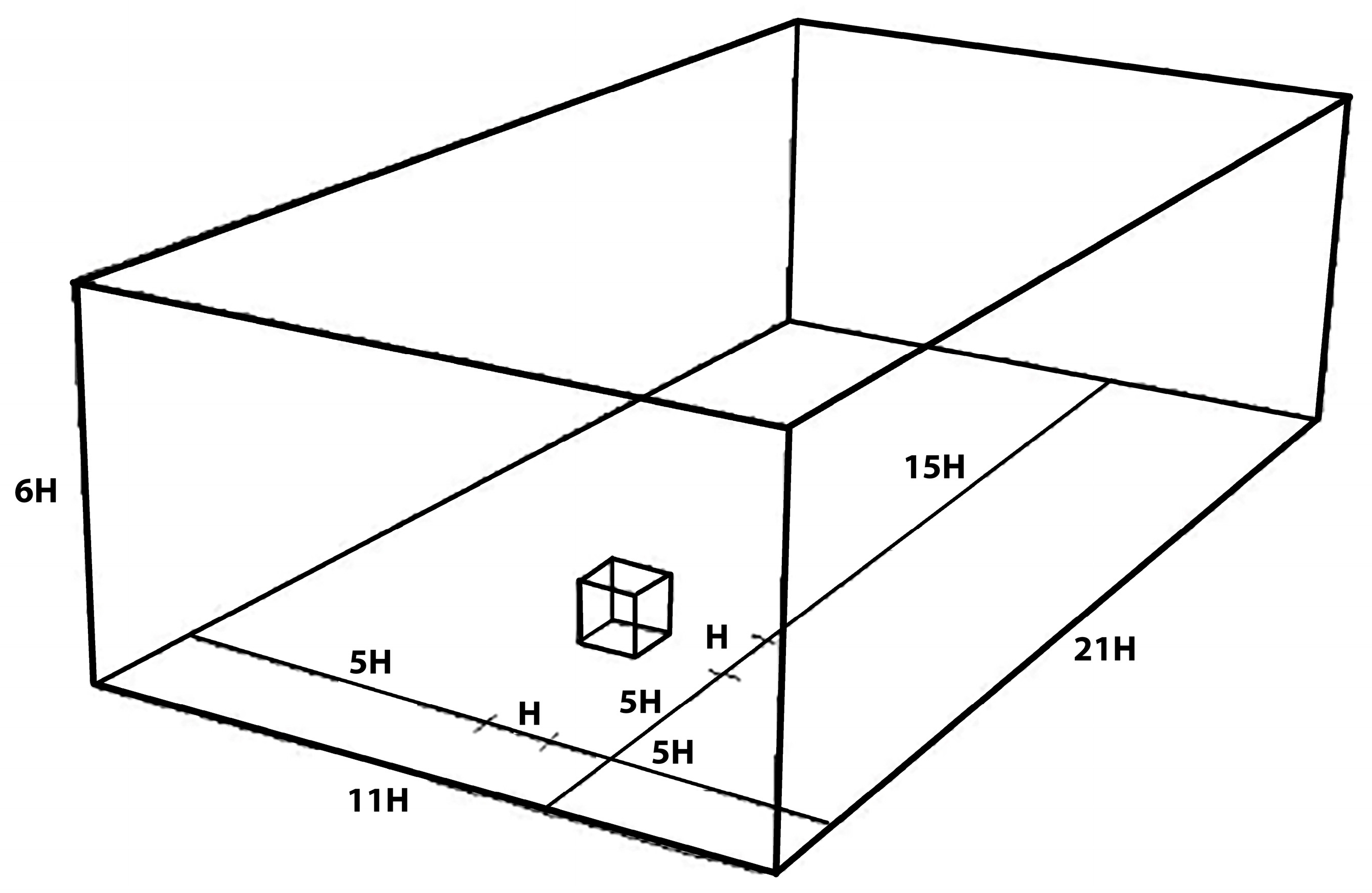
4.2.3. Dimensions of the Computational Domain

The computational domain is a truncation from the real case scenario representing the area of interest. Accordingly, accurately specifying the boundary conditions of the domain plays an important role in the conversion of the solution. Not only specifying the boundary conditions plays an important role in the accuracy of the solution, but also specifying the location or the distance between these boundaries is very important. The distance between the boundaries and the studied area/building should also be specified accurately.

Assuming that the height of the building of interest is H, then the height of the domain should extend five times the height of the building, which makes the total vertical height of the domain six times the height of the highest building (5H) [126,142]. Having this amount of clearance above the highest building prevents any unrealistic flow acceleration above the building [124]. The distance between the two sides of the domain is calculated so that the blockage ratio is a maximum of 3%, where the blockage is defined as the ratio of the projected area of the building in the flow direction to the free cross section of the computational domain. The recommended blockage ratio is 1.5%, which means that a distance of 5H should be allowed between the inlet boundary and the windward facade as well as between the side boundaries and the side facades of the building [126,142]. In the leeward direction of the building, a distance of 15H between the back facade and the outlet of the domain is recommended [70,124,126,142]. Domain dimensions in all directions for a cubic building of specific length H are shown in Figure 6.

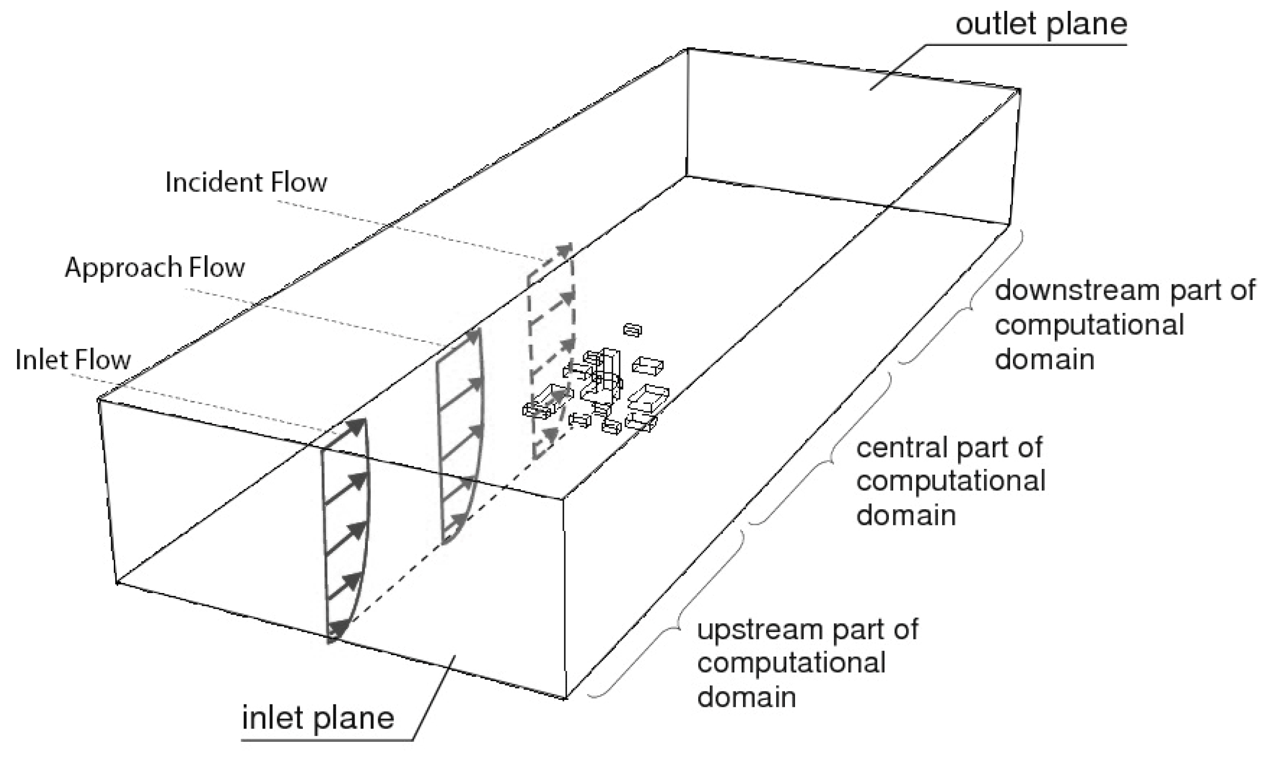
4.2.4. Computational Domain Boundary Conditions

Since the domain is considered a cut through the surrounding of the flow problem, this process means that the artificial boundaries need to have some physical properties minimising the effect of the truncation from the surroundings [112]. Correctly specifying these physical properties, or what is referred to as boundary conditions, is very important for the convergence speed of the solution as well as the accuracy of the simulation. Accordingly, boundary conditions are assigned to the boundaries of the computational domain to simulate the physical quantities in the real flow problem [125]. The main five boundary conditions that need to be assigned in a typical external urban flow problem are the inflow boundary condition, outflow boundary condition, bottom boundary condition, top boundary condition and the side boundary conditions. The top and the side boundary conditions are mostly treated in the same way.

An atmospheric boundary layer (ABL) is assigned to the inflow boundary condition as an inlet. This ABL profile should be consistent for all flow variables across an empty domain until it leaves the domain through the outlet plan. This is what is referred to as the horizontal homogeneity of the ABL profile. The ABL takes the shape of a power exponent or a logarithmic function that describes the changes in the mean wind speed as a function of height due to the variation in the wind speed with height [95,143] (Figure 2). A logarithmic velocity inlet profile is usually used at the inlet. The profile can be obtained from the logarithmic profile corresponding to the upwind terrain through the roughness length (z₀) or from the profiles of the wind tunnel test results; the turbulence quantities at the inlet can be obtained from the assumption of an equilibrium boundary layer, which means that the production and dissipation rates of the turbulent kinetic energy are equal [124].

Using the logarithmic function to compute the velocity profile can be described using the following equation [29]:

$${\displaystyle \frac{V\left(z\right)}{V\left(10\right)}}={\displaystyle \frac{\ln \left(\raisebox{1ex}{$z$}\!\left/ \!\raisebox{-1ex}{$z_0$}\right.\right)}{\ln \left(\raisebox{1ex}{$10$}\!\left/ \!\raisebox{-1ex}{$z_0$}\right.\right)}}$$

(7)

where $V\left(z\right)$ is the wind speed at operating height $z$ (m/s), $z_0$ is the roughness length, and $V\left(10\right)$ is the wind speed (m/s) at a reference height 10 m from the ground. It should be noted that either the power exponent or a logarithmic function can be used to calculate the mean wind velocity or speed at a given height if the mean wind velocity is known at the reference height (z). Parameter $z_0$ represents the roughness length for the type of terrain involved (Figure 2). Another way of obtaining an atmospheric boundary layer (ABL) velocity profile is the empirical formulation known as the power law:

$$V\left(z\right)=V_G{\left({\displaystyle \frac{z}{z_G}}\right)}^{\alpha }$$

(8)

where $V\left(z\right)$ is the wind velocity (m/s) at a height z (m), α is the exponent dependent on terrain conditions, $V_G$ is the wind velocity at the gradient height and $z_G$ is the gradient height. The values in the equations depend on the conditions of the terrain being rural, suburban, or urban (

Table 2. Values of α corresponding to z_G.

Type of Terrain	zG, Gradient Height (m)	α
Open terrain with very few obstacles such as open grass or farmland with few trees, hedgerows, and other barriers; prairie, tundra shores, low islands of inland, lakes, and deserts	300	0.16
Terrain uniformly covered with obstacles 10 to 15 m in height; e.g., residential suburbs, small towns; woodland and shrub, small fields with bushes, trees, and hedges	430	0.28
Terrain with large and irregular objects; e.g., centres of large cities, very broken country with many windbreaks of tall trees, etc.	560	0.40

) [70]. The main advantage of the power law model is its simplicity, and its accuracy is sufficient for most wind engineering applications [21]. On the other hand, the power law models are purely empirical, lacking the support of proven theory, and they are not good for representing the velocity profile close to the ground [70].

As mentioned earlier, the horizontal homogeneity of the ABL profile is an important characteristic of the inlet profile. In other words, the flow variables (velocity, turbulent kinetic energy, and turbulent dissipation rate) across the domain until it reaches the studied building should not change [95,110,144] (Figure 7). The roughness of the bottom wall boundary with the boundary condition of the top boundary helps achieve the horizontal homogeneity of the ABL profile. Thus, tests of the horizontal homogeneity of the ABL profile should be performed in an empty domain before starting to simulate the flow problem. Once the horizontal homogeneity of the ABL profile is achieved, the boundary conditions used in achieving the horizontal homogeneity of the ABL profile could be used in the actual flow problem.

A no-slip wall boundary condition is assigned to the bottom boundary. The flow is greatly affected by this boundary condition since the velocity at the wall surface reaches zero with the maximum value of shear stress. The wall roughness also affects the accuracy of the solution to a great extent—sand-roughened surfaces are implemented by most commercial CFD codes with a corresponding roughness height (k_s) for the roughness of the wall [124]. If that is the case, the following requirements should be satisfied simultaneously [110]:

• High mesh resolution in the vertical direction close to the bottom of the computational domain;
• Maintaining the horizontal homogeneity of the ABL profile upstream and downstream of the computational domain;
• The distance between the centre of the first cell away from the bottom boundary (z_p) and the bottom wall boundary to be greater than the roughness height (z_p > k_s);
• Roughness height equal to thirty times the roughness length (z₀) (k_s = 30 z₀).

Different terrains have different roughness lengths.

Table 3. Roughness parameters for differ terrain categories [145].

Category	z0 (m)	Remark
0	0.003	Corresponding to large expanses of water, mudflats, snow-covered farmland, and large flat areas of tarmac
1	0.01	Corresponding to flat grassland, parkland, or bare soil, without hedges, and with very few isolated obstructions
2	0.03	Meteorological standard, basic terrain roughness corresponding to typical UK farmland, nearly flat or gently undulating countryside, fields with crops, fences or low boundary hedges and few trees
3	0.1	Corresponding to farmland with frequent boundary hedges, occasional small farm structures, houses, or trees
4	0.3	Corresponding to dense woodland, with domestic housing typically between 10% and 20% of plan-area density
5	0.8	Corresponding to city centres, comprising mostly four-storey buildings, or higher, typically between 30% and 50% plan-area density

shows the values of z₀ for six recognizable terrain types in the UK for the design of wind load on buildings and structures. Although it is common sense to have z_p > k_s because it is not physically meaningful to have mesh cells with centre points within the physical roughness height, this would lead to a coarse mesh [110]. Thus, it is recommended to alleviate the requirement z_p > k_s.

To ensure the homogeneity of the inflow profile through the side and top boundary conditions, constant shear stress is applied to the sides corresponding to the inflow profile. A free slip condition at a rigid lid is sometimes used. To achieve the best results, the top and side boundary conditions are specified as symmetry boundary conditions. This means that the flow at the sides and the top of the domain will be parallel and the normal velocity component to the boundary and other flow variables, will disappear, which could be different from the inflow boundary profile [115]. The fluid will mostly leave the computational domain from the boundary behind the studied building/area. This boundary is specified as a constant static pressure or an outflow. Specifying an outflow boundary condition means that all flow variable derivatives are forced to disappear as in a fully developed flow. However, this could result in the flow coming back inside the domain and probably resulting in the solution not reaching convergence. To avoid this and minimise its effect, the boundary is placed far away from the studied building [146].

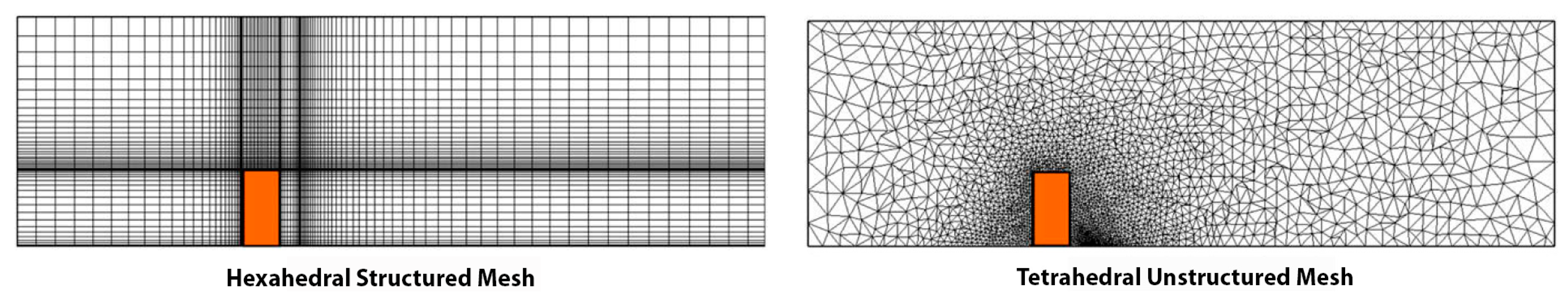
4.2.5. The Computational Mesh

One of the main factors affecting the quality of the CFD simulation is the computational mesh. Thus, care should be taken to construct the mesh and specify its type to be suitable for the flow problem [125,147]. It is agreed that in industrial applications using CFD simulations, most of the time is spent on creating the mesh and adjusting it if needed. This is because a good mesh provides a good balance between the needed computational power and the accuracy of simulation [148]. Due to its important effect on the solution, it is agreed that different mesh sizes and configurations should be used until it is noticed that the solution does not change significantly, and solution is independent of the mesh size [149,150,151,152,153].

The mesh could be refined until the solution does not change. However, this is very time-consuming, which makes the recommendation by Franke et al. (2011) [124] to limit the tested meshes to three levels of refined meshes a viable practice, widely adopted in CFD simulations [154]. The rule of thumb is that the ratio of cells for two consecutive grids should be at least 3.4; sometimes, this is not possible due to computational limitations. If that is the case, it is recommended to refine the mesh in the areas of interest. When studying the wind flow around bluff bodies, the areas where the flow is expected to be more complex are upwind and in the leeward direction of the body and these should be the areas of grid refinements to capture the complicated nature of the flow [70].

Mesh refinement is very problem-dependant, and it is not easy to be specific about the recommendations on mesh resolution [155]. But the general recommendation of the mesh is that the mesh should not deform the geometry of the studied object; ideally, mesh cells should be aligned in an equidistant order, especially in areas of high gradients. It should be noted that sometimes, compression and stretching are permissible as long as the ratio between two consecutive cells does not exceed 1.3 [124].

A good-quality mesh would have the angle between the normal vector of a cell surface and the line connecting the midpoints of the parallel neighbouring cells [156]. Figure 8 shows the shapes of the two types of cells that are either hexahedral or tetrahedral cells. In the structured mesh, hexahedral cells are used, while in the unstructured meshes, tetrahedral cells are mostly used. Hexahedral cells are preferred to tetrahedral cells [157].

In terms of needed computational power, structured meshes are more advantageous over unstructured meshes as the equations are solved faster in structured meshes due to the simplicity of the connectivity between the cells [70]. The main disadvantage of structured meshes is that although they are limited in representing complex shapes and forms, they are good in representing rectilinear simple shapes. However, this problem could be overcome by refining the mesh in the vicinity of complex shapes and geometries. Unstructured meshes, on the other side, are capable of fitting any geometrical form or shape since they are made of tetrahedral units. But this comes with high computational cost due to the complexity of solving the algebraic equations, which is no longer regular as in the structured mesh. Accordingly, more time will be needed for the calculations to take place when using an unstructured mesh.

5. Conclusions

This review discussed the most commonly used urban wind assessment tools, which are in situ measurements, wind tunnel tests, and CFD simulations. The tools were critically investigated to assess their pros and cons. Observations were recorded, and it could be argued that for studying the urban wind flow for the purpose of integrating wind turbines within the built environment, CFD simulation is the most relevant tool. This is mainly due to the iterative nature of the design process and changes that will be made along the way of deciding about the type of wind turbine integration within the built environment as well as the optimum mounting/integration location.

Wind turbine integration within the built environment could use existing buildings or new developments. In existing buildings, all factors affecting the wind flow in the proposed mounting location should be included in the model, and the CFD simulation has high potential in identifying the optimum mounting location in terms of a high mean wind speed and low levels of turbulence. In the case of new developments, alternative design solutions should be investigated, and the CFD simulation tool should be implemented to compare alternative solutions and types of integration. Some of the factors that should be investigated include, but are not limited to, the surrounding urban configuration, site vegetation, and building heights as they will affect the local air flow at the proposed installation site.

CFD simulation as a tool for assessing urban wind flow for urban wind turbine integration was discussed further to identify the requirements for using the tool to yield accurate and consistent results. It can be concluded that available computational power plays a very important role in deciding about a variety of factors affecting the CFD simulation. In addition, the availability of experimental data obtained in wind tunnel tests and in situ measurements is important for validating the CFD simulation results. When comparing RANS, LES, DNS, URANS, and DES models, RANS models are the most commonly used for studying the urban wind flow. However, LES, DNS, URANS, and DES models could yield more accurate results but require higher computational power. Due to the wide usage of RANS models in studying the urban wind flow, there is a wide range of best practice guidelines available in the literature, which are summarised in

Table 4. Best practice guidelines requirements for a reliable CFD simulation.

Solution Method	Second-order schemes or above are recommended for solving algebraic equations.
Residuals	In the range of 10−4 to 10−6.
Mesh	Multiblock structured mesh. Carrying out a sensitivity analysis with three levels of refinements where the ratio of cells for two consecutive grids should be at least 3.4. Mesh cells to be equidistant while refining the mesh in areas of complex flow phenomena. If cells are stretched, a ratio not exceeding 1.3 between two consecutive cells should be maintained.
Turbulence model	Realizable k-ε turbulence model.
Accuracy of studied buildings	Details of dimension equal to or more than 1 m to be included.
Domain dimensions	If H is the building height, the lateral dimension = 2H + building width. Flow direction dimension = 20H + building dimension in the flow direction. Vertical direction = 6H. A blockage ratio below 3% must be maintained.
Boundary conditions	Inflow: horizontally homogenous log law atmospheric boundary layer (ABL) velocity profile. Bottom: a no-slip wall with standard wall functions. Top and side: symmetry. Outflow: pressure outlet.

.

In addition to implementing the above-mentioned requirements as a good start point in the CFD simulation, validation studies using other wind assessment tools are mandatory to eradicate any uncertainties or errors in the CFD simulation. The validation could be carried out by using the recommended parameters for studying the wind flow around a 3D cube mounted in a turbulent channel flow. Data sets from wind tunnel test results as well as in situ instruments for this flow problem are well documented in the literature [73,93,130,158,159,160,161,162,163].

References

1. Ge, J.; Shen, C.; Zhao, K.; Lv, G. Energy production features of rooftop hybrid photovoltaic–wind system and matching analysis with building energy use. Energy Convers. Manag. 2022, 258, 115485. [Google Scholar] [CrossRef]
2. Pellegrini, M.; Guzzini, A.; Saccani, C. Experimental measurements of the performance of a micro-wind turbine located in an urban area. Energy Rep. 2021, 7, 3922–3934. [Google Scholar] [CrossRef]
3. Aravindhan, N.; Natarajan, M.P.; Ponnuvel, S.; Devan, P.K. Recent developments and issues of small-scale wind turbines in urban residential buildings-A review. Energy Environ. 2023, 34, 1142–1169. [Google Scholar] [CrossRef]
4. ArabGolarcheh, A.; Anbarsooz, M.; Benini, E. An actuator line method for performance prediction of HAWTs at urban flow conditions: A case study of rooftop wind turbines. Energy 2024, 292, 130268. [Google Scholar] [CrossRef]
5. Zhang, S.; Du, B.; Ge, M.; Zuo, Y. Study on the operation of small rooftop wind turbines and its effect on the wind environment in blocks. Renew. Energy 2022, 183, 708–718. [Google Scholar] [CrossRef]
6. Stankovic, S.; Campbell, N.; Harries, A. Urban Wind Energy; Routledge: London, UK, 2015. [Google Scholar]
7. Emejeamara, F.C.; Tomlin, A.S. A method for estimating the potential power available to building mounted wind turbines within turbulent urban air flows. Renew. Energy 2020, 153, 787–800. [Google Scholar] [CrossRef]
8. Tong, W. Wind Power Generation and Wind Turbine Design; WIT Press: Southampton, UK, 2010. [Google Scholar]
9. Kwok, K.; Hu, G. Wind energy system for buildings in an urban environment. J. Wind Eng. Ind. Aerodyn. 2023, 234, 105349. [Google Scholar] [CrossRef]
10. Gao, Y.; Yao, R.; Li, B.; Turkbeyler, E.; Luo, Q.; Short, A. Field studies on the effect of built forms on urban wind environments. Renew. Energy 2012, 46, 148–154. [Google Scholar] [CrossRef]
11. Walker, S.L. Building mounted wind turbines and their suitability for the urban scale—A review of methods of estimating urban wind resource. Energy Build. 2011, 43, 1852–1862. [Google Scholar] [CrossRef]
12. Moscoloni, C.; Zarra, F.; Novo, R.; Giglio, E.; Vargiu, A.; Mutani, G.; Bracco, G.; Mattiazzo, G. Wind turbines and rooftop photovoltaic technical potential assessment: Application to sicilian minor islands. Energies 2022, 15, 5548. [Google Scholar] [CrossRef]
13. Javaid, A.; Sajid, M.; Uddin, E.; Waqas, A.; Ayaz, Y. Sustainable urban energy solutions: Forecasting energy production for hybrid solar-wind systems. Energy Convers. Manag. 2024, 302, 118120. [Google Scholar] [CrossRef]
14. Gür, M.; Karadag, I. Machine Learning for Pedestrian-Level Wind Comfort Analysis. Buildings 2024, 14, 1845. [Google Scholar] [CrossRef]
15. Simões, T.; Estanqueiro, A. A new methodology for urban wind resource assessment. Renew. Energy 2016, 89, 598–605. [Google Scholar] [CrossRef]
16. Lu, L.; Sun, K. Wind power evaluation and utilization over a reference high-rise building in urban area. Energy Build. 2014, 68, 339–350. [Google Scholar] [CrossRef]
17. Zhang, R.; Xu, X.; Liu, K.; Kong, L.; Wang, W.; Wortmann, T. Airflow modelling for building design: A designers’ review. Renew. Sustain. Energy Rev. 2024, 197, 114380. [Google Scholar] [CrossRef]
18. Shou, S.; Li, S.; Shou, Y.; Yao, X. An Introduction to Mesoscale Meteorology; Springer: Singapore, 2023. [Google Scholar]
19. Dannecker, R.K. Wind Energy in the Built Environment: An Experimental and Numerical Investigation of a Building Integrated Ducted Wind Turbine Module. Ph.D. Thesis, University of Strathclyde, Glasgow, UK, 2001. [Google Scholar]
20. Meyer, S. A new perspective on surface weather maps. Sci. Act. 2006, 42, 3–9. [Google Scholar] [CrossRef]
21. Cermak, J.E. Wind Tunnel Studies of Buildings and Structures; American Society of Civil Engineers: Reston, VA, USA, 1999. [Google Scholar]
22. Ackermann, T.; Söder, L. An overview of wind energy-status 2002. Renew. Sustain. Energy Rev. 2002, 6, 67–127. [Google Scholar] [CrossRef]
23. Ricciardelli, F.; Polimeno, S. Some characteristics of the wind flow in the lower Urban Boundary Layer. J. Wind Eng. Ind. Aerodyn. 2006, 94, 815–832. [Google Scholar] [CrossRef]
24. Tadie Fogaing, M.B.; Gordon, H.; Lange, C.F.; Wood, D.H.; Fleck, B.A. A review of wind energy resource assessment in the urban environment. In Advances in Sustainable Energy; Springer: Cham, Switzerland, 2019; pp. 7–36. [Google Scholar]
25. Jie, P.; Su, M.; Gao, N.; Ye, Y.; Kuang, X.; Chen, J.; Li, P.; Grunewald, J.; Xie, X.; Shi, X. Impact of urban wind environment on urban building energy: A review of mechanisms and modeling. Build. Environ. 2023, 245, 110947. [Google Scholar] [CrossRef]
26. Herbert, G.J.; Iniyan, S.; Amutha, D. A review of technical issues on the development of wind farms. Renew. Sustain. Energy Rev. 2014, 32, 619–641. [Google Scholar] [CrossRef]
27. Chen, Q.Y. Using computational tools to factor wind into architectural environment design. Energy Build. 2004, 36, 1197–1209. [Google Scholar] [CrossRef]
28. Mertens, S. Wind Energy in the Built Environment; Multi Science Publishing Company: Brentwood, UK, 2005. [Google Scholar]
29. Jha, A.R. Wind Turbine Technology; CRC Press: Boca Raton, FL, USA, 2011. [Google Scholar]
30. Gil-García, I.C.; García-Cascales, M.S.; Molina-García, A. Urban wind: An alternative for sustainable cities. Energies 2022, 15, 4759. [Google Scholar] [CrossRef]
31. Bobrova, D. Building-integrated wind turbines in the aspect of architectural shaping. Procedia Eng. 2015, 117, 404–410. [Google Scholar] [CrossRef]
32. Campos-Arriaga, L. Wind Energy in the Built Environment: A Design Analysis Using CFD and Wind Tunnel Modelling Approach. Ph.D. Thesis, University of Nottingham, Nottingham, UK, 2009. [Google Scholar]
33. Li, Q.S.; Shu, Z.R.; Chen, F.B. Performance assessment of tall building-integrated wind turbines for power generation. Appl. Energy 2016, 165, 777–788. [Google Scholar] [CrossRef]
34. Arteaga-López, E.; Ángeles-Camacho, C.; Bañuelos-Ruedas, F. Advanced methodology for feasibility studies on building-mounted wind turbines installation in urban environment: Applying CFD analysis. Energy 2019, 167, 181–188. [Google Scholar] [CrossRef]
35. Anup, K.C.; Whale, J.; Urmee, T. Urban wind conditions and small wind turbines in the built environment: A review. Renew. Energy 2019, 131, 268–283. [Google Scholar]
36. Vallejo, A.; Herrera, I.; Castellanos, J.E.; Pereyra, C.; Garabitos, E. Urban wind potential analysis: Case study of wind turbines integrated into a building using onsite measurements and CFD modelling. In Proceedings of the 36th International Conference on Efficiency, Cost, Optimization, Simulation and Environmental Impact of Energy Systems, Las Palmas de Gran Canaria, Spain, 25–30 June 2023. [Google Scholar]
37. Back, Y.; Kumar, P.; Bach, P.M.; Rauch, W.; Kleidorfer, M. Integrating CFD-GIS modelling to refine urban heat and thermal comfort assessment. Sci. Total Environ. 2023, 858, 159729. [Google Scholar] [CrossRef]
38. Gagliano, A.; Nocera, F.; Patania, F.; Capizzi, A. Assessment of micro-wind turbines performance in the urban environments: An aided methodology through geographical information systems. Int. J. Energy Environ. Eng. 2013, 4, 43. [Google Scholar] [CrossRef]
39. Liu, Y.; Yigitcanlar, T.; Guaralda, M.; Degirmenci, K.; Liu, A. Spatial Modelling of Urban Wind Characteristics: Review of Contributions to Sustainable Urban Development. Buildings 2024, 14, 737. [Google Scholar] [CrossRef]
40. Tominaga, Y.; Wang, L.; Zhai, Z.; Stathopoulos, T. Accuracy of CFD simulations in urban aerodynamics and microclimate: Progress and challenges. Build. Environ. 2023, 243, 110723. [Google Scholar] [CrossRef]
41. Bartko, M.; Molleti, S.; Baskaran, A. In situ measurements of wind pressures on low slope membrane roofs. J. Wind Eng. Ind. Aerodyn. 2016, 153, 78–91. [Google Scholar] [CrossRef]
42. Plate, E.J. Methods of investigating urban wind fields—Physical models. Atmos. Environ. (1994) 1999, 33, 3981–3989. [Google Scholar] [CrossRef]
43. Dubov, D.; Aprahamian, B.; Aprahamian, M. Comparison of wind data measurment results of LIDAR device and calibrated cup anemometers mounted on a met mast. In Proceedings of the 2018 20th International Symposium on Electrical Apparatus and Technologies (SIELA), Bourgas, Bulgaria, 3–6 June 2018; pp. 1–4. [Google Scholar]
44. Karthikeya, B.R.; Negi, P.S.; Srikanth, N. Wind resource assessment for urban renewable energy application in Singapore. Renew Energy 2016, 87, 403–414. [Google Scholar] [CrossRef]
45. Anderson, D.C.; Whale, J.; Livingston, P.O.; Chan, D. Rooftop wind resource assessment using a three-dimension ultrasonic anemometer. In Proceedings of the 7th World Wind Energy Conference, Kingston, ON, Canada, 24–26 June 2008. [Google Scholar]
46. He, J.Y.; Chan, P.W.; Li, Q.S.; Huang, T.; Yim, S.H.L. Assessment of urban wind energy resource in Hong Kong based on multi-instrument observations. Renew. Sustain. Energy Rev. 2024, 191, 114123. [Google Scholar] [CrossRef]
47. Nosov, V.; Lukin, V.; Nosov, E.; Torgaev, A.; Bogushevich, A. Measurement of Atmospheric Turbulence Characteristics by the Ultrasonic Anemometers and the Calibration Processes. Atmosphere 2019, 10, 460. [Google Scholar] [CrossRef]
48. Stathopoulos, T.; Alrawashdeh, H.; Al-Quraan, A.; Blocken, B.; Dilimulati, A.; Paraschivoiu, M.; Pilay, P. Urban wind energy: Some views on potential and challenges. J. Wind Eng. Ind. Aerodyn. 2018, 179, 146–157. [Google Scholar] [CrossRef]
49. Azorin-Molina, C.; Pirooz, A.A.S.; Bedoya-Valestt, S.; Utrabo-Carazo, E.; Andres-Martin, M.; Shen, C.; Minola, L.; Guijarro, J.A.; Aguilar, E.; Brunet, M.; et al. Biases in wind speed measurements due to anemometer changes. Atmos. Res. 2023, 289, 106771. [Google Scholar] [CrossRef]
50. Willemsen, E.; Wisse, J.A. Accuracy of assessment of wind speed in the built environment. J. Wind Eng. Ind. Aerodyn. 2002, 90, 1183–1190. [Google Scholar] [CrossRef]
51. Kaganov, E.I.; Iaglom, A.M. Errors in wind-speed measurements by rotation anemometers. Bound.-Layer Meteorol. 1976, 10, 15–34. [Google Scholar] [CrossRef]
52. Kennedy, J.J. A review of uncertainty in in situ measurements and data sets of sea surface temperature. Rev. Geophys. 2014, 52, 1–32. [Google Scholar] [CrossRef]
53. Morris, V.R.; Barnard, J.C.; Wendell, L.L.; Tomich, S.D. Comparison of anemometers for turbulence characterization. In Proceedings of the Windpower ‘92, Seattle, WA, USA, 19–23 October 1992. [Google Scholar]
54. Reja, R.K.; Amin, R.; Tasneem, Z.; Ali, M.F.; Islam, M.R.; Saha, D.K.; Badal, F.R.; Ahamed, M.H.; Moyeen, S.I.; Das, S.K. A review of the evaluation of urban wind resources: Challenges and perspectives. Energy Build. 2022, 257, 111781. [Google Scholar] [CrossRef]
55. Easom, G. Improved Turbulence Models for Computational Wind Engineering. Ph.D. Thesis, University of Nottingham, Nottingham, UK, 2000. [Google Scholar]
56. Yang, T. CFD and Field Testing of a Naturally Ventilated Full-Scale Building. Ph.D. Thesis, University of Nottingham, Nottingham, UK, 2004. [Google Scholar]
57. Cheng, X.; Zhao, L.; Ge, Y.; Dong, J.; Peng, Y. Full-Scale/Model Test Comparisons to Validate the Traditional Atmospheric Boundary Layer Wind Tunnel Tests: Literature Review and Personal Perspectives. Appl. Sci. 2024, 14, 782. [Google Scholar] [CrossRef]
58. Blocken, B.; Stathopoulos, T.; van Beeck, J.P.A.J. Pedestrian-level wind conditions around buildings: Review of wind-tunnel and CFD techniques and their accuracy for wind comfort assessment. Build. Environ. 2016, 100, 50–81. [Google Scholar] [CrossRef]
59. Bottasso, C.L.; Campagnolo, F.; Petrović, V. Wind tunnel testing of scaled wind turbine models: Beyond aerodynamics. J. Wind Eng. Ind. Aerodyn. 2014, 127, 11–28. [Google Scholar] [CrossRef]
60. Chanetz, B. A century of wind tunnels since Eiffel. C. R. Mécanique 2017, 345, 581–594. [Google Scholar] [CrossRef]
61. Irwin, P.; Denoon, R.; Scott, D. Wind Tunnel Testing of High-Rise Buildings; Routledge: London, UK, 2013. [Google Scholar]
62. Janhäll, S. Review on urban vegetation and particle air pollution—Deposition and dispersion. Atmos. Environ. 2015, 105, 130–137. [Google Scholar] [CrossRef]
63. Longo, S.G. Applications in Wind Tunnel Technology. In Principles and Applications of Dimensional Analysis and Similarity; Springer: Cham, Switzerland, 2022. [Google Scholar]
64. Lawson, T. Building Aerodynamics; Imperial College Press: London, UK, 2001. [Google Scholar]
65. Blocken, B.; Carmeliet, J. Pedestrian Wind Environment around Buildings: Literature Review and Practical Examples. J. Therm. Envel. Build. Sci. 2004, 28, 107–159. [Google Scholar] [CrossRef]
66. Stathopoulos, T.; Blocken, B. Pedestrian wind environment around tall buildings. In Advanced Environmental Wind Engineering; Springer: Tokyo, Japan, 2016; pp. 101–127. [Google Scholar]
67. Janke, D.; Yi, Q.; Thormann, L.; Hempel, S.; Amon, B.; Nosek, Š.; van Overbeke, P.; Amon, T. Direct Measurements of the Volume Flow Rate and Emissions in a Large Naturally Ventilated Building. Sensors 2020, 20, 6223. [Google Scholar] [CrossRef]
68. Aly, A.M. Atmospheric boundary-layer simulation for the built environment: Past, present and future. Build. Environ. 2014, 75, 206–221. [Google Scholar] [CrossRef]
69. Jones, P.J.; Alexander, D.; Burnett, J. Pedestrian Wind Environment Around High-Rise Residential Buildings in Hong Kong. Indoor Built Environ. 2004, 13, 259–269. [Google Scholar] [CrossRef]
70. Hu, C.H. Proposed Guidelines of Using CFD And the Validity of the CFD Models in the Numerical Simulations of Wind Environments around Buildings. Ph.D. Thesis, Heriot-Watt University, Edinburgh, UK, 2003. [Google Scholar]
71. Reiter, S. Assessing Wind Comfort in Urban Planning. Environ. Plan. B Plan. Des. 2010, 37, 857–873. [Google Scholar] [CrossRef]
72. Tieleman, H.W. Wind tunnel simulation of wind loading on low-rise structures: A review. J. Wind Eng. Ind. Aerodyn. 2003, 91, 1627–1649. [Google Scholar] [CrossRef]
73. Richards, P.J.; Hoxey, R.P.; Connell, B.D.; Lander, D.P. Wind-tunnel modelling of the Silsoe Cube. J. Wind Eng. Ind. Aerodyn. 2007, 95, 1384–1399. [Google Scholar] [CrossRef]
74. Çengel, Y.A.; Cimbala, J.M. Fluid Mechanics; McGraw-Hill Education: New York, NY, USA, 2018. [Google Scholar]
75. Wen, T.; Lu, L.; He, W.; Min, Y. Fundamentals and applications of CFD technology on analyzing falling film heat and mass exchangers: A comprehensive review. Appl. Energy 2020, 261, 114473. [Google Scholar] [CrossRef]
76. Zawawi, M.H.; Saleha, A.; Salwa, A.; Hassan, N.H.; Zahari, N.M.; Ramli, M.Z.; Muda, Z.C. A review: Fundamentals of computational fluid dynamics (CFD). AIP Conf. Proc. 2018, 2030, 020252. [Google Scholar]
77. Mirzaei, P.A. CFD modeling of micro and urban climates: Problems to be solved in the new decade. Sustain. Cities Soc. 2021, 69, 102839. [Google Scholar] [CrossRef]
78. Blocken, B.; Stathopoulos, T.; Carmeliet, J.; Hensen, J.L.M. Application of computational fluid dynamics in building performance simulation for the outdoor environment: An overview. J. Build. Perform. Simul. 2011, 4, 157–184. [Google Scholar] [CrossRef]
79. Kim, D. The Application of CFD to Building Analysis and Design: A Combined Approach of an Immersive Case Study and Wind Tunnel Testing. Ph.D. Thesis, Virginia Tech, Blacksburg, VA, USA, 2013. [Google Scholar]
80. Jones, P.J.; Whittle, G.E. Computational fluid dynamics for building air flow prediction—Current status and capabilities. Build. Environ. 1992, 27, 321–338. [Google Scholar] [CrossRef]
81. Runchal, A. 50 Years of CFD in Engineering Sciences; Springer: Singapore, 2020. [Google Scholar]
82. Zhai, Z. Application of Computational Fluid Dynamics in Building Design: Aspects and Trends. Indoor Built Environ. 2006, 15, 305–313. [Google Scholar] [CrossRef]
83. Wijesooriya, K.; Mohotti, D.; Lee, C.; Mendis, P. A technical review of computational fluid dynamics (CFD) applications on wind design of tall buildings and structures: Past, present and future. J. Build. Eng. 2023, 74, 106828. [Google Scholar] [CrossRef]
84. Acred, A. Natural ventilation in multi-storey buildings: A preliminary design approach. Ph.D. Thesis, Imperial College London, UK, 2014. [Google Scholar]
85. Kamal, M.A.; Ahmed, E. Analyzing Energy Efficient Design Strategies in High-rise Buildings with Reference to HVAC System. Archit. Eng. Sci. 2023, 4, 183. [Google Scholar] [CrossRef]
86. Ai, Z.T.; Mak, C.M. CFD simulation of flow in a long street canyon under a perpendicular wind direction: Evaluation of three computational settings. Build. Environ. 2017, 114, 293–306. [Google Scholar] [CrossRef]
87. Bernardini, E.; Spence, S.M.J.; Wei, D.; Kareem, A. Aerodynamic shape optimization of civil structures: A CFD-enabled Kriging-based approach. J. Wind Eng. Ind. Aerodyn. 2015, 144, 154–164. [Google Scholar] [CrossRef]
88. Bustamante, E.; García-Diego, F.; Calvet, S.; Estellés, F.; Beltrán, P.; Hospitaler, A.; Torres, A. Exploring Ventilation Efficiency in Poultry Buildings: The Validation of Computational Fluid Dynamics (CFD) in a Cross-Mechanically Ventilated Broiler Farm. Energies 2013, 6, 2605–2623. [Google Scholar] [CrossRef]
89. Hensen, J.; Bartak, M.; Drkal, F. Modeling and simulation of a double-skin facade system. ASHRAE Trans. 2002, 108, 1251–1259. [Google Scholar]
90. Kaseb, Z.; Hafezi, M.; Tahbaz, M.; Delfani, S. A framework for pedestrian-level wind conditions improvement in urban areas: CFD simulation and optimization. Build. Environ. 2020, 184, 107191. [Google Scholar] [CrossRef]
91. Mistriotis, A.; De Jong, T.; Wagemans, M.J.M.; Bot, G.P.A. Computational Fluid Dynamics (CFD) as a tool for the analysis of ventilation and indoor microclimate in agricultural buildings. Neth. J. Agric. Sci. 1997, 45, 81–96. [Google Scholar] [CrossRef]
92. Tan, G.; Glicksman, L.R. Application of integrating multi-zone model with CFD simulation to natural ventilation prediction. Energy Build. 2005, 37, 1049–1057. [Google Scholar] [CrossRef]
93. Toja-Silva, F.; Kono, T.; Peralta, C.; Lopez-Garcia, O.; Chen, J. A review of computational fluid dynamics (CFD) simulations of the wind flow around buildings for urban wind energy exploitation. J. Wind Eng. Ind. Aerodyn. 2018, 180, 66–87. [Google Scholar] [CrossRef]
94. Tominaga, Y.; Stathopoulos, T. CFD simulations can be adequate for the evaluation of snow effects on structures. Build. Simul 2020, 13, 729–737. [Google Scholar] [CrossRef]
95. Abohela, I.; Aristodemou, E.; Hadawey, A.; Sundararajan, R. Assessing the Horizontal Homogeneity of the Atmospheric Boundary Layer (HHABL) Profile Using Different CFD Software. Atmosphere 2020, 11, 1138. [Google Scholar] [CrossRef]
96. Aflaki, A.; Esfandiari, M.; Mohammadi, S. A Review of Numerical Simulation as a Precedence Method for Prediction and Evaluation of Building Ventilation Performance. Sustainability 2021, 13, 12721. [Google Scholar] [CrossRef]
97. Ai, Z.T.; Mak, C.M. Potential use of reduced-scale models in CFD simulations to save numerical resources: Theoretical analysis and case study of flow around an isolated building. J. Wind Eng. Ind. Aerodyn. 2014, 134, 25–29. [Google Scholar] [CrossRef]
98. Chong, W.T.; Pan, K.C.; Poh, S.C.; Fazlizan, A.; Oon, C.S.; Badarudin, A.; Nik-Ghazali, N. Performance investigation of a power augmented vertical axis wind turbine for urban high-rise application. Renew. Energy 2013, 51, 388–397. [Google Scholar] [CrossRef]
99. Ramponi, R.; Blocken, B.; de Coo, L.B.; Janssen, W.D. CFD simulation of outdoor ventilation of generic urban configurations with different urban densities and equal and unequal street widths. Build. Environ. 2015, 92, 152–166. [Google Scholar] [CrossRef]
100. Sabatino, S.D.; Buccolieri, R.; Pulvirenti, B.; Britter, R.E. Flow and Pollutant Dispersion in Street Canyons using FLUENT and ADMS-Urban. Environ. Model. Assess. 2008, 13, 369–381. [Google Scholar] [CrossRef]
101. Santiago, J.L.; Borge, R.; Martin, F.; de la Paz, D.; Martilli, A.; Lumbreras, J.; Sanchez, B. Evaluation of a CFD-based approach to estimate pollutant distribution within a real urban canopy by means of passive samplers. Sci. Total Environ. 2017, 576, 46–58. [Google Scholar] [CrossRef] [PubMed]
102. Weerasuriya, A.U.; Hu, Z.Z.; Zhang, X.L.; Tse, K.T.; Li, S.; Chan, P.W. New inflow boundary conditions for modeling twisted wind profiles in CFD simulation for evaluating the pedestrian-level wind field near an isolated building. Build. Environ. 2018, 132, 303–318. [Google Scholar] [CrossRef]
103. Meroney, R.N. Ten questions concerning hybrid computational/physical model simulation of wind flow in the built environment. Build. Environ. 2016, 96, 12–21. [Google Scholar] [CrossRef]
104. Calautit, J.K.; Hughes, B.R. Wind tunnel and CFD study of the natural ventilation performance of a commercial multi-directional wind tower. Build. Environ. 2014, 80, 71–83. [Google Scholar] [CrossRef]
105. Irtaza, H.; Beale, R.G.; Godley, M.H.R.; Jameel, A. Comparison of wind pressure measurements on Silsoe experimental building from full-scale observation, wind-tunnel experiments and various CFD techniques. Int. J. Eng. Sci. Technol. 2018, 5, 28–41. [Google Scholar] [CrossRef]
106. Kosutova, K.; van Hooff, T.; Vanderwel, C.; Blocken, B.; Hensen, J. Cross-ventilation in a generic isolated building equipped with louvers: Wind-tunnel experiments and CFD simulations. Build. Environ. 2019, 154, 263–280. [Google Scholar] [CrossRef]
107. Kim, T.; Kim, K.; Kim, B.S. A wind tunnel experiment and CFD analysis on airflow performance of enclosed-arcade markets in Korea. Build. Environ. 2010, 45, 1329–1338. [Google Scholar] [CrossRef]
108. Hågbo, T.; Giljarhus, K.E.T. Sensitivity of urban morphology and the number of CFD simulated wind directions on pedestrian wind comfort and safety assessments. Build. Environ. 2024, 253, 111310. [Google Scholar] [CrossRef]
109. Chen, Q.; Zhai, Z. The use of Computational Fluid Dynamics tools for indoor environmental design. In Advanced Building Simulation; Routledge: London, UK, 2004; pp. 133–154. [Google Scholar]
110. Blocken, B.; Stathopoulos, T.; Carmeliet, J. CFD simulation of the atmospheric boundary layer: Wall function problems. Atmos. Environ. 2007, 41, 238–252. [Google Scholar] [CrossRef]
111. Potsis, T.; Tominaga, Y.; Stathopoulos, T. Computational wind engineering: 30 years of research progress in building structures and environment. J. Wind Eng. Ind. Aerodyn. 2023, 234, 105346. [Google Scholar] [CrossRef]
112. Blazek, J. Computational Fluid Dynamics; Elsevier/Butterworth-Heinemann: Amsterdam, The Netherlands, 2015. [Google Scholar]
113. Cebeci, T.; Shao, J.P.; Kafyeke, F.; Laurendeau, E. Computational Fluid Dynamics for Engineers: From Panel to Navier-Stokes Methods with Computer Programs; Springer: Berlin/Heidelberg, Germany, 2005. [Google Scholar]
114. Versteeg, H.K.; Malalasekera, W. An Introduction to Computational Fluid Dynamics: The Finite Volume Method; Pearson/Prentice Hall: Upper Saddle River, NJ, USA, 2007. [Google Scholar]
115. Franke, J. Recommendations of the Cost Action C14 on the Use of CFD in Predicting Pedestrian Wind Environment. J. Wind Eng. 2006, 31, 529–532. [Google Scholar] [CrossRef]
116. Sørensen, D.N.; Nielsen, P.V. Quality control of computational fluid dynamics in indoor environments. Indoor Air 2003, 13, 2–17. [Google Scholar] [CrossRef]
117. Deng, X.; Mao, M.; Tu, G.; Zhang, H.; Zhang, Y. High-Order and High Accurate CFD Methods and Their Applications for Complex Grid Problems. Commun. Comput. Phys. 2012, 11, 1081–1102. [Google Scholar] [CrossRef]
118. Lemaire, S.; Vaz, G.; Deij-van Rijswijk, M.; Turnock, S.R. On the accuracy, robustness, and performance of high order interpolation schemes for the overset method on unstructured grids. Int. J. Numer. Methods Fluids 2022, 94, 152–187. [Google Scholar] [CrossRef]
119. Wang, Z.J. High-order methods for the Euler and Navier–Stokes equations on unstructured grids. Prog. Aerosp. Sci. 2007, 43, 1–41. [Google Scholar] [CrossRef]
120. Freitas, C.J. Policy Statement on the Control of Numerical Accuracy. Trans. ASME J. Fluids Eng. 1993, 115, 339–340. [Google Scholar]
121. Wang, Z.J.; Fidkowski, K.; Abgrall, R.; Bassi, F.; Caraeni, D.; Cary, A.; Deconinck, H.; Hartmann, R.; Hillewaert, K.; Huynh, H.T.; et al. High-order CFD methods: Current status and perspective. Int. J. Numer. Methods Fluids 2013, 72, 811–845. [Google Scholar] [CrossRef]
122. Abohela, I.; Hamza, N.; Dudek, S. Effect of roof shape, wind direction, building height and urban configuration on the energy yield and positioning of roof mounted wind turbines. Renew. Energy 2013, 50, 1106–1118. [Google Scholar] [CrossRef]
123. Blocken, B. LES over RANS in building simulation for outdoor and indoor applications: A foregone conclusion? Build. Simul. 2018, 11, 821–870. [Google Scholar] [CrossRef]
124. Franke, J.; Hellsten, A.; Schlunzen, K.H.; Carissimo, B. The COST 732 Best Practice Guideline for CFD simulation of flows in the urban environment: A summary. Int. J. Environ. Pollut. 2011, 44, 419–427. [Google Scholar] [CrossRef]
125. Rong, L.; Nielsen, P.V.; Bjerg, B.; Zhang, G. Summary of best guidelines and validation of CFD modeling in livestock buildings to ensure prediction quality. Comput. Electron. Agric. 2016, 121, 180–190. [Google Scholar] [CrossRef]
126. Tominaga, Y.; Mochida, A.; Yoshie, R.; Kataoka, H.; Nozu, T.; Yoshikawa, M.; Shirasawa, T. AIJ guidelines for practical applications of CFD to pedestrian wind environment around buildings. J. Wind Eng. Ind. Aerodyn. 2008, 96, 1749–1761. [Google Scholar] [CrossRef]
127. Toparlar, Y.; Blocken, B.; Maiheu, B.; van Heijst, G.J.F. A review on the CFD analysis of urban microclimate. Renew. Sustain. Energy Rev. 2017, 80, 1613–1640. [Google Scholar] [CrossRef]
128. Argyropoulos, C.D.; Markatos, N.C. Recent advances on the numerical modelling of turbulent flows. Appl. Math. Model. 2015, 39, 693–732. [Google Scholar] [CrossRef]
129. Saeedi, M.; LePoudre, P.P.; Wang, B. Direct numerical simulation of turbulent wake behind a surface-mounted square cylinder. J. Fluids Struct. 2014, 51, 20–39. [Google Scholar] [CrossRef]
130. Vardoulakis, S.; Dimitrova, R.; Richards, K.; Hamlyn, D.; Camilleri, G.; Weeks, M.; Sini, J.; Britter, R.; Borrego, C.; Schatzmann, M.; et al. Numerical Model Inter-comparison for Wind Flow and Turbulence around Single-Block Buildings. Environ. Model. Assess. 2011, 16, 169–181. [Google Scholar] [CrossRef]
131. Hadžiabdić, M.; Hafizović, M.; Ničeno, B.; Hanjalić, K. A rational hybrid RANS-LES model for CFD predictions of microclimate and environmental quality in real urban structures. Build. Environ. 2022, 217, 109042. [Google Scholar] [CrossRef]
132. Masoumi-Verki, S.; Haghighat, F.; Eicker, U. A review of advances towards efficient reduced-order models (ROM) for predicting urban airflow and pollutant dispersion. Build. Environ. 2022, 216, 108966. [Google Scholar] [CrossRef]
133. Gimenez, J.M.; Bre, F. Optimization of RANS turbulence models using genetic algorithms to improve the prediction of wind pressure coefficients on low-rise buildings. J. Wind Eng. Ind. Aerodyn. 2019, 193, 103978. [Google Scholar] [CrossRef]
134. Agrawal, S.; Wong, J.K.; Song, J.; Mercan, O.; Kushner, P.J. Assessment of the aerodynamic performance of unconventional building shapes using 3D steady RANS with SST k-ω turbulence model. J. Wind Eng. Ind. Aerodyn. 2022, 225, 104988. [Google Scholar] [CrossRef]
135. Bellegoni, M.; Cotteleer, L.; Raghunathan Srikumar, S.K.; Mosca, G.; Gambale, A.; Tognotti, L.; Galletti, C.; Parente, A. An extended SST k−ω framework for the RANS simulation of the neutral Atmospheric Boundary Layer. Environ. Model. Softw. Environ. Data News 2023, 160, 105583. [Google Scholar] [CrossRef]
136. Bhattacharyya, B.; Dalui, S.K. Experimental and Numerical Study of Wind-Pressure Distribution on Irregular-Plan-Shaped Building. J. Struct. Eng. 2020, 146, 04020137. [Google Scholar] [CrossRef]
137. Gimenez, J.M.; Bre, F. An enhanced k-ω SST model to predict airflows around isolated and urban buildings. Build. Environ. 2023, 237, 110321. [Google Scholar] [CrossRef]
138. Aljuhaishi, S.; Al-Timimi, Y.K.; Wahab, B.I. Comparing Turbulence Models for CFD Simulation of UAV Flight in a Wind Tunnel Experiments. Period. Polytech. Transp. Eng. 2024, 52, 301–309. [Google Scholar] [CrossRef]
139. Praliyev, N.; Sarsen, A.; Kaishubayeva, N.; Zhao, Y.; Fok, S.C.; The, S.L. A Comparative Analysis of Different Turbulence Models for Simulating Complex Turbulent Separated Flows over Cubic Geometries. IOP Conf. Ser. Mater. Sci. Eng. 2019, 616, 012002. [Google Scholar] [CrossRef]
140. Singh, A.; Aravind, S.; Srinadhi, K.; Kannan, B.T. Assessment of Turbulence Models on a Backward Facing Step Flow Using OpenFOAM. IOP Conf. Ser. Mater. Sci. Eng. 2020, 912, 42060. [Google Scholar] [CrossRef]
141. Dutton, A.G.; Halliday, J.A.; Blanch, M.J. The Feasibility of Building-Mounted/Integrated Wind Turbines (BUWTs): Achieving Their Potential for Carbon Emission Reductions; The Carbon Trust: London, UK, 2005. [Google Scholar]
142. Cowan, I.R.; Castro, I.P.; Robins, A.G. Numerical considerations for simulations of flow and dispersion around buildings. J. Wind Eng. Ind. Aerodyn. 1997, 67, 535–545. [Google Scholar] [CrossRef]
143. Abu-Zidan, Y.; Mendis, P.; Gunawardena, T. Impact of atmospheric boundary layer inhomogeneity in CFD simulations of tall buildings. Heliyon 2020, 6, e04274. [Google Scholar] [CrossRef]
144. Hargreaves, D.M.; Wright, N.G. On the use of the k–ε model in commercial CFD software to model the neutral atmospheric boundary layer. J. Wind Eng. Ind. Aerodyn. 2007, 95, 355–369. [Google Scholar] [CrossRef]
145. Cook, N.J. Designers Guide to Wind Loading of Building Structures. Part 1; Butterworth Publishers: Stoneham, MA, USA, 1986. [Google Scholar]
146. Matsson, J.E. An Introduction to ANSYS Fluent 2021: Pbk; SDC Publications: Mission, KS, USA, 2021. [Google Scholar]
147. Chen, X.; Liu, J.; Pang, Y.; Chen, J.; Chi, L.; Gong, C. Developing a new mesh quality evaluation method based on convolutional neural network. Eng. Appl. Comput. Fluid Mech. 2020, 14, 391–400. [Google Scholar] [CrossRef]
148. Tu, J.; Yeoh, G.H.; Liu, C. Computational Fluid Dynamics; Elsevier Science: San Diego, CA, USA, 2018. [Google Scholar]
149. Lee, M.; Park, G.; Park, C.; Kim, C. Improvement of Grid Independence Test for Computational Fluid Dynamics Model of Building Based on Grid Resolution. Adv. Civ. Eng. 2020, 2020, 8827936. [Google Scholar] [CrossRef]
150. Rundle, C.A.; Lightstone, M.F.; Oosthuizen, P.; Karava, P.; Mouriki, E. Validation of computational fluid dynamics simulations for atria geometries. Build. Environ. 2011, 46, 1343–1353. [Google Scholar] [CrossRef]
151. Salim, S.M.; Cheah, S.C. Wall y+ Strategy for Dealing with Wall-bounded Turbulent Flows. In Proceedings of the IMECS 2009: International Multi Conference of Engineers and Computer Scientists, Hong Kong, China, 18–20 March 2009; Volume II, pp. 2165–2170. [Google Scholar]
152. Thordal, M.S.; Bennetsen, J.C.; Koss, H.H.H. Review for practical application of CFD for the determination of wind load on high-rise buildings. J. Wind Eng. Ind. Aerodyn. 2019, 186, 155–168. [Google Scholar] [CrossRef]
153. Wang, H.; Zhai, Z. Analyzing grid independency and numerical viscosity of computational fluid dynamics for indoor environment applications. Build. Environ. 2012, 52, 107–118. [Google Scholar] [CrossRef]
154. Gan, S.; Li, G.; Li, H. Assessment of wind energy potential within through-building openings under twisted wind flows. Build. Environ. 2023, 244, 110773. [Google Scholar] [CrossRef]
155. Zhang, R.; Zhang, Y.; Lam, K.P.; Archer, D.H. A prototype mesh generation tool for CFD simulations in architecture domain. Build. Environ. 2010, 45, 2253–2262. [Google Scholar] [CrossRef]
156. Ferziger, J.H.; Perić, M.; Street, R.L. Computational Methods for Fluid Dynamics; Springer International Publishing: Cham, Switzerland, 2020. [Google Scholar]
157. Hefny, M.M.; Ooka, R. CFD analysis of pollutant dispersion around buildings: Effect of cell geometry. Build. Environ. 2009, 44, 1699–1706. [Google Scholar] [CrossRef]
158. Elkhoury, M. Assessment of turbulence models for the simulation of turbulent flows past bluff bodies. J. Wind Eng. Ind. Aerodyn. 2016, 154, 10–20. [Google Scholar] [CrossRef]
159. Gao, Y.; Chow, W.K. Numerical studies on air flow around a cube. J. Wind Eng. Ind. Aerodyn. 2005, 93, 115–135. [Google Scholar] [CrossRef]
160. Huijing, J.P.; Dwight, R.P.; Schmelzer, M. Data-driven RANS closures for three-dimensional flows around bluff bodies. Comput. Fluids 2021, 225, 104997. [Google Scholar] [CrossRef]
161. Zhang, N.; Du, Y.; Miao, S. A Microscale Model for Air Pollutant Dispersion Simulation in Urban Areas: Presentation of the Model and Performance over a Single Building. Adv. Atmos. Sci. 2016, 33, 184–192. [Google Scholar] [CrossRef]
162. Martinuzzi, R.; Tropea, C. The Flow Around Surface-Mounted, Prismatic Obstacles Placed in a Fully Developed Channel Flow (Data Bank Contribution). J. Fluids Eng. 1993, 115, 85–92. [Google Scholar] [CrossRef]
163. Murakami, S.; Mochida, A. 3-D numerical simulation of airflow around a cubic model by means of the k-epsilon model. J. Wind Eng. Ind. Aerodyn. 1988, 31, 283–304. [Google Scholar] [CrossRef]
Figure 1. Isobars shown as contour lines on a weather map. (Source: https://www.metoffice.gov.uk/weather/maps-and-charts/surface-pressure, accessed: 10 August 2024).
Atmosphere 15 01049 g001
Figure 2. ABL profile in different terrains. Different terrains have different aerodynamic roughness parameters. d is the displacement of the ABL profile in urban areas and z0 is the roughness length [6].
Atmosphere 15 01049 g002
Figure 3. Cup anemometer with a weathervane on the left and a sonic anemometer on the right (Source: https://skyview-systems.co.uk/products, accessed: 10 August 2024).
Atmosphere 15 01049 g003
Figure 4. Atmospheric boundary layer wind tunnel (BLWT) [67].
Atmosphere 15 01049 g004
Figure 5. Time averaging of turbulence using RANS models [114].
Atmosphere 15 01049 g005
Figure 6. Dimensions of a computational domain for studying a cubic building of height H.
Atmosphere 15 01049 g006
Figure 7. Inlet, approach, and incident flows in a computational domain with the indication of different parts of the domain [110].
Atmosphere 15 01049 g007
Figure 8. (Left): hexahedral structured mesh; (Right): tetrahedral unstructured mesh [157].
Atmosphere 15 01049 g008