Abstract
The high spatial complexities of soil temperature modeling over semiarid land have challenged the calibration–forecast framework, whose composited objective lacks comprehensive evaluation. Therefore, this study, based on the Noah land surface model and its full parameter table, utilizes two global searching algorithms and eight kinds of objectives with dimensional-varied metrics, combined with dense site soil moisture and temperature observations of central Tibet, to explore different metrics’ performances on the spatial heterogeneity and uncertainty of regional land surface parameters, calibration efficiency and effectiveness, and spatiotemporal complexities in surface forecasting. Results have shown that metrics’ diversity has shown greater influence on the calibration—predication framework than the global searching algorithm’s differences. The enhanced multi-objective metric (EMO) and the enhanced Kling–Gupta efficiency (EKGE) have their own advantages and disadvantages in simulations and parameters, respectively. In particular, the EMO composited with the four metrics of correlated coefficient, root mean square error, mean absolute error, and Nash–Sutcliffe efficiency has shown relatively balanced performance in surface soil temperature forecasting when compared to other metrics. In addition, the calibration–forecast framework that benefited from the EMO could greatly reduce the spatial complexities in surface soil modeling of semiarid land. In general, these findings could enhance the knowledge of metrics’ advantages in solving the complexities of the LSM’s parameters and simulations and promote the application of the calibration–forecast framework, thereby potentially improving regional surface forecasting over semiarid regions.
1. Introduction
Soil moisture and soil temperature are crucial variables modulating land-atmosphere fluxes [1,2,3,4]. However, due to the complexity of ST modeling over semi-arid regions, the ST simulations directly produced by land surface models (LSMs) exhibit spatiotemporal deficiencies, posing challenges in their regional weather and climate applications [5,6]. Research efforts in improving ST simulations have suggested that the manually corrected high-sensitivity land parameters could benefit the greater-scale ST modeling physics [7,8], and the auto-calibrated LSM’s parameter table could benefit the joint SM—ST modeling configuration [9]. Given the great challenges in solving the high non-linearity in joint soil moisture and temperature (briefed as SM—ST hereafter) modeling, e.g., the high-dimensional land parameters and nonlinear physics, the composited objectives evaluating the distance between simulations and observations are proposed to enhance calibration performance (e.g., Kling–Gupta efficiency) [10], whose various internal multi-metrics’ credits need more effort to meet a robust real-world application [11,12]. Therefore, evaluating the effects of the objective metrics’ diversity on calibration performance in solving the spatial complexities of surface simulations is of great significance for improving ST modeling and forecasting over semiarid land.
The LSM parameters’ optimization or identification has been evolving for decades with the regional application of auto-calibration techniques, primarily achieved by utilizing global search algorithms (GSA, e.g., particle swarm optimization and shuffled complex evolution; PSO [13] and SCE [14]) to seek the optima against the specific model objective. As the LSM parameter number usually decreases the GSA’s efficiency and effectiveness, especially in high-dimensional cases, early research advocated for dimensionality reduction through generalized land parameter sensitivity analysis, such as focusing on reducing insensitive parameters for specific objectives, based on land surface parameter categorization (e.g., soil, vegetation, general, and initial types), to enhance calibration optima [15,16,17]. Moreover, given the intensifying diversity of land surface model applications (e.g., runoff, fluxes), globally applicable land surface parameter estimation has garnered great attention [18,19,20], but this has been challenged by the largely varied sensitivities of the distinguished LSM parameters (or spatial heterogeneity) in arid and semi-arid land (ASAL) [21,22,23].
The Noah LSM, comprising the comprehensive and complex physics among soil, land surface, and atmosphere at finer scales, has been widely employed in numerical weather studies [24] but faces increasingly prominent issues related to the representativeness of parameters in complex ASAL applications, such as varying sensitivities of vegetation and general parameters to thermal flux, respectively [17,25,26]. This poses continuous challenges for refined land surface applications in Tibet, a region with diverse climatic zones, e.g., LSM parameter diverse advantages in different regions of a similar surface [7,21,22]. Despite the establishment of a refined SM—ST observation network under a semiarid climate over central east Tibet (i.e., northwest Naqu) [27], which features grassland as the primary land cover and clay as the dominant soil texture, a more comprehensive calibration objective against the LSM parameter uncertainties reduction and surface enhancement is still required for the robust ST modeling [9,28,29,30].
In fact, with the development of land remote sensing, given the diversity of the GSA’s strategies and application (e.g., SM, ST, runoff, and fluxes), the objective metric designs of auto-calibration have been greatly developed to enhance LSM modeling performances. For instance, in LSM calibration using multi-source remote sensing data, the multi-objective design concentrations on the comprehensive inversion characteristics of remote sensing SM and/or ST observations are essential [31,32,33]. Similarly, in calibration applications aimed at improving the spatial accuracy of surface state predictions, a multi-objective design that considers horizontal variations [34,35,36,37] and/or vertical stratification [38,39,40,41] of states and observations is crucial. Generally, these multi-dimensional metrics can, to a certain extent, address the issues of observational data fusion and multi-state complex error measurement in specific calibration applications, emphasizing the enhanced role of spatial dimensions of single or multiple land surface state errors as holistic objectives.
Meanwhile, although the holistic objectives with differentiated dimensions have enhanced the ability to apply observations in calibration, the inherent scale uncertainties of land surface state (e.g., the distance between simulation and observation could fall into the non-Euclidean space) lead to challenges in assessing and ranking LSM performances in high-dimensional searching space. Therefore, the holistic objectives with differentiated metrics have been widely developed to simplify and enhance the calibration [42,43,44]. In addition, they can be primarily categorized into flexible (e.g., Pareto front [45,46,47,48], dominated Pareto [49,50,51]), and deterministic approaches. The Pareto front adjusts the cumulative distribution of metrics based on external algorithm storage and aims at general LSM modeling with globally applicable parameters, which can be an expensive evaluator that is independent from GSA. Within the GSA’s evaluator, the dominated Pareto compares relationships among metrics, and the deterministic approach combines various metrics and then aims at determining the optimally combined solution of various simulations.
It is noted that though the holistic objectives with differentiated metrics offer a deterministic reference for estimating diversity of model performances, recent research has determined that the application of computational methods employed by these metrics often exhibits blindness against identical datasets. For instance, integrated metrics such as Nash–Sutcliffe efficiency and Kling–Gupta efficiency can be utilized for algorithm comparison, yet for actual model evaluation, direct metrics are still necessary to indicate [52,53,54,55]. In addition, the optimal applicability of direct metrics like root mean square error and mean absolute error in describing data is premised on their distributions conforming to normal and Laplacian distributions, respectively [56,57]. Furthermore, the correlated coefficient is susceptible to the monotonicity and nonlinearity of two types of data [58,59]. Consequently, the performance of these metrics, when combined across different dimensions, often necessitates a comprehensive evaluation of their suitability tailored to the varied spatiotemporal requirements [60,61]. In particular, the holistic SM—ST objective with differentiated metrics has been rarely evaluated during regional LSM applications till now.
Overall, due to the LSM’s high nonlinearity between parameters and simulations, the holistic SM—ST objectives of the forecast calibration framework lack investigation on their dimensional-varied metrics’ abilities in reducing spatial complexities of regional ST modeling over ASAL. Therefore, to fill this gap, based on the previously established forecast calibration framework [9], this study utilizes various introduced SM—ST objectives with differentiated metrics combined with dense regional soil site observations, to explore the effects of objective metrics’ diversity on the spatial heterogeneity and uncertainty of regional land surface parameters, calibration efficiency and effectiveness, and temporal and spatial complexities in surface forecasting. This intends to provide profundities in regional ST modeling configuring, aiming to improve medium-range ST forecasting over semi-arid regions.
2. Methods
2.1. Calibration Schemes
The utilization of GSA in this study, notably SCE [14] and PSO [62], for automatic calibration of LSMs addresses the challenge of inefficient convergence in high-dimensional parameter spaces [63,64,65]. SCE, with its conservative evolutionary strategy, excels in simplifying model complexities and handling incommensurable information, favoring flexible objectives [15,16,17]. PSO, adopting a radical evolutionary approach, enhances efficiency and effectiveness within constrained parameter spaces, making it suitable for deterministic objectives [66,67]. Under the calibration–forecast framework, both methods offer complementary strengths tailored to the objective that is included in an LSM evaluator [9,68,69].
2.1.1. Evolution Algorithms
As seen in Figure 1, the swarm and particle social behaviors are incorporated into the core PSO algorithm process. The PSO algorithm first randomly selects the scaled (or normalized) parameters () to generate the initial swarm, including the particle’s position and the speed of position change, i.e., , and further obtain the local and global optimal position ( and ) through evaluating and sorting at the beginning (steps 1–4). Then the following procedures are repeated until the stop criteria are met. (1) Each particle’s speed and position are updated using and , respectively (steps 8–9), where and are equal to 0.5 and 0.15, respectively; and equal 0.5 and 0.15, respectively; is equal to 0.9; and , , and are equal to 2.0, 2.0, and 10−7 [9,62], respectively. (2) The particles’ current and previous evaluation values are compared to obtain the current local optima () (steps 10–12). (3) Then, the local optima are sorted to find the current swarm’s optima () (step 14). Note that except , all the other parameters that can affect the generality of PSO are vaguely related to the dimensions of the LSM parameter space.
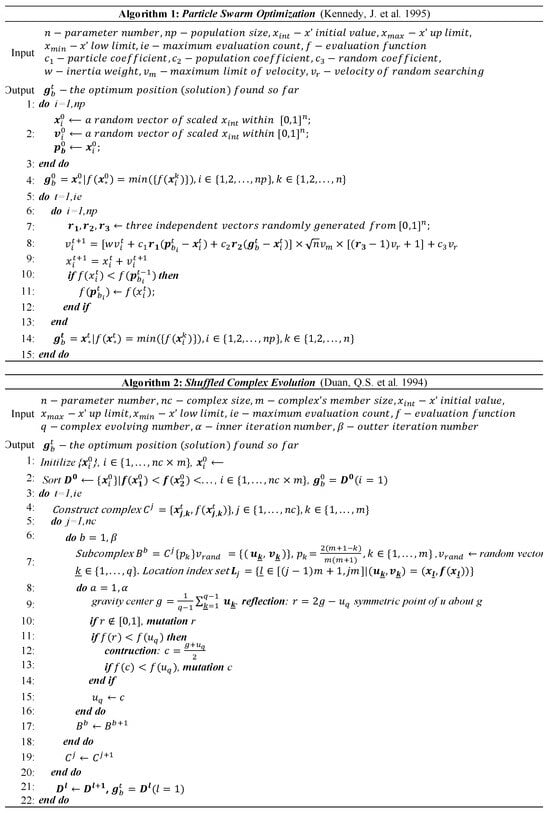
Figure 1.
The pseudo code of the algorithms used in this study [13,14].
Moreover, community and individual social behaviors are incorporated into the core SCE algorithm process [14,65]. The SCE algorithm first randomly selects the scaled (or normalized) parameters () to generate the initial population then further obtains initial local and global optima ( and ) through evaluating and sorting with marked orders at the beginning time (steps 1–2). The following procedures are then repeated until the stop criteria are met. (1) The individuals are evaluated and marked to reorganize the original population into communities, each of which has points (step 4). (2) Complex competitive evaluation (CCE) is conducted for each point to identify the triangular probability distribution [20], known as (step 7), the previous generation is determined, and the new individuals from each community are mixed through reflection and mutation to form a new population (steps 6–17). (3) The individuals are then reordered to form new communities (step 19) and obtain the current local and global optima ( and ) (step 21). Note that and are equal to 2 and , respectively, while the outer cycling number () and the internal and external iteration numbers of CCE ( and ) are equal to , , and , respectively. Therefore, except for and , all other five parameters that can affect the generality of SCE are only related to the dimensions of the LSM parameter space.
Note that is scaled with a threshold normalization equation, i.e., [9,25,26,66,67], for both PSO and SCE. The total individual number () of SCE and total particle number () of PSO both equal . Additionally, for both SCE and PSO, the GSA stops when the evaluation contour () is greater than 105 Noah runs [9]. The equitable population size and stop criteria could ensure the relatively equitable investigation and are intended to reduce the issue that the objective metrics’ impact could be affected by the GSA itself.
2.1.2. Optional Evaluator
The evaluator of the above-mentioned GSA algorithms used in our study is shown in Figure 2, which includes a fixed physical constraint and an optional objective function. The physical constraint formula () represents the soil moisture of the first two surface soil layers ( and , and here in step 2) and only varies between the wilting point (, ) and the soil moisture where transpiration stress begins (, ) [9,16,31].
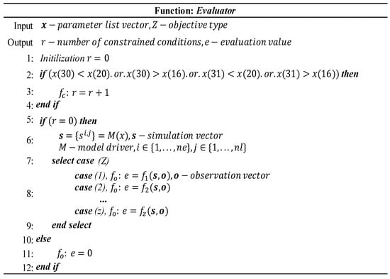
Figure 2.
The pseudo code of the evaluator used in this study.
Under the condition , when constraints are effective, the unscaled parameters will drive the LSM model to run simulation one time for evaluation based on the corresponding objective value, which can be selected based on the objective type (), and is a corresponding constant that varies in [1,8]. Note that once is determined, the predefined corresponding objective metric or function () that measures the distances between simulation and observation is also determined at the very beginning.
2.2. Composited Metrics
For calibration schemes based on GSA, the parameter–simulation problem in the LSM is addressed by searching for the optimal parameters and/or simulations that minimize or maximize the objective function (), which has been extended into multidimensions, i.e., layers () and variables , to meet a holistic SM—ST objective. Nevertheless, the objective indicating the SIM—OBS distance can be quite varied and largely affects the LSM’s complex evaluation [50,51,52,53,54,55,56,57,58,59]. Therefore, eight metric differentiated objectives (Table 1), including the widely used direct measurements (i.e., the correlation and various errors), the composited deterministic measurements (i.e., the various enhanced efficiencies), and the composited flexible measurements (i.e., the Pareto nondominated), are conducted to fulfill the objective metrics’ comprehensive investigation during the present study.

Table 1.
Description of the objective metrics used in this study.
This study mainly examines fixed metrics composed of fundamental measures such as linear correlation coefficient () [58], Kling–Gupta efficiency () [10], absolute error () [57], Nash–Sutcliffe efficiency () [55], and root mean square error () [56] across different dimensions. Specifically, correlation coefficients (CCS), enhanced Kling–Gupta efficiencies (EKGE), mean absolute errors (MAES), Nash–Sutcliffe efficiencies (NSES), and root mean square errors (RMSES) represent the averages of , , , , and across both the variable and layer dimensions. Additionally, the enhanced multiple objectives (EMO) integrate the average values of the measure that combines , , , and in the variable and layer dimensions.
Furthermore, this study has composited various metrics across different dimensions within a non-dominant Pareto space [42,43,50,51] to conduct the Pareto-dominant objective based on the basic land physical laws: that is, since the surface variations of the topsoil layer could often determine the sublayer’s variations through infiltration [24], the dimensional objective of the upper layer is assumed to be the solution. The top layer’s objective that is larger (or smaller) than the sublayers’ is taken as the current optimal maximum (or minimum) solution. Consequently, the Pareto-dominant KGE (PKGE) and the Pareto-dominant multi-objective (PMO) indicate the dominated top layer’s values of EKGE and EMO, respectively.
All the above-mentioned multi-objective metrics’ variable and layer dimensional numbers are 2 and 4, respectively. CCS varies in [−1, 1]. EKGE and NSES both vary in (−∞, 1], and EMO, MAES, and RMSES all vary in [0, +∞). PKGE varies in (−∞, 1], and PMO varies in [0, +∞). Therefore, the value of the metric determines the performance of the evaluator, and the direction of the metric determines the direction of the search, that is, continuously approaching the optimal value of the metric (i.e., the final ideal termination condition) towards the calibrated optimal solution.
2.3. Performance Evaluation
2.3.1. Parameter
During this study, parameter heterogeneity was defined as variations or sensitivities of land parameters across sites. Due to the immense dimensionality of parameter–site sensitivities, parameter relative sensitivities based on the two predefined limits of the parameter space are suggested, e.g., if more (fewer) sites met (failed to meet) a parameter’s limit compared to others, indicating sites’ relative sensitivity to that parameter within the limit’s confidence [9,16]. Since the parameter relative sensitivities (or heterogeneity) are usually large, while their homogeneity could be small (and thus be easily observed), here, to qualify this and simplify the metrics’ diversity investigation, we further propose the parameter numbers with low site sensitivities as homogeneity (H). Consequently, low H (>0) in this study indicates high heterogeneity of one metric quantitatively. Note that when all or no sites cross the parameter’s limits, H equals 0 or , respectively.
The parameter’s spatial uncertainty is defined as the land parameter range and outlier against the sites, e.g., one parameter’s interquartile range (IQR, >0), smaller parameter ranges, and outlier numbers indicated fewer uncertainties and fewer unaccountable factors, respectively fifig9]. In particular, to simplify different metrics’ effects on parameter uncertainty, the whole parameter space’s uncertainty is defined as the interquartile range of all the IQR ensembles of different parameters (or IQRD) in the parameter space. Consequently, the IQRD’s interquartile range and outlier indicate the quantitative parameter uncertainties among metrics.
In particular, compared to SCE, the parameter number with less parameter uncertainties (PNL, >0) and the outlier number reduction of parameter uncertainties (ONR) in PSO are summarized in this study to qualify whether the metrics’ parameter uncertainty is affected by the GSA itself or not. As the heterogeneity and uncertainty differences of different metrics could account for the metric-informed method’s performance in solving parameter spatial complexities during SM—ST calibration, the metric with less parameter uncertainties and heterogeneity could meet the preferable LSM configuration demand in surface forecasting.
2.3.2. Objective
As the population position of a generation, e.g., the best (Pb) or medium (Pm, if non solution is met) locations that are known as fitness against the number of LSM runs (or the convergence speed), could indicate the method’s performance in calibration efficiency, the better fitness values (e.g., larger EKGE values or smaller EMO values) with fewer LSM runs indicate more efficiency, where the success rate exploring evolution abilities is usually put alongside.
Moreover, as the optimal objectives (e.g., the final EKGE or EMO values) could indicate a method’s performance in calibration effectiveness, the larger or smaller optimal objectives that depend on the direction of predefined metrics indicate more effectiveness. Furthermore, since the kernel density distribution of optimal values across different sites demonstrates their spatial enrichment characteristics, the variation in enrichment between different algorithms (such as PSO or SCE) to a certain extent reflects their capacity to address the spatial disparity in SM—ST simulation.
2.3.3. Simulation
To simplify the spatial complexity among regional datasets, linear fitting between the observations (OBS) and simulations (SIM) for all sites is conducted [60]. The linear fitting’s slope (briefed as s hereafter) demonstrates the sensitivity of SIM to OBS, while its coefficient of determination (briefed as r2 hereafter) or the goodness of fit demonstrates if the sensitivity or linear model is robust or not. Moreover, under the assumption of the normal distribution of the errors between SIM and OBS (briefed as hereafter) of all sites, the Gaussian fit of resampled with 100 bins is conducted to generate at most two signals determining the main distribution characteristic., e.g., the amplitude (or frequency, briefed as f hereafter) and center (briefed as c hereafter) [61]. Here, the compound feature of f and c that is closer to the normal distribution indicates better performance or more consistence with the assumption.
The method’s performance in optimal simulation and forecast is qualified using the spatial differences and similarities of surface conditions among different datasets, e.g., surface simulations or reanalysis, and observations, by the following equation:
where and represent the time and the site, respectively, and represents the total number of stations. Smaller and/or high indicate better performance. Note that and are like the formula of the metrics RMSES and CCS (see Table 1) but are conducted within the spatial sequences here.
Meanwhile, the Taylor diagram [52,53,54,55,70], which can assemble the comprehensive statistics (i.e., standard deviation, root mean square difference, and correlation) in a temporal sequence between SIM and OBS, was also created for comparison with the method’s skills. Usually, a smaller distance away from the reference location (i.e., the OBS’s location) indicated more skills. Note that the SIM datasets (30 min) were linearly interpolated into 3 h for a broad comparison with the land reanalysis.
In addition, aside from the uncertainties and heterogeneous requirements in surface prediction parameters (manifested as variations in calibration performance), addressing the precision demands inherent to surface prediction (evidenced by differences in calibration robustness), this study employs indicators such as EKGE increment, reduction, and increment to clarify the performance of various SM—ST objectives in the calibration–forecast framework, aiming to explore the objective metrics’ advantages and/or weaknesses in both the LSM configuration and surface forecasts.
3. Experiments
3.1. Model and Data
The Unified Noah LSM is created to better predict the effects of land surface processes on regional weather, climate, and hydrology. It is intended to comprehend the intricate biophysical, hydrological, and biogeochemical interactions among the soil, the land surface, and the atmosphere at micro- and mesoscales (Figure 3A) [24]. The simple driver Noah LSM (version 3.4.1, https://ral.ucar.edu/model/unified-noah-lsm, accessed on 31 August 2024) has been recently extended into the muti-point applications over central Tibet [9].
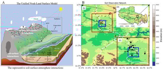
Figure 3.
(A) Noah LSM description. (B) Soil observation network, (a) Tibet and the large scale soil observation network location (box); (b) site locations (filled dots) in the large scale soil observation network, with two types of observation networks (the mesoscale and small scale are in red and blue boxes), roads (white line), and the Naqu city (red asterisk); (c) soil sampling sites (filled dots) in the mesoscale soil network (bold black dots were our study sites).
The SM-ST observations that are firstly derived from the highest altitude soil moisture network in the world (Figure 3B, whose elevations are above 4470 m), which is constructed by the Institute of Tibetan Plateau Research, Chinese Academy of Sciences (ITPCAS) with four soil depths (i.e., 0–5, 10, 20, and 40 cm) [35], are further assembled into the multi-site (i.e., 12) observations of the local warm season (i.e., covering from 1 April to 31 July 2014) over northwest Naqu city, which has a typical semiarid climate, by using simple quality control-based time continuity correction (detailed and described in Ref. [9]). In addition, the global land data assimilation system (GLDAS) [71] grid soil reanalysis data with resolutions of 3 h/0.25° are collected for broader comparison with the surface simulations during this study.
The gridded meteorological surface datasets that merge a variety of data sources were first developed by ITPCAS, with a 3 h interval (3 h) and a resolution of 0.1° × 0.1°, were produced by [72], and are further reassembled into the multi-site LSM forcing dataset by using the inverse distance-weighted quadratic spline interpolation method to drive the Noah LSM.
According to the observational soil and surface characteristics, the multi-site Noah LSM is configured with a four-layer depth and 30 min runtime step, and the soil and vegetation types are mainly silt and grassland, while the slope type is assumed to be flat (e.g., 1). In addition, the forcing time step (3 h) and screen height (i.e., 10 m for winds and 2 m for temperature) for the LSM are the same as the input forcing data [9].
3.2. Experimental Description
A three-month-long warm-up run (covering the period from 1 April to 1 July 2014) of the multi-site LSM, that initialized with the unobserved default parameters (i.e., the “General,” “Vegetation,” “Soil,” and partial “Initial” types) [24,25,26] and partially observational “Initial” parameters (i.e., SMC1-4 and STC1-4), was first conducted to obtain the default multi-site parameter tables, including spatially distinguished “Initial” parameters, for the following experimental runs [9]. Based on this, three types of experiments are conducted, as shown in Figure 4.
Figure 4.
Flowchart of this study. OBS = observations, SIM = simulations, SM = soil moisture, ST = soil temperature, HFX = sensible heat flux, LH = latent heat flux. The superscript * represents the optima of LSM parameter space here.
Following the timeline, (1) a one-month-long run ranging from 1 to 31 July (or the control run, briefed as CTR hereafter) was conducted, as the referenced surface conditions resulted from the default LSM parameter table configuration (). (2) Secondly, the multi-objective metrics varied calibration runs that ranged from 1 to 15 July were conducted to obtain the calibrated multi-site LSM models with metrics-informed parameter tables () and further investigate the metrics’ impact on the calibration’s abilities in solving the spatial complexities of the Noah LSM (e.g., in terms of parameters, objective, and simulations). (3) Finally, the abovementioned various objective-informed LSM models () ranfrom 15 to 31 July to obtain the hopefully improved surface forecasts and further investigate the metrics’ impact on surface forecast (e.g., soil states and surface fluxes).
Following the research flow, (1) the differences between CTR and calibration could account for the calibration performance, and the difference among different calibration runs could account for the metric’s impact on the calibration. (2) Meanwhile, the differences between CTR and calibrated forecast runs could account for the calibrated LSMs’ performances (e.g., in terms of heterogeneity and uncertainty, effectiveness and efficiency, spatial complexities), and the differences among the different calibrated forecast runs should account for the metric’s impact on surface forecast (e.g., in terms of various spatial complexities). (3) After the metrics’ effects on calibration and forecast performances are comprehensively investigated, the best metric configuration of the SM—ST objective in the calibration–forecast framework is finally identified. Notably, all objective metrics within both PSO and SCE algorithms are conducted to explore if the potentially improved surface forecast could be highly affected by the algorithms themselves or not.
In particular, it should be emphasized that this study designs experiments based on the operational scheme of the LSM aiming at improving land surface forecasting. Consequently, the near surface atmospheric forcing conditions (see Section 3.1) in all experiments are identical, meaning that the impact of meteorological forcing on the land surface can be regarded as constant and neglects the surface climate variation factors [73,74]. Thus, the differences observed in the land surface conditions across all experimental results can be attributed solely to the variations in experimental design.
4. Results
4.1. Case Perspective
As land surface models utilize parameters and forcing inputs to prepare land surface forecasts, the issues of surface simulation and local application in typical semi-arid regions (i.e., rapidly applying calibrated parameters to surface forecasts) are exemplified here. To this end, a review of the spatiotemporal characteristics of the default forcing, initial parameters, and their overall simulation status across different periods, including control, simulation calibration, and forecast verification, is conducted to clarify the fundamental manifestations of the issues involved in this study.
4.1.1. Model Configure
The site-averaged 3 h meteorological forcing values against time during the study period are shown in Figure 5a–d. During July 2014, the diurnal variation in temperature () mostly ranged between 5 and 15 °C, with an extremely dry atmosphere in which the relative humidity () values were mostly below 1%. The relatively low wind speed () generally varied between 0 and 6 m s−1, and the wind direction () was mostly dominated by a southern flow (between 180° and 270°) from 1 to 10 July and from 16 to 21 July, respectively, but the opposite in other periods. The incoming shortwave radiation () exhibited strong diurnal variation between 0 and 600 W m−2, and the incoming longwave radiation (L) varied between 250 and 350 W m−2. The pressure () was generally around 586 hPa, and the maximum hourly precipitation () was about 5 mm h−1 on 10 July.
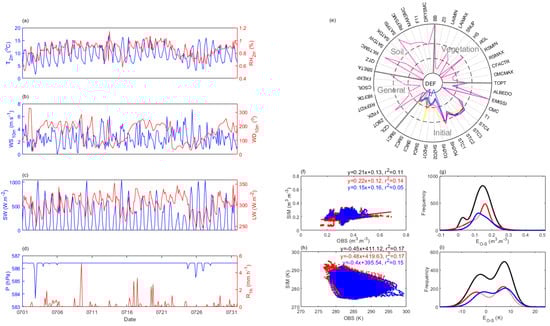
Figure 5.
The case overview in the CTR experiment. (a–d) The meteorological forcing, derived from Ref. [9]. (e) The threshold normalized default parameters of different sites (colored) for calibration. (f,g) The linear and Gaussian fits of the errors between observation and simulation () for of different periods (colored, the whole study period was in black, while the calibration and validation periods were in red and blue, respectively). (h,i) were the same as (f,g), except for .
The initial land parameters of all the sites (or default parameters) that need calibration have shown great variety for the “Initial” types (Figure 5e), and this is especially pronounced for the moisture-related parameters, i.e., the SMC and the SH2O. This should be attributed to the differences in the pre-experiment 3-month simulation of different sites. Furthermore, due to the lack of direct observations for other types of land surface parameters, they are configured using statistical data from optimization experiments based on limited benchmarks from the previous study (serving only as reference inputs for control experiments, consistent with conventional numerical model configurations) [9]. Therefore, in numerical operations, parameter variations among different stations mainly exist in the initial types. Consideration of multi-site calibration can account for the differences among stations with unobserved parameters under existing observational constraints, namely, the spatial heterogeneity and uncertainty of the parameter space. Consequently, the spatial heterogeneity of parameters (i.e., the sensitivity of commonly used parameters to different stations or the number of intersections of the same parameters at different stations in the parameter space) and the characteristics of uncertainty (such as the interquartile range and outlier features of parameters at different stations) in relation to the differences in various optimization objectives are the key areas of focus for further investigation in this study.
4.1.2. Forecast Problem
The CTR simulations and observation datasets for the surface layer are compared in Figure 5f–i. For the whole experimental period, the linear fit for the surface soil moisture (briefed as hereafter) exhibited a small increasing slope (about 0.21) with weak consistency, and the surface soil temperature (briefed as hereafter) had a larger decreasing slope (about –0.45) with strong differences. Moreover, the linear fits of for the calibration and forecast periods were 0.22 and 0.15, respectively, and the linear fits of for the calibration and forecast periods were −0.48 and −0.4, respectively. This indicates that the surface conditions of the forecast period were slightly better than those for the calibration period. Generally, fits better than .
In addition, the ’s for the whole experimental period had a sharp and narrow distribution, which was centered around 0.15 with a frequency of around 800, while the distributions of the calibration and forecast periods had centered around 0.16 and 0.13 , with a frequency of around 500 and 300, respectively. This indicates that values were mostly underestimated for all periods, and this is more pronounced at the calibration period. Nevertheless, the values of for different periods showed bimodal distributions (Figure 5i), whose centers were located around −4 and 9 K (whole period), −5 and 9 K (calibration period), and −4 and 8 K (forecast period), respectively. This indicates that values were both under- and over-estimated, and the latter were more pronounced. Generally, and were both underestimated.
In general, though in CTR exhibited better consistency with OBS than , the overall surface simulation underestimation of the Noah LSM could be great for regional surface forecast applications. Note that either the ITPCAS forcing datasets or the improved heat-sensitive parameter Z0h (also known as CZIL) to improve with the Noah LSM over a surface near our study area [7,75], as well as the non-negligible biased and the spatially diverted parameter space in CTR, indicated a more effective calibration in present study. Since multi-objective calibration can reduce these spatiotemporal errors through parameter identification to improve subsequent forecasts [9], the next focus is on how different objective metrics affect the performance of calibration and forecasting.
4.2. Effects on Calibration
4.2.1. Optimal Parameters
Due to the significant spatial heterogeneity exhibited by most parameters in PSO and SCE, Table 2 has summarized the statistics of H against the four land parameter types during each optimal parameter space for all the experiments, which have been detailed in Figure S1-1, based on the parameter relative sensitivity analysis [9,16,25,26]. For the “Vegetation” type, except for the SCE scenario considering CCS, the H of other scenarios is zero, indicating great heterogeneity. Regarding the “Soil” type, the H values for PSO and SCE calibration schemes (short for Hp and Hs hereafter) based on EKGE, EMO, MAES, and RMSES metrics are (1, 3), (2, 2), (1, 1), and (2, 1), respectively. For the “General” type, the (Hp, Hs) values based on CCS, EKGE, EMO, MAES, and RMSES metrics are (1, A), (2, 2), (2, 2), (1, 1), and (1, 1), respectively. For the “Initial” type, the (Hp, Hs) values based on EKGE, EMO, and MAES metrics are (4, 2), (3, 2), and (2, 1), respectively. Evidently, among all pairs, the spatial homogeneity of optimal parameters for all “Vegetation” types in PSO and SCE is relatively minimal, suggesting the strongest heterogeneity. Conversely, “Soil” and “General” types exhibit minimal spatial heterogeneity, while “Initial” types fall in the middle. Notably, QTZ and SBETA parameters consistently demonstrate homogeneity, below the parameter space threshold (0.33), across PSO and SCE schemes based on EKGE, EMO, MAES, and RMSES metrics.
Table 2.
Parameter spatial homogeneity for all metrics.
Considering the heterogeneity disparities of the entire parameter space among metrics, the H counts of all the parameter types in PSO and SCE are further assembled. For CCS, the counts are 1 and 40, respectively; for EKGE, both schemes yield 7; for EMO, the counts are 7 and 6; for MAES, they are 4 and 3; for NSES, the counts are 2 and none; both PKGE and PMO register none; and for RMSES, the counts are 5 and 2. Evidently, there exist substantial variations in the homogeneity or heterogeneity of the parameters among calibration schemes based on different metrics. Notably, CCS exhibits the lowest parameter heterogeneity, followed by EKGE, then EMO, and subsequently MAES and RMSES. NSES displays relatively poor parameter heterogeneity, whereas PKGE and PMO manifest the highest degree of parameter heterogeneity.
To qualify the metrics’ effect on the parameter uncertainties, both the IQR of each parameter and the IQRD of the entire parameter space contributed by different metrics as shown in Figure 6 are compared. For PSO, the maximum IQR, which has about 4.8 of the parameter SNP in the “Vegetation” type, had the largest uncertainties, while the EMO made the largest contribution. However, the IQR, which is about 1.2 of the SBETA parameter in the “General” type, behaves oppositely, while EKGE, EMO, and RMSES make the smallest contributions (Figure 6a). For SCE, the maximum IQR is around 1.82 of the CZIL parameter in the “General” type, and it has the largest uncertainties, while EMO has the largest contribution. Nevertheless, the IQR that is around 0.61 of the parameter CSOIL in the “General” type behaves conversely, while EKGE, EMO, and RMSES make the smallest contributions (Figure 6b). Generally, PSO achieved higher IQR than SCE for most metrics. PSO and SCE achieved the lowest uncertainties of the parameters SBETA and CSOIL in the “General” type. Moreover, the IQRD of PSO across various metrics exhibits a broader range with more scatters compared to that of SCE (Figure 6c). For PSO, the IQRD median values, ranked from highest to lowest, are PKGE > PMO > NSES > CCS > EMO > EKGE > RMSES > MAES. In contrast, for SCE, the order is PMO > PKGE > EKGE > EMO > MAES > RMSES > CCS. For PSO, the number of outliers in the IQRD is highest for EKGE with 3, followed by EMO and CCS with 2, while the rest of the metrics have zero outliers. For SCE, the EKGE and RMSES numbers of outliers are both 2, followed by EKGE and MAES with 1 outlier each, and the rest are 0 (Figure 6d). In summary, significant differences exist in the IQRD of the entire optimal parameter spaces across different metrics, with SCE exhibiting smaller IQRD but relatively more outliers. Notably, EKGE and EMO exhibit relatively large numbers of outliers in both PSO and SCE.
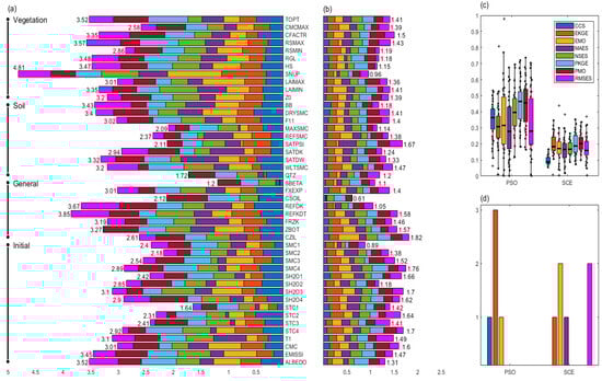
Figure 6.
The different metrics’ parameter spatial uncertainties. (a) The stacked interquartile ranges (IQR, colored) of different optimal parameters for PSO. (b) is the same as (a), but for SCE. (c) The boxplot of the IQR ensembles (or the IQR distributions; IQRD) of the optimal parameter space for various metrics, and their outlier numbers (d). The cross and asterisk represent the extreme and mild outliers respectively.
To qualify the uncertainty’s disparities of different parameter types among metrics that are induced by GSA’s advantages or weakness, Table 3 has summarized the IQR and outlier differences (i.e., PNL and ONR) of different parameter types in the PSO’s optimal parameter space when compared to SCE against different metrics, while the IQR and outliers of both the PSO’s and SCE’s optimal parameter spaces for each metric are detailed in Figure S1-2. For the “Vegetation” type, all metrics are null except for the PNL value of EKGE, which is 2, while the ONR of all metrics is non-positive. For the “Soil” type, the PNL values are positive for all metrics except for CCS, NSES, and PKGE, which are null. The ONR values are positive for EKGE, EMO, PMO, and RMSES while negative for the rest. Regarding the “General” type, all metrics exhibit positive PNL values except for NSES, PKGE, and PMO, whose PNL values are null. The ONR values are positive for EKGE, EMO, MAES, and RMSES and negative for the others. In the “Initial” type, only EKGE and EMO have positive PNL values, with the rest being null. The ONR values are positive for all metrics except for CCS, PKGE, and PMO, which are non-positive. In summary, summing the PNL values across types, EKGE has the highest total (8), followed by EMO and RMSES (7), then MAES (5), with PMO and CCS having the lowest totals (1). PKGE has no PNL value. For the ONR values, EMO has the highest total (9), followed by EKGE (3), then RMSES (3), while PMO has the lowest (2). The rest of the metrics have negative ONR values.
Table 3.
Parameter spatial uncertainties comparison for all metrics.
In general, the overall low homogeneities (e.g., the low H), and the PSO’s low relative advantages (e.g., the general NA PNL with non-positive ONR) have indicated the great parameter heterogeneity and uncertainty challenges and implied higher calibration frequency demand. In particular, the “Vegetation” parameters show the most spatial heterogeneities and uncertainties among all the parameter types, while the “General” type behaves oppositely, which is like the sensitivity tradeoff of the two parameter types over Tibet [7,8,17,22,23]. Moreover, for each objective metric, SCE consistently achieves lower parameter uncertainty than PSO, albeit at the cost of relatively higher spatial heterogeneity, and this tradeoff is in line with the previous study [9]. EKGE and EMO in PSO and EKGE in SCE have yielded the smallest parameter heterogeneities (e.g., low H values), while MAES in PSO and CCS in SCE exhibit the smallest parameter uncertainties (e.g., low IQRD median values). Meanwhile, compared to other metrics, EKGE in PSO and EMO in SCE have shown the most unaccountable factors of the parameter uncertainties, as indicated by having the most outliers of IQRD.
Overall, the “General” and “Vegetation” types have generally shown the opposite tradeoffs in LSM parameter calibration performance in terms of heterogeneity and uncertainty. Once the objective metric is determined, SCE favors lowering parameter uncertainty at the cost of heterogeneity compared to PSO during calibration. EKGE and EMO have shown considerable advantages in reducing parameter heterogeneity compared to other metrics, while the former is slightly more powerful. However, the metrics’ best advantages in reducing parameter uncertainties have shown great diversity (e.g., MAES in PSO and CCS in SCE) and overconfidence (e.g., null accountable factors), while the parameter uncertainty differences of one method induced by metric differences are great (this is especially evident in PSO). This demonstrates that both metric and method could highly affect the parameter uncertainties during calibration.
4.2.2. Effectiveness and Efficiency
Figure 7 shows the different metrics’ fitness curves (i.e., Pb and Pm), and the median position and median Noah run numbers at convergence for different sites, e.g., () and () are for PSO and SCE, respectively. For CCS, both PSO and SCE both sharply increased before 3000 Noah runs, and both converged to 1 but at around 79,475 and 66,663 runs, respectively. For EKGE, PSO and SCE both sharply increased before 10,000 Noah runs but converged to 0.56 at 99,017 runs and 0.53 at 90,731 runs, respectively. For EMO, PSO and SCE both decreased to 1 before 8000 Noah runs but converged to 1 at 99,297 runs and 1.08 at 82,709 runs, respectively. For MAES, PSO and SCE both quickly decreased to the range of 0.7–1.1 before 10,000 Noah runs but converged to 0.79 at 99,765 runs and 0.81 at 94,795 runs, respectively. For NSES, PSO and SCE both instantly reached 1 at 187 runs, indicating the most rapid convergence among all metrics. However, for PKGE and PMO, since volatile finesses (e.g., which vary within and , respectively) are found for all sites in each generation, nonstrict solutions can be observed. For RMSES, PSO and SCE both sharply decreased to 1 before 5000 Noah runs but converged to 0.97 at 99,391 runs and 0.98 at 94,029 runs, respectively.
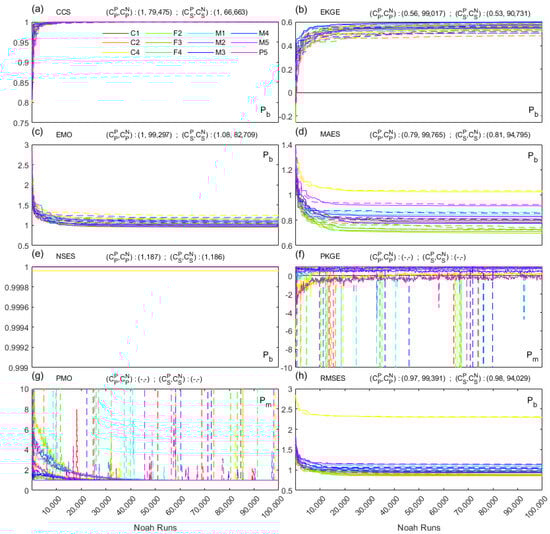
Figure 7.
The different metrics’ impact on calibration effectiveness and efficiency. Fitness curves of different sites (colored) against Noah runs for metrics CCS (a), EKGE (b), EMO (c), MAES (d), NSES (e), PKGE (f), PMO (g), and RMSES (h) in PSO (solid) and SCE (dashed). Except for PKGE and PMO, whose fitness was Pm, others were Pb.
Generally, except for PKGE and PMO, other metrics of PSO achieved better effectiveness, as indicated by their better fitness values, but with relatively worse efficiency, as indicated their larger converged runs compared to those of SCE. The non-solution performance for the metric PKGE and PMO of both PSO and SCE indicated their requirements for more Noah runs in achieving convergence or the potential failure of the Paetro-dominated logic (i.e., that surface improvement likely improves the subsurface). For MAES, NSES, and RMSES, the fitness curve of site C4 is found to be notably biased from (or worse than) that of other sites. Nevertheless, for all the metrics’ convergences, MAES has the largest range, and this could indicate the divergent convergence domain.
Figure 8 presents the success rate curves for calibration across various metrics. For CCS, PSO experiences a decline from 70% to 20% during the first 10,000 Noah runs, followed by a gradual decrease to near zero. In the case of EKGE, PSO initially shows a decline from 80% within the first 5000 Noah runs, subsequently exhibiting two distinct patterns: fluctuations around 40% and 20%, respectively. For EMO, PSO drops from 80% to nearly 0% within the initial 25,000 Noah runs, with some stations subsequently exhibiting strong fluctuations between 0% and 80%. MAES follows a similar trend, with PSO declining from 80% to near 0% within the first 15,000 Noah runs and subsequent intense fluctuations between 0% and 80% at certain stations. For NSES, PSO gradually decreases from 80% to 20% within the first 35,000 Noah runs and remains stable thereafter. PKGE and PMO exhibit similar behavior, with PSO slowly declining from 80% to 20% within the first 20,000 Noah runs and fluctuating slightly around 20% thereafter. SCE’s performance in PKGE resembles that of CCS. In contrast, RMSES displays a fluctuating decline from 80% to 0% within the initial 20,000 Noah runs for PSO, followed by drastic fluctuations between 20% and 80%. However, SCE consistently demonstrates a rapid initial decrease from 80% to 20% across nearly all metrics, maintaining this level thereafter.
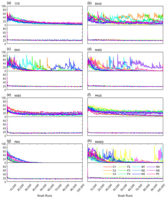
Figure 8.
Success rate curves of different sites (colored) against Noah runs for metrics CCS (a), EKGE (b), EMO (c), MAES (d), NSES (e), PKGE (f), PMO (g), and RMSES (h) in PSO (top) and SCE (bottom).
For all metrics, the search domain of SCE exhibits a consistent pattern, characterized by an L-shaped thin linear region. In contrast, PSO’s search domain displays significant fluctuations and notable variations across different metrics (e.g., EKGE, EMO, MAES, RMSES), albeit with an overall larger area than SCE. This suggests that for most metrics, PSO demonstrates stronger evolutionary capabilities compared to SCE, which primarily contributes to PSO’s slightly slower convergence rate compared to SCE.
Figure 9 presents the statistical performance of the optimal objectives across all stations for various metrics. For CCS, both PSO and SCE exhibit a concentrated distribution near 1, with PSO displaying a tighter clustering and an outlier at 0.973. In the case of EKGE, PSO and SCE concentrate around 0.58 and 0.53, respectively, with PSO showing a more focused distribution and an outlier at 0.34. For EMO, PSO and SCE are centered near 1 and 1.1, respectively, with PSO displaying a relatively dispersed distribution and an outlier at 1.5. MAES values for PSO and SCE are centered around 0.79 and 0.81, respectively, demonstrating similar distributions. For NSES, PKGE, and PMO, both PSO and SCE have concentrated distributions near 1, with NSES exhibiting a more tightly clustered distribution compared to the other two metrics. Finally, for RMSES, PSO and SCE are centered around 0.9 and 1.1, respectively, with SCE displaying a more focused distribution and both having outliers at around 2.4.

Figure 9.
The different metrics’ impact on optimal objective uncertainties against sites for PSO and SCE. The asterisk represents for the outlier.
It is evident that for the optimal solutions of PKGE and PMO, both PSO and SCE yield values of 1, indicating the absence of optimal solutions or the need for more time to locate them. In contrast, numerical optimal solutions were achieved for other metrics. Furthermore, while PSO consistently outperformed SCE in attaining better optimal solutions across almost all metrics, significant variations were observed in the enrichment levels of optimal solutions between PSO and SCE under different metrics. For instance, PSO surpassed SCE in CCS and EKGE, whereas SCE surpassed PSO in EMO, MAES, and RMSES. Notably, PSO and SCE exhibited similar performance in NSES. This underscores the disparate spatial variability characteristics of optimal solutions influenced by distinct metrics (whereby the enrichment levels of optimal solutions at different sites reflect the extent of spatial variability or heterogeneity). Additionally, notable outliers were identified in PSO’s performance within CCS, EKGE, and EMO metrics, while both PSO and SCE exhibited outliers in the RMSES metric. This indicates that for RMSES, unquantifiable factors within the spatial variability of optimal solutions are more pronounced, whereas for other metrics, PSO’s performance relative to SCE is more significantly influenced.
Overall, apart from PKGE and PMO, for other metrics, PSO typically exhibits better optimal solutions, i.e., enhanced effectiveness, compared to SCE, albeit at the cost of relatively lower efficiency. Notably, for CCS, EKGE, and RMSES, the optimal solutions obtained by PSO demonstrate higher kernel densities (or lower spatial variability) than those obtained by SCE, while for EMO and RMSES, the performance behaves oppositely, and for other metrics, kernel densities of optimal objectives are almost equal. In particular, only these enrichment advantages resulting from metrics such as CCS, EKGE, and RMSES in PSO have commonalities of the positive PNL in the “General” type (Table 3), which likely indicate the “General” type’s advantages in lowering the spatial variabilities of calibration objectives [15,16,17]. However, recall that the overall PNL values are much smaller than the LSM parameter dimensions (Table 2 and Table 3), and the optimal objective’s absorption resulting from parameter advantages could be small, while their resulting simulation differences need further investigation.
4.2.3. Optimal Simulation
Linear and Gaussian Fitting
Figure S2-1 presents linear fitting, whose indicators are slope and goodness of fit (briefed as (s,r2) hereafter), between simulations and observations for and under varying metrics. For , the PSO’s s values (in descending order) are EMO, EKGE, RMSES, MAES, PMO, NSES, CCS, PKGE, with r2 values also descending from EMO to PKGE. In contrast, the order of SCE s values is EMO, PMO, EKGE, MAES, PKGE, NSES, RMSES, and CCS, with r2 following a similar but slightly different descending order. For ’s linear fitting (Figure S2-1-2), the PSO s values are, in order, EKGE, EMO, MAES, RMSES, CCS, NSES, PKGE, PMO, while r2 values show a distinct ordering: PMO, followed closely by EMO and PKGE, then with MAES, RMSES, and NSES closely grouped, then EKGE, and finally CCS. SCE fitting for exhibits a different ordering for s (EKGE, EMO, CCS, RMSES, MAES, NSES, PMO, PKGE) and r2 values (PKGE, PMO, NSES, EKGE, EMO, RMSES, with CCS and MAES closely grouped).
Generally, for , except for metrics like NSES, PKGE and PMO in both PSO and SCE exhibit negative s values, while the rest are positive (Table 4). This indicates that most linear relationships between calibrated simulations and observations are positively correlated, which aligns with the improvement objectives of this study. Specifically, for EMO and EKGE, the s values of PSO (SCE) in the calibration of and are 0.96 (0.83) and 0.18 (0.23), respectively, showcasing the optimal calibration performance (Figure 10). Furthermore, it is noteworthy that for , the highest r2 value of 0.11 is comparable to the lowest r2 value observed in (PKGE), implicitly suggesting a greater challenge in modeling .
Table 4.
Linear fits between surface soil simulations and observations against sites for all metrics.

Figure 10.
Different metrics’ best linear fits against sites for (a) and (b) during the calibration period. CRT, PSO, and SCE are plotted in black, red, and blue, respectively.
The Gaussian fitting, with indicators of center and frequency (briefed as (c, f) hereafter), of for in Figure S2-2-1 reveals the following: CTR is widely distributed, peaking at ~0.15 (f = 297). In PSO and SCE, CCS values span widely around −0.04 (f ≈ 350) and 0.11 (f ≈ 295), EKGE narrowly centers at 0 (f ≈ 1276) and 0 (f ≈ 608), EMO narrowly peaks at 0 (f ≈ 1178) and 0.01 (f ≈ 700), MAES widens slightly at 0.01 (f ≈ 344) and 0.02 (f ≈ 416), NSES values are wide at 0.05 (f ≈ 274) and 0.05 (f ≈ 230), PKGE widely centers at 0.08 (f ≈ 322) and 0.11 (f ≈ 325), PMO narrowly peaks at 0.02 (f ≈ 480) and 0.03 (f ≈ 444), and RMSES narrowly centers at −0.02 (f ≈ 426) and 0 (f ≈ 296). Moreover, the c (f) of for (Figure S2-2-2) shows the following: CTR has a wide bimodal distribution centered at ~7.1 (f ≈ 192) and −3.8 (f ≈ 134). In PSO and SCE, CCS widely centers at ~2.3 (f ≈ 216) and 1.1 (f ≈ 167), EKGE widely centers at ~1.3 (f ≈ 200) and 2.5 (f ≈ 203), EMO centers at ~0.85 (f ≈ 170) and 1.23 (f ≈ 207), MAES centers at ~−0.06 (f ≈ 200) and 0.88 (f ≈ 230), NSES widely centers at ~5.86 (f ≈ 169) and 5.03 (f ≈ 213), PKGE widely centers at ~4.91 (f ≈ 237) and 5.01 (f ≈ 152), PMO widely centers at ~6.1 (f ≈ 300) and 5.19 (f ≈ 224), and RMSES centers at ~0.16 (f ≈ 200) and 1.29 (f ≈ 206).
Generally, for of , EKGE’s performance in both PSO and SCE is closest to a normal distribution, whereas for that of , MAES exhibits the closest resemblance to normality (Figure 11), with EKGE performing relatively poorly (Table 5). This underscores the significant influence of metric discrepancies on optimal simulation errors, contingent upon distinct calibration objectives. Furthermore, excessively wide peaks with low frequencies in unimodal distributions (e.g., CCS, NSES, PKGE, and PMO) indicate the dispersed fitting distribution, potentially necessitating the multimodal (e.g., more than two peaks) fitting. Conversely, bimodal distributions characterized by narrower peaks may call for a single-peak fitting.
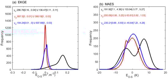
Figure 11.
Different metrics’ best Gaussian fits of against sites for (a) and (b) during the calibration period. CRT, PSO, and SCE are plotted in black, red, and blue, respectively. In addition, the two typically characterized “amplitudes [peak position, peak width]” in Gaussian fitting are displayed together. Note that two amplitudes with one identical peak could be summed to one amplitude.
Table 5.
Gaussian fits of of surface soil simulations against sites for all metrics.
In general, EMO, EKGE, and PMO have slopes greater than 0.7, showing promising linear modeling, while EKGE, EMO, MAES, and RMSES have slopes greater than 0.1, showing better linear modeling than other metrics. Furthermore, EKGE and EMO have unbiased errors centered around 0 for , showing promising nonlinear modeling, while MAES, RMSES, and EMO have unbiased errors centered around 1, showing better nonlinear modeling than other metrics, e.g., EKGE is biased around 3 K. Overall, EMO has shown the most advantages in surface soil modeling among all metrics.
Spatial Difference and Similarity
Figure 12a depicts temporal variations for . CTR is generally the largest, at 0.15 (decreasing during 5 and 10 July rainfalls), followed by a slight upward trend. For CCS, PSO slightly fluctuates between 0.1 to 0.17, while SCE fluctuates around 0.07. EKGE and EMO values in PSO (SCE) are around 0.01 (0.03) and 0.01 (0.02), respectively, both trending downward. MAES values in both PSO and SCE are around 0.04, both declining. NSES values in both PSO and SCE are around 0.07, upward trending. PKGE in PSO (SCE) is 0.12 (0.1), upward trending. PMO in PSO decreases from 0.1 to 0.05, while SCE values are around 0.07, slightly decreasing. RMSES values in PSO (SCE) are 0.04 (0.05), both declining. Moreover, Figure 12b illustrates the overall distribution for . Median values ranking from highest to lowest for PSO are as follows: CCS (0.13) > PKGE (0.12) > NSES (0.08) > PMO (0.07) > RMSES (0.039) > MAES (0.038) > EMO (0.018) > EKGE (0.017); for SCE: PKGE (0.1) > CCS (0.09) > NSES (0.085) > PMO (0.065) > RMSES (0.056) > MAES (0.039) > EKGE (0.03) > EMO (0.02). Notably, EKGE in PSO and EMO in SCE exhibit the lowest median , whereas CCS in PSO and PKGE in SCE have the highest.
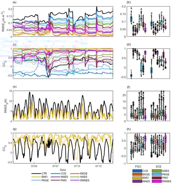
Figure 12.
The different metrics’ impact on the optimal surface simulation. (a) The temporally varied and (b) the boxplot of for . (c,d) are the same as (a,b) but showing the for . (e–h) are the same as (a–d), but for , note that only the best metric performance is shown in (e,g) to avoid overlaps. The cross and asterisk represent the extreme and mild outliers respectively.
Figure 12c depicts temporal variations of the of . CTR significantly drops 5–6 July (0.5 to −0.6), fluctuating at ~0.2 otherwise. For CCS, PSO is stable at −0.5, and SCE increases 5 July (−0.4 to 0.5) then sharply drops to −0.2. For EKGE, PSO and SCE fluctuate around 1 and 0.8. For EMO, both are ~1. For MAES, PSO increases (0.2 to 1), SCE initially declines 4–5 July (0.4 to 0) and then becomes ~0.2. For NSES, PSO ~0.7 and then drops post 10 July to ~0.5; SCE ~0.2. For PKGE, PSO ~0.45, with a sharp drop 5 July to ~−0.4; SCE is −0.4, with a sharp increase 4 July to 0.5, followed by a sharp drop 6 July to ~−0.3. For PMO, PSO is 0.6, with a sharp drop 6 July to −0.5, followed by a rise to 0.2; SCE is 0.8 then drops 5 July to 0 and rises to 0.4. For RMSES, PSO increases (0.5 to 0.8) and stabilizes ~0.8 post 4 July; SCE is ~0.45, declines 4–6 July, and rises to ~0.26. EMO and EKGE consistently outperform MAES for PSO and SCE, with other metrics displaying varied trends. Moreover, Figure 12d illustrates the overall distribution for . Median values, ranking from highest to lowest for PSO, are as follows: EMO > EKGE > MAES > RMSES > NSES > PMO > PKGE > CCS; for SCE: EKGE > EMO > MAES > PMO > PKGE > NSES > RMSES > CCS. Notably, EMO in PSO and EKGE in SCE exhibit the highest median , whereas CCS in PSO and SCE has the lowest.
For of , CTR shows a marked diurnal variation, averaging 8 K fluctuations (Figure S2-3-1). Due to overlapping diurnal error ranges, its performance complexity surpasses . Notably, NSES, PKGE, and PMO peak values > 14 K (CTR’s max), indicating inferiority (Figure 12e). Conversely, MAES and RMSES peak at 8 K, surpassing CTR. EKGE and EMO, excluding initial days, also peak near 8 K, outperforming CTR. Median (K) values ranking from highest to lowest yields the following order for PSO: PMO (7.5) > PKGE (6) > NSES (5.8) > CCS (4) > EKGE (3.5) > MAES (2.8) > RMSES (2.5) > EMO (2.48); and for SCE: PKGE (6.1) > PMO (5.8) > NSES (5.6) > CCS (3.6) > EKGE (3.3) > MAES (2.9) > RMSES (2.7) > EMO (2.5) (Figure 12f). EMO in both PSO and SCE exhibits the lowest median , whereas PMO in PSO and PKGE in SCE possess the highest.
Furthermore, for of , CTR varies from −0.5 to 0.7, showing distinct diurnal patterns (Figure 12g). Overlapping diurnal error ranges complicate performance compared to (Figure S2-3-2). In both PSO and SCE, CCS and EKGE maximums are less than 0.7 (CTR’s max), indicating inferiority, while NSE, PKGE, and PMO maximums rival CTR, but minimums are larger than −0.5, outperforming CT; EMO, MAES, and RMSES maximums are around 0.8, exceeding CTR. Hence, performance ranks EMO, MAES, and RMSE as the best, followed by NSE, PKGE, and PMO; CCS and EKGE perform badly. Moreover, Figure 12h illustrates the overall distribution of . Median values ranking from highest to lowest for PSO are as follows: EMO > MAES > RMSES > NSES > PMO > PKGE > EKGE > CCS; for SCE: EMO > RMSES > CCS > EKGE > MAES > PKGE > PMO > NSES. Notably, EMO exhibits the highest median for both PSO and SCE, whereas CCS and NSES have the lowest.
Overall, for , EKGE in PSO and EMO in SCE have the lowest median when EMO in PSO and EKGE in SCE have the highest median , which shows the complex triangular tradeoffs among metrics, algorithms, and simulation complexities. Nevertheless, for , EMO in both PSO and SCE exhibits the lowest median and the highest median , which demonstrate the significant benefits of EMO in reducing simulation complexities. Generally, for , EKGE in PSO and EMO in SCE have the best and performances, respectively, while for , EMO in both PSO and SCE has the best and performances. It is noted that the EMO’s general advantages of solving the optimal simulations’ complexities are likely in line with its advantages in reducing parameter heterogeneities (Table 2).
4.3. Effects on Forecast
4.3.1. Linear and Gaussian Fitting
Figure S3-1 illustrates disparities in linear fitting (s, r2) between simulations and observations for and across metrics. For ‘s linear fit (Figure S3-1-1), PSO’s s values (descending) are as follows: EKGE > EMO > MAES > RMSES > NSES > PMO > CCS > PKGE; the r2 order matches. For SCE, s values in descending order are as follows: EMO > EKGE > PMO > MAES > NSES > RMSES > CCS > PKGE. The r2 order differs: EKGE > EMO > MAES > PMO > NSES > PKGE > RMSES > CCS. For ’s fit (Figure S3-1-2), PSO’s s values are in order as follows: MAES > RMSES > EMO ≥ EKGE/CCS > NSES > PKGE > PMO; for r2, the order is as follows: PMO > PKGE > EMO > RMSES ≥ MAES/NSES > EKGE > CCS. SCE’s s values are in the following order: MAES/CCS > RMSES > EMO/EKGE > NSES > PMO > PKGE; for r2, the order is as follows: PKGE > RMSES/PMO > MAES/EMO > NSES > CCS/EKGE.
Generally, in addition to of NSES, PKGE, and PMO and of PKGE, both PSO and SCE exhibit positive s values (Table 6). This indicates that the forecasts and observations are positively correlated. Specifically, for of EKGE and of MAES, the s (r2) values of PSO (SCE) and are 0.98 (0.84) and 0.14 (0.15), respectively, showcasing the best performance (Figure 13). Furthermore, it is noteworthy that for of MAES, the highest r2 value of 0.1 is much smaller than the highest r2 value observed for of EKG, implicitly suggesting a greater challenge in forecasting.
Table 6.
Linear fits between surface soil simulations and observations against sites for all metrics.
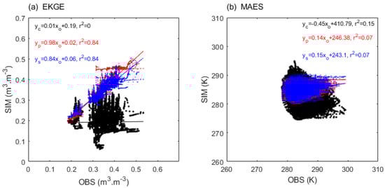
Figure 13.
Different metrics’ best linear fits against sites for (a) and (b) during the forecast period. CRT, PSO, and SCE are plotted in black, red, and blue, respectively.
The c (f) values of of (Figure S3-2-1) reveal the following: CTR centered at 0.19 (f ≈ 272). In PSO and SCE, the CCS centers are at 0.15 (f ≈ 189) and 0.07 (f ≈ 225), EKGE narrowly centers at 0 (f ≈ 383) and 0 (f ≈ 363), the EMO centers are at 0 (f ≈ 416) and 0 (f ≈ 359), the MAES centers are at −0.01 (f ≈ 359) and 0 (f ≈ 284), NSES centers at 0.06 (f ≈ 343) and 0.05 (f ≈ 322), PKGE bimodally centers at 0.13/0.04 (f ≈ 234/220) and 0.16/0.06 (f ≈ 199/365), PMO widely centers at 0.01 (f ≈ 367) and 0.04 (f ≈ 323), and RMSES centers at −0.02 (f ≈ 293) and 0.01 (f ≈ 326). Furthermore, the c (f) values of of (Figure S3-2-2) reveal the following: CTR bimodally centers at 7.28/−3.57 (f ≈ 211/160). In PSO and SCE, CCS widely centers at 3.2 (f ≈ 187) and −0.38 (f ≈ 181), EKGE centers at −0.09 (f ≈ 143) and 3.39 (f ≈ 189), EMO centers at −1.41 (f ≈ 175) and −0.98 (f ≈ 148), MAES centers at 0.49 (f ≈ 181) and 0.29 (f ≈ 206), NSES widely centers at 5.81 (f ≈ 204) and 4.56 (f ≈ 210), PKGE widely centers at 4.9 (f ≈ 214) and 5.7 (f ≈ 217), PMO widely centers at 6.17 (f ≈ 221) and 5.47 (f ≈ 187), and RMSES centers at 0.55 (f ≈ 194) and 0.32 (f ≈ 198).
Generally, for of , EMO and EKGE in both PSO and SCE are closest to the normal distribution, whereas for that of , MAES exhibits the closest resemblance to normality (Figure 14), with EKGE in SCE having a positive bias around 3.3 K (Table 7). The unbiased errors of for EKGE and EMO and the unbiased errors of for MAES are consistent with the surface modeling advantages indicated by the linear fitting. Nevertheless, the metrics’ inconsistences of the best Gaussian fitting of errors in calibration and forecast underscore the significant influence of metric discrepancies on forecast errors. Furthermore, excessively wide peaks with low frequencies in unimodal distributions (e.g., CCS, NSES, PKGE, and PMO), which is consistent with the optimal simulations’ Gaussian fitting (see Section 4.2.3), indicate the dispersed fitting distribution, potentially necessitating the multimodal (more than two peaks) fitting.
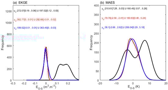
Figure 14.
Different metrics’ best Gaussian fits of against sites for (a) and (b) during the forecast period. CRT, PSO, and SCE are plotted in black, red, and blue, respectively. In addition, the two typically characterized “amplitude [peak position, peak width]” values in Gaussian fitting are displayed together. Note that two amplitudes with one identical peak could be summed to one amplitude.
Table 7.
Gaussian fits of of surface soil simulations against sites for all metrics.
In general, EMO and EKGE have slopes greater than 0.8, showing promising linear modeling, while EMO, MAES, and RMSES have slopes greater than 0.1, showing better linear modeling than other metrics. Furthermore, EKGE and EMO have unbiased errors centered around 0 for , showing promising nonlinear modeling, while MAES, RMSES, and EMO have unbiased errors centered around 0.3, 0.3, and −1, showing better nonlinear modeling than other metrics, e.g., EKGE is biased around 3 K. Overall, EMO has shown the most advantages in surface soil modeling among all metrics. This is consistent with EMO’s surface modeling performance during the calibration period (see Section 4.2.3 on “Linear and Gaussian Fitting”).
4.3.2. Spatial Difference and Similarity
Figure 15a depicts the temporal variations of . CTR is largest (~0.15), fluctuating with a dip on 24 July. CCS in PSO ranges around 0.13 then trends upward, while it remains stable at 0.1 in SCE. EKGE and EMO in PSO/SCE are ~0.02/0.01 and ~0.02/0.02, respectively, with both trending slightly upward. In both PSO and SCE, MAES values are ~0.04, NSES hovers at 0.07 with a slight decline, PKGE is ~0.12, and PMO declines from ~0.07 to 0.0. RMSES values in PSO/SCE are ~0.04/0.06. Furthermore, Figure 15b illustrates the overall distribution of . The median values ranking from highest to lowest for PSO are as follow: CCS (0.12) > PKGE (0.11) > NSES (0.07) > PMO (0.05) > MAES (0.04) > RMSES (0.036) > EMO (0.028) > EKGE (0.02); for SCE, PKGE (0.11) > CCS (0.1) > NSES (0.07) > RMSES (0.052) > PMO (0.05) > MAES (0.04) > EMO (0.02) > EKGE (0.019). Notably, EKGE has the lowest median for both PSO and SCE, whereas CCS in PSO and PKGE in SCE have the highest.
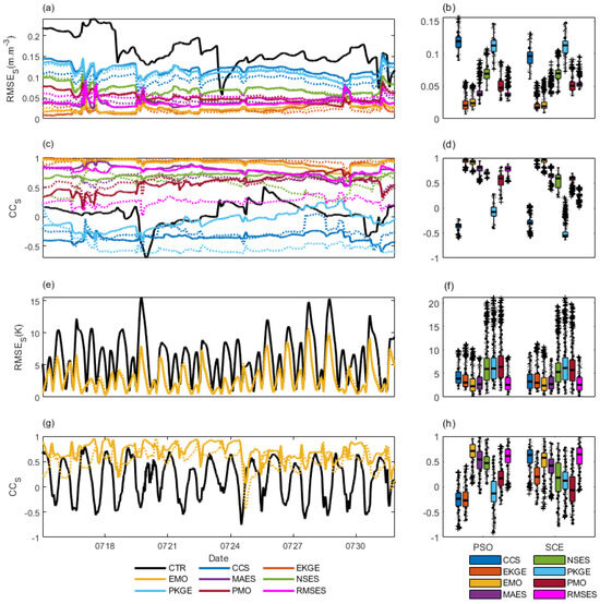
Figure 15.
The different metrics’ impact on the soil forecast. (a) The temporally varied and (b) the boxplot of of . (c,d) are the same as (a,b) but showing of . (e–h) are the same as (a–d), except for , note that only the best metric performance is shown in (e,g) to avoid overlaps. The cross and asterisk represent the extreme and mild outliers respectively.
Figure 15c shows temporal variations of . CTR significantly drops from 20–21 July (0.1 to −0.7) and is stable at ~0.2 otherwise. In both PSO and SCE, CCS hovers around −0.3. EKGE in PSO remains ~0.8, while in SCE, it jitters at ~0.3. EMO is ~1 in both PSO and SCE. MAES in PSO is ~0.8, declining gradually, while in SCE, it drops from 0.4 to 0 (5 July) and then rises slightly to ~0.2. NSES in PSO starts at 0.7, dropping to ~0.5 post 10 July; while in SCE, it jitters at ~0.2. PKGE in PSO is ~0.45, sharply dropping to ~−0.4 post 5 July, while in SCE, it initially is ~−0.4 then jitters at ~−0.3. PMO in PSO starts at ~0.6, sharply drops to ~−0.5 (6 July), and rises to ~0.2, while in SCE, it starts at ~0.8, drops to 0, and rises to ~0.4. RMSES in PSO jitters and rises (0.5 to 0.8), stabilizing at ~0.8 post 4 July, while SCE starts at ~0.45, drops to ~0 (4–6 July), and rises, fluctuating around ~0.26. For of , PSO and SCE consistently rank in the order EMO > EKGE > MAES, with the others exhibiting unstable/inferior performance. Figure 15d depicts the overall distribution of . The median ranking from highest to lowest, for PSO, is as follows: EKGE > EMO > MAES > RMSES > NSES > PMO > PKGE > CCS; for SCE, it is as follows: EKGE > EMO > MAES > PMO > NSES > RMSES > PKGE > CCS. Notably, EKGE has the highest median for both PSO and SCE, while CCS has the lowest.
Figure 15e displays temporal variations of . CTR exhibits pronounced diurnal fluctuations at 10 K. Metric performances are intricate due to overlapping diurnal error amplitudes (Figure S3-3-1). In both PSO and SCE, NSES, PKGE, and PMO maximums exceed 15 K (CTR’s max), indicating inferior performance, while EMO, MAES, and RMSES maximums are lower than 7 K, superior to CTR. Noted that CCS and EKGE maximums in both PSO and SCE are around 8K (except 1–2 July), also outperforming CTR. For of , in both PSO and SCE, EMO, MAES, and RMSES show as the smallest, followed by CCS and EKGE, while NSES, PKGE, and PMO are the highest. Moreover, Figure 15f shows the distribution of . Median values ranking from highest to lowest, for PSO, are as follows: PMO (7.5) > PKGE (6.9) > NSES (6.6) > CCS (4) > EKGE (3) > RMSES (2.9) > MAES (2.7) > EMO (2); for SCE: PKGE (7) > PMO (6.8) > NSES (6.4) > CCS (3.8) > EKGE (3.3) > MAES (2.7) > RMSES (2.5) > EMO (2.3). EMO in both PSO and SCE has the lowest median , whereas PMO in PSO and PKGE in SCE have the highest.
Figure 15g presents temporal variations of . CTR displays strong diurnal fluctuations between −0.7 and 0.7. Overlapping diurnal error amplitudes complicate performance (Figure S3-3-2). Notably, EMO, MAES, and RMSES in both PSO and SCE exceed CTR’s extremes, demonstrating superior performance. Moreover, Figure 15h depicts the overall distribution of . The median ranking from highest to lowest, for PSO, is as follows: EMO > RMSES > MAES > NSES > PMO > PKGE > CCS > EKGE; for SCE: RMSES > CCS > EMO > MAES > EKGE > NSES > PKGE > PMO. Notably, EMO in PSO and RMSES in SCE have the highest median , while EKGE in PSO and PMO in SCE have the lowest.
Overall, for , EKGE in both PSO and SCE has the lowest median and the highest median , whereas CCS and PKGE behave oppositely. For , EMO in both methods has the lowest median , whereas PMO in PSO and PKGE in SCE have the highest. In addition, EMO in PSO and RMSES in SCE have the highest median , while EKGE in PSO and PMO in SCE have the lowest. Generally, for , EKGE has the best and performances, while for , EMO in PSO and RMSES in SCE have the best and performances, respectively. Nevertheless, EMO has shown no weakness performance, while EKGE in PSO has the lowest similarity for , which is consistent with the EMO’s advantages during the calibration period (see Section 4.2.3 on “Spatial Difference and Similarity”).
4.3.3. Surface States Intercomparison
Figure 16 presents Taylor diagram plots of calibrated and CTR simulations of during the forecast period, compared with observations and/or GLDAS data, across various metrics. For the comparison of simulations with observations (Figure 16a), CTR exhibits a root mean square difference () greater than 0.02, surpassing other simulated metrics and GLDAS. However, the correlation coefficient () between CTR and observations is above 0.5, outperforming other simulations and GLDAS except for EKGE and EMO metrics. Additionally, CTR’s standard deviation () reaches approximately 0.03, significantly higher than that of other simulated metrics and GLDAS. Thus, EKGE and EMO metrics, when applied in PSO and/or SCE, effectively improve the simulation of . In the comparison of with observations (Figure 16b), CTR, GLDAS, and multiple simulations demonstrate no skill. Nevertheless, like , simulations using EKGE and EMO metrics consistently yield the lowest and , as well as the highest among all evaluated metrics.
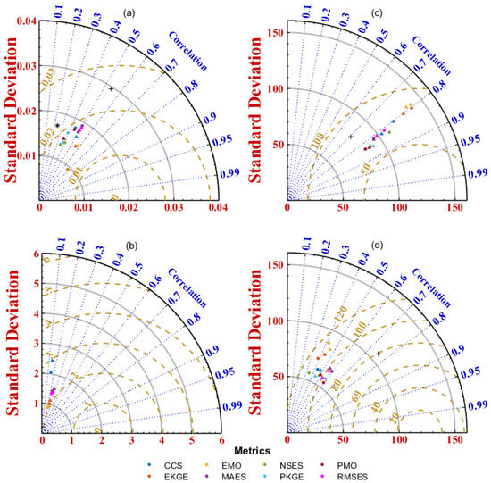
Figure 16.
The different metrics’ impact on surface forecast. (a,b) The Taylor diagram against observations for and , respectively, and the CTR and GLDAS are shown in cross and asterisk markers, respectively, while PSO and SCE are shown in circles and triangles, respectively. (c,d) The Taylor diagram against GLDAS for HFX and LH, respectively, and the CTR values are shown in cross markers.
Furthermore, for the comparison of sensible heat flux (HFX) with GLDAS (Figure 16c), CTR displays higher and lower than other simulated metrics, albeit with a relatively low . This suggests that while most other metrics’ HFX simulations outperform CTR in terms of and , their values are relatively increased, with EKGE and EMO ranking as the top two in both PSO and SCE for . In contrast, for the comparison of latent heat flux (LH) with GLDAS (Figure 16d), CTR exhibits lower and higher than other simulated metrics but with a relatively high . Notably, CTR’s LH simulation surpasses other metrics in both and . Specifically, EKGE and EMO rank as the top two for both and in both PSO and SCE, which is a notable contrast to the findings for HFX.
Overall, for and , EKGE and EMO exhibit high Taylor diagram skills (briefed as TDS hereafter) in both PSO and SCE, significantly outperforming CTR. However, when compared with GLDAS, the TDS of HFX for all metrics in both PSO and SCE is superior to CTR, whereas the performances of LH show the opposite. Evidently, the enhancement of surface soil moisture and temperature simulations often yield more divergent surface flux simulation, indicating either the high complexity of modeling both the surface states and the surface fluxes in arid regions or the biased LH in GLDAS.
4.4. Configure and Benefit
Figure 17 compares the parameter ranges of the “best metric’s simulations” between PSO and SCE, alongside the values of various metrics for surface soil moisture simulations against observations. It is observable that in PSO, the optimal parameter range of EMO is larger than that of EKGE, whereas the opposite holds true for SCE, where EMO’s optimal parameter range is smaller than EKGE’s (Figure 17A). The values of from optimal simulations of different metrics indicate that in PSO, EKGE achieves the highest value, whereas in SCE, EMO attains the peak (Figure 17a). For , however, EKGE’s optimal simulation yields the highest value in both PSO and SCE (Figure 17c). In terms of forecasted , EKGE consistently produces the highest values in both PSO and SCE (Figure 17b). Conversely, for , CCS achieves the highest values in both PSO and SCE, with EKGE following closely (Figure 17d).
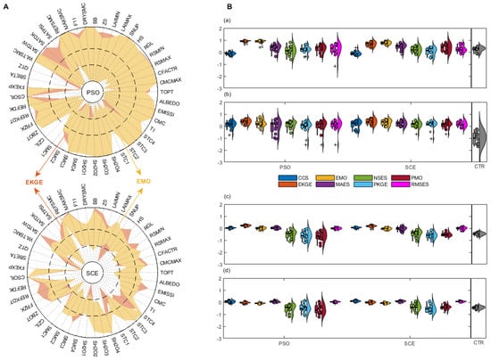
Figure 17.
The best LSM parameters’ configuration (A), and the different metrics’ impact on the indicators of surface simulation (B) in PSO and SCE. Among B, (a,b) represent the discrete distribution (box and scatter) and its density (ridge) of of the calibration and forecast periods, respectively, for , while (c,d) are the same as (a,b), but for . Note that all the metrics’ performances are shown in color that align with the legend except CTR in grey.
Figure 18 illustrates the changes in reductions and increases of the simulations for various metrics and CTR during the calibration and validation periods. For , during the calibration period, most metrics, except CCS, exhibit a reduction in compared to CTR, with EMO and EKGE showing the most significant improvements (Figure 18a), which is also reflected in their highest (Figure 18e). During the validation period, EKGE and EMO stand out among the metrics, excluding CCS and PKGE, in terms of reduction (Figure 18b), again accompanied by the highest (Figure 18f). For , during the calibration period, reductions relative to CTR are observed for most metrics except PKGE, PMO, and NSES, with MAES, RMSES, and EMO demonstrating the most pronounced improvements (Figure 18c), which also correspond to the highest (Figure 18g). Similarly, during the validation period, reductions are observed for most metrics except PKGE, PMO, and NSES, with MAES, RMSES, and EMO continuing to show the most significant improvements (Figure 18d), accompanied by the highest (Figure 18h).
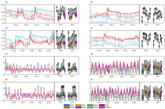
Figure 18.
The different metrics’ impact on the LSM’s spatial difference reduction and similarity increment. (a) Time-varied reduction (PSO, solid; SCE, dotted) compared to CTR (left) and the box-plotted reduction during the calibration period for ; (b) is the same as (a), but for the validation period. (c,d) are the same as (a,b), but for . (e–h) are the same as (a–d), but for the increments when compared to CTR.
Overall, the parameter uncertainty range of EMO is slightly smaller than that of EKGE in both PSO and SCE, but the two metrics exhibit a trade-off in terms of reduction and increase during the forecast and calibration periods for and . Specifically, EKGE shows the greatest reduction for both calibration and forecast periods of and the largest increase during the forecast period of . Notably, EMO demonstrates the largest reduction and increase for both forecast and calibration of , while EKGE performs poorest. This is notably different from the clear advantage of EKGE observed in a nearby study [9], which can be attributed to the use of four layers in all objective metrics in this study. This suggests that the EKGE metric with different vertical dimensions (number of layers) can significantly impact the improvement capability of forecasting. Additionally, for , the failure of PKGE and PMO during both the forecast and calibration periods (e.g., even inferior to CTR) indicates the ineffectiveness of using surface-layer-dominated Pareto objectives and highlights the limitations of adjusting subsurface simulations through improvements in surface simulations within the Noah LSM.
5. Discussion
Though a comparative analysis of eight kinds of the introduced multi-objective calibration has effectively portrayed the multifaceted impacts of metric differences in the SM—ST calibration objective on the month-long calibration–forecast framework, offering insights for ST modeling and forecasting over semi-arid regions, this study is nevertheless subject to limitations: (1) the imperfect datasets such as the unavailability of the site scale forcing data [27,72], which may place certain spatial effects on the simulations, and (2) the absence of solutions for calibration schemes based on the dominant Pareto metrics (e.g., PKGE and PMO) (Figure 7), which might indicate a need for extended search time or fewer physical constraints [42,43].
The uncertainty of optimal parameters associated with PSO is higher than that of SCE for all metrics (Figure 6), indicating the SCE’s advantage in solving parameter uncertainties, which is consistent with the low dimensional parameter optimizations [31,45,46,47,48]. Furthermore, the generally opposite tradeoff performances in SM—ST calibration between “General” and “Vegetation” types (Section 4.2.1) could suggest that on one hand, the greater advantages of the “General” type in improving most surface simulations than other types, which is consistent with many previous studies [7,17,22,23,25,26], although “General” parameters are almost unobservable. On the other hand, the partially observational “Vegetation” parameters (e.g., vegetation remote sensing) should be made variable in the LSM to promote simulation [8]. In particular, EKGE comprehensively performs best among all metrics in reducing parameter spatial heterogeneities and uncertainties during calibration. Moreover, significant parameter heterogeneities are observed across different objective metrics with one algorithm, while the parameter heterogeneities are relatively closer across different algorithms with one metric (Figure S1-1 and Table 2), showing that the parameter heterogeneities are more likely affected by the objective metric rather than the algorithm itself.
Moreover, the rapid convergence observed in CCS and NSES, as well as the non-convergence in PKGE and PMO, likely signify the presence of locality and sub-optimality, respectively, in the numerical solutions [42,43]. Furthermore, substantial variations in success rates across different metrics are evident in PSO, whereas minimal changes are observed in SCE (Figure 8), suggesting that the evolutionary capability of the PSO algorithm is significantly affected by metric differences, which should contribute to the PSO’s evolution mechanism performances [9,68,69]. Notably, the performance differences resulting from different metrics with one algorithm are usually found to be more significant than those performance differences resulting from different algorithms with one metric; this is especially evident in both the fitness curves (Figure 7) and optimal objective (Figure 9), showing the metrics’ more profound impacts on the calibration performances in terms of convergence efficiencies and objective spatial heterogeneities than the algorithm itself, which suggests the significance of metric selection in parameter optimization.
In addition, the metrics’ surface soil modeling (Table 6 and Table 7) and surface spatial complexity (Figure 15) differences during forecasting are mostly consistent with those during calibration (Table 4 and Table 5, Figure 12), e.g., EMO showing the most promising performances compared to other metrics, which indicates the calibration’s robustness. Furthermore, EKGE and EMO have shown greater TDS advantages in surface soil and HFX states compared to other metrics (Figure 16). Moreover, EMO and EKEG have similar parameter uncertainties (Figure 17) but with complex tradeoffs in promoting surface simulations (Figure 18), which should be likely attributed to the diversities of the objective’s internal metrics. In particular, compared to the EKGE’s advantages in the previous study [9], the EKGE’s weaknesses in modeling and complexity reduction here can be attributed to the EKGE’s vertical dimension extension. This demonstrates the great vertical heterogeneity issues in regional land surface modeling [28], e.g., one parameter against four different layers, and the necessity of stratification in calibration objectives [38,39,40,41]. Nevertheless, EMO is not the overall best, but its relatively balanced performance with no notable weaknesses could simplify the vertical heterogeneity issues to some extent.
Overall, that the objective metrics’ diversity has greater influences on most performances of the calibration–forecast framework than the GSA itself, e.g., parameter heterogeneity, calibration convergence, surface spatial complexity, and so on, has reemphasized a favorable metric against a specific LSM calibration, whereas EMO could be a better SM—ST objective. Given EMO’s balanced performances in solving various complexities of the calibration–forecast framework, it can likely enhance the numerical applications against various soil observations [76], e.g., regional soil data assimilation schemes [77,78,79]. In addition, future work should strengthen the application of EMO against the greatly developed land remote sensing dataset [31,32,33,34,35] and machine learning method [80,81,82] recently to improve the spatial representativeness of surface states in regional numerical weather and/or climate modeling.
6. Conclusions
The surface spatial conditions are crucial for both regional hydrology and weather; however, the high spatial complexities in improving surface forecasting have challenged the LSM calibration–forecast framework, whose objective metrics’ credits need comprehensive investigation to meet the robust application. By using the ITPCAS dataset from 1 April to 31 July 2014, this study investigates the performance of various multi-objective metrics that are combined with the multi-parameter tables as the criteria of GSA on enhancing the Noah LSM calibration and forecasting. Comprehensive comparisons are conducted among these enhancements, such as for the optimal land parameters, objectives, and simulations, and the objective-informed forecasts that are brought by these different metrics, to identify the effect of metric diversity on SM—ST calibration and surface forecasts. The results show the following:
(1) The case presented herein can be succinctly characterized as a configuration–forecasting problem. Initially, in terms of model configuration, the forcing manifestations encompass locally elevated surface temperatures (>5 °C), low relative humidity (<1%), feeble wind speeds (<5 m s−1), a shift in wind direction from south to north, low atmospheric pressure (586 hPa), and minor hourly rainfall intensities (<5 mm h−1). Subsequently, within the default model parameter configuration, significant spatial disparities emerge in the parameter space due to the static parameters being set as the globally optimal defaults, while the initial parameters are derived from forecasts spanning the preceding three months. The surface forecasting challenge manifests in the form of consistent simulations but poor simulations. Considering the variations in default model parameters across the calibration and forecast periods, these periods are analyzed separately. Specifically, during the calibration and forecasting periods, the slope/goodness of fit (s/r2) values for under default parameter configuration are 0.22/0.14 and 0.15/0.05, respectively, with Gaussian fits of simulation errors exhibiting positive skew distributions centered at 0.16 and 0.13 m3.m−3. In contrast, the s/r2 values for the simulations are −0.48/0.17 and −0.4/0.15, with their errors displaying broader bi-modal distributions.
(2) During the calibration period, the “General” and “Vegetation” types have generally shown opposite tradeoffs in LSM parameter calibration performance in terms of heterogeneity and uncertainty. SCE consistently achieves lower parameter uncertainty than PSO, albeit at the cost of relatively higher spatial heterogeneity. For parameter uncertainty, MAES in PSO and CCS in SCE exhibit the smallest for each metric. For parameter heterogeneity, EKGE and EMO in PSO yield the smallest, while EKGE in SCE displays the smallest. Furthermore, apart from PKGE and PMO, for other metrics, PSO typically exhibits better optimal solutions compared to SCE, albeit at the cost of relatively lower efficiency. Notably, for CCS, EKGE, and RMSES, the optimal solutions obtained by PSO demonstrate higher kernel densities than those by SCE, while for EMO and MAES, the performance trend is reversed. Additionally, EMO and EKGE in PSO (SCE) with max s(r2) values as 0.96 (0.83) for and 0.18 (0.23) for , respectively, showcase the optimal linear modeling (Table 4). For Gaussian fitting of of , EMO and EKGE in both PSO and SCE are closest to the normal distribution, whereas for that of , EKGE in PSO and MAES in SCE exhibit the closest resemblance to normality (Table 5). Moreover, for , EKGE in PSO and EMO in SCE have the best and performances, respectively, while for , EMO in both PSO and SCE has the best and performances (Figure 12).
(3) During the forecast period, EKGE and MAES in PSO (SCE) with the max s(r2) values as 0.98 (0.84) for and 0.14 (0.15) for , respectively, showcase the best linear modeling (Table 6). For of , EMO and EKGE in both PSO and SCE are closest to the normal distribution, whereas for that of , EKGE in PSO and MAES in SCE exhibit the closest resemblance to normality (Table 7). For , EKGE has the best and performances, while for , EMO in PSO and RMSES in SCE have the best and performances, respectively. Furthermore, for and , EKGE and EMO exhibit high Taylor skills in both PSO and SCE, significantly outperforming CTR. However, when compared with GLDAS, the Taylor skills of HFX for all metrics in both PSO and SCE are superior to CTR, whereas the performances of LH show the opposite.
(4) The parameter uncertainty range of EMO is slightly smaller than that of EKGE in both PSO and SCE, but the two metrics exhibit a trade-off in terms of reduction and increase during the forecast and calibration periods for and . However, due to the failure of vertical dimension expansion, EKGE performs poorly in improvement. Eventually, EMO showcases the overall benefit in surface forecast improvement among all metrics and with hopeful low parameter uncertainties, which shows the most promising application performance.
It is noted that for optimal parameters, MAES in PSO and CCS in SCE exhibit the lowest uncertainties. EKGE and EMO in PSO and EKGE in SCE yield the smallest heterogeneity, while other metrics demonstrate nearly irregular or non-discriminatory patterns. For optimal solutions, apart from Pareto-dominant metrics (e.g., PKGE and PMO), other metrics do not alter the generality of GSA algorithms (such as effectiveness and convergence domain). Notably, although CCS and NSES can accelerate GSA’s convergence, their impacts on model calibration and prediction remain highly uncertain or even negative. Furthermore, regarding optimal modeling performance for calibration and forecast compared to observations, substantial variations exist among different metrics. Among them, EMO and EKGE yield the best modeling abilities, while EKGE and MAES exhibit the best modeling abilities, respectively. For Gaussian fitting of of , EMO and EKGE perform optimally, while for that of , EKGE in PSO and MAES in SCE demonstrate the best performance. For spatial complexities reduction, EKGE performs best for , while EMO excels for .
Generally, the opposite tradeoffs of LSM calibrations between “General” and “Vegetation” types could suggest the “General” parameters’ favorability in LSM modeling physics [7,17,22,23,25,26] and the “Vegetation” parameters’ eagerness in observational demand of themselves [8], respectively. SCE achieves fewer parameter uncertainties than PSO, but possibly at the cost of higher parameter heterogeneities, while PSO achieves better optimal objectives than SCE, but likely at the cost of calibration efficiency [9]. Notably, most performance differences of the calibration–forecast framework resulting from the metrics’ differences suppress those resulting from the GSA’s differences, which has emphasized the significance of the effects of the objective metrics’ diversity. EKGE and EMO have shown low parameter heterogeneities, which should account for their best calibration–forecast performances of . However, EKGE has also shown poor calibration–forecast performances of , which should be attributed to the unsolved vertical heterogeneities [28]. In particular, EMO’s relatively balanced performances with no notable weaknesses related to solving various surface spatial complexities could greatly benefit the calibration–forecast framework.
Overall, the objective metrics’ diversity has shown greater influence on the calibration–predication framework than the GSA’s differences. Furthermore, EKGE and EMO favor parameter heterogeneity and simulation complexity reduction, respectively. However, due to the great vertical heterogeneities [28], the holistic SM—ST objective that perfectly matches the observational dimensions could generally be less effective, which could be hopefully addressed by the calibration objectives that consider the vertical stratification of metrics [38,39,40,41]. In this study, given that EMO’s balanced performances, it should be recommended to be applied in future calibration to mitigate the vertical heterogeneity issue. This could enhance the knowledge of metrics’ advantages in solving the complexities of the LSM’s parameters and simulations and promote the application of the calibration–forecast framework, thereby potentially improving regional surface forecasting over semiarid regions.
Supplementary Materials
The following supporting information can be downloaded at https://www.mdpi.com/article/10.3390/atmos15091107/s1: Figure S1: Effects on optimal parameters; Figures S2: Effects on optimal simulations; Figures S3: Effects on forecasts’ improvement.
Author Contributions
Conceptualization, methodology, validation, and formal analysis, Y.G. (Yakai Guo); investigation, resources, and data curation, Y.G. (Yakai Guo), C.S., G.N. and Y.G. (Yong Gao); writing—original draft preparation, Y.G. (Yakai Guo) and C.S.; writing—review and editing, Y.G. (Yakai Guo), C.S., G.N., D.X. and Y.G. (Yong Gao); visualization, G.N.; supervision, Y.G. (Yakai Guo) and C.S.; project administration, Y.G. (Yakai Guo) and B.Y.; funding acquisition, C.S. All authors have read and agreed to the published version of the manuscript.
Funding
This research was funded by the Henan Provincial Natural Science Foundation Project (grant numbers: 242300421367, 222300420468), the China Meteorological Administration Meteorological Development and Planning Institute Special Research Project (grant number: JCXM2024014), and the Open Project of KLME CIC-FEMD NUIST (grant numbers: KLME201906, KLME202407).
Institutional Review Board Statement
Not applicable.
Informed Consent Statement
Not applicable.
Data Availability Statement
The multiscale observation network on the central Tibetan Plateau (2010–2021) soil temperature and moisture data, and the China meteorological forcing data set (1979–2018) used in this study are openly available from the National Tibetan Plateau Data Center (TPDC; https://data.tpdc.ac.cn, accessed on 22 July 2024). The GLDAS land reanalysis data used in this study are openly available from Goddard Earth Sciences Data and Information Services Center (https://disc.gsfc.nasa.gov, accessed on 20 July 2024). The experimental data presented in this study are available on request from the corresponding author, and the data are not publicly available due to privacy concerns and ongoing research using the dataset.
Acknowledgments
We would like to express our gratitude to the Henan Meteorological Bureau, the China Meteorological Administration Meteorological Observation Centre, and the China Meteorological Administration Meteorological Development and Planning Institute for their support in carrying out this study. We would like to express our special thanks to the anonymous reviewers for their valuable feedback that greatly improves this study. Also, we would like to give our many thanks to those who made efforts to advance this work and to the fellow travelers encountered along the way.
Conflicts of Interest
The authors declare no conflicts of interest.
References
- Min, J.; Guo, Y.; Wang, G. Impacts of Soil Moisture on Typical Frontal Rainstorm in Yangtze River Basin. Atmosphere 2016, 7, 42. [Google Scholar] [CrossRef]
- Li, K.; Zhang, J.; Wu, L.; Yang, K.; Li, S. The role of soil temperature feedbacks for summer air temperature variability under climate change over East Asia. Earth’s Future 2022, 10, e2021EF002377. [Google Scholar] [CrossRef]
- García-García, A.; Cuesta-Valero, F.J.; Miralles, D.G.; Mahecha, M.D.; Quaas, J.; Reichstein, M.; Zscheischler, J.; Peng, J. Soil heat extremes can outpace air temperature extremes. Nat. Clim. Chang. 2023, 13, 1237–1241. [Google Scholar] [CrossRef]
- Guo, Y.; Shao, C.; Su, A. Investigation of Land-Atmosphere Coupling during the Extreme Rainstorm of 20 July 2021 over Central East China. Atmosphere 2023, 14, 1474. [Google Scholar] [CrossRef]
- Gao, Y.; Li, K.; Chen, F.; Jiang, Y.; Lu, C. Assessing and improving Noah-MP land model simulations for the central Tibetan Plateau. J. Geophys. Res. Atmos. 2015, 120, 9258–9278. [Google Scholar] [CrossRef]
- Li, C.; Lu, H.; Yang, K.; Han, M.; Wright, J.; Chen, Y.; Yu, L.; Xu, S.; Huang, X.; Gong, W. The Evaluation of SMAP Enhanced Soil Moisture Products Using High-Resolution Model Simulations and In-Situ Observations on the Tibetan Plateau. Remote Sens. 2018, 10, 535. [Google Scholar] [CrossRef]
- Chen, Y.; Yang, K.; He, J.; Qin, J.; Shi, J.; Du, J.; He, Q. Improving land surface temperature modeling for dry land of China. J. Geophys. Res. Atmos. 2011, 116, D20104. [Google Scholar] [CrossRef]
- He, Q.; Lu, H.; Yang, K.; Zhao, L.; Zou, M. Improving Land Surface Temperature Simulation of NOAH-MP on the Tibetan Plateau. In Proceedings of the 2021 IEEE International Geoscience and Remote Sensing Symposium IGARSS, Brussels, Belgium, 11–16 July 2021; pp. 6217–6220. [Google Scholar]
- Guo, Y.; Yuan, B.; Su, A.; Shao, C.; Gao, Y. Calibration for Improving the Medium-Range Soil Temperature Forecast of a Semiarid Region over Tibet: A Case Study. Atmosphere 2024, 15, 591. [Google Scholar] [CrossRef]
- Gupta, H.V.; Kling, H.; Yilmaz, K.K.; Martinez, G.F. Decomposition of the mean squared error and NSE performance criteria, Implications for improving hydrological modelling. J. Hydrol. 2009, 377, 80–91. [Google Scholar] [CrossRef]
- Kumar, S.; Kolassa, J.; Reichle, R.; Crow, W.; Lannoy, G.; Rosnay, P.; MacBean, N.; Girotto, M.; Fox, A.; Quaife, T.; et al. An agenda for land data assimilation priorities, Realizing the promise of terrestrial water, energy, and vegetation observations from space. J. Adv. Model. Earth Syst. 2022, 14, c2022MS003259. [Google Scholar] [CrossRef]
- Ma, Y.M.; Yao, T.D.; Zhong, L.; Wang, B.B.; Xu, X.D.; Hu, Z.Y.; Ma, W.Q.; Sun, F.L.; Han, C.B.; Li, M.S.; et al. Comprehensive study of energy and water exchange over the Tibetan Plateau: A review and perspective: From GAME/Tibet and CAMP/Tibet to TORP, TPEORP, and TPEITORP. Earth-Sci. Rev. 2023, 237, 104312. [Google Scholar] [CrossRef]
- Kennedy, J.; Eberhart, R.C. Particle swarm optimization. In Proceedings of the ICNN’95—International Conference on Neural Networks, Perth, WA, Australia, 27 November–1 December 1995; Volume 4, pp. 1942–1948. [Google Scholar]
- Duan, Q.S.; Soroosh, S.; Gupta, V. Optimal use of the SCE-UA global optimization method for calibrating watershed models. J. Hydrol. 1994, 158, 265–284. [Google Scholar] [CrossRef]
- Liu, Y.Q.; Gupta, H.V.; Sorooshian, S.; Bastidas, L.A.; Shuttleworth, W.J. Exploring parameter sensitivities of the land surface using a locally coupled land-atmosphere model. J. Geophys. Res. Atmos. 2004, 109, D21101. [Google Scholar] [CrossRef]
- Bastidas, L.A.; Hogue, T.S.; Sorooshian, S.; Gupta, H.V.; Shuttleworth, W.J. Parameter sensitivity analysis for different complexity land surface models using multicriteria methods. J. Geophys. Res. Atmos. 2006, 111, 20101. [Google Scholar] [CrossRef]
- Peng, F.; Sun, G.D. Identifying Sensitive Model Parameter Combinations for Uncertainties in Land Surface Process Simulations over the Tibetan Plateau. Water 2019, 11, 1724. [Google Scholar] [CrossRef]
- Gudmundsson, L.; Cuntz, M. Soil Parameter Model Intercomparison Project (SP-MIP): Assessing the influence of soil parameters on the variability of Land Surface Models. In Proceedings of the GEWEX–SoilWat Workshop, Leipzig, Germany, 28–30 June 2016; pp. 1–6. Available online: https://www.gewexevents.org/wp-content/uploads/GLASS2017_SP-MIP_Protocol.pdf (accessed on 30 August 2024).
- Chaney, N.W.; Herman, J.D.; Ek, M.B.; Wood, E.F. Deriving global parameter estimates for the Noah land surface model using FLUXNET and machine learning. J. Geophys. Res. Atmos. 2016, 121, 13218–13235. [Google Scholar] [CrossRef]
- Zeng, Y.; Anne, V.; Or, D.; Cuntz, M.; Gudmundsson, L.; Weihermueller, L.; Kollet, S.; Vanderborght, J.; Vereecken, H. GEWEX-ISMC SoilWat Project:Taking Stock and Looking Ahead. In Proceedings of the GEWEX GLASS Meeting, Online, 23–25 November 2020; pp. 4–9. Available online: https://gewex.org/gewex-content/files_mf/1633983474Q22021.pdf (accessed on 30 August 2024).
- Stephens, G.; Polcher, J.; Zeng, X.B.; van Oevelen, P.; Poveda, G.; Bosilovich, M.; Ahn, M.H.; Balsamo, G.; Duan, Q.Y.; Hegerl, G.; et al. The First 30 Years of GEWEX. Bull. Am. Meteorol. Soc. 2023, 104, E126–E157. [Google Scholar] [CrossRef]
- Zhao, X.; Liu, C.; Tong, B.; Li, Y.; Wang, L.; Ma, Y.; Gao, Z. Study on Surface Process Parameters and Soil Thermal Parameters at Shiquanhe in the Western Qinghai-Xizang Plateau. Plateau Meteorol 2021, 40, 711–723. (In Chinese) [Google Scholar]
- Sun, S.; Chen, B.; Che, T.; Zhang, H.; Chen, J.; Che, M.; Lin, X.; Guo, L. Simulating the Qinghai—Tibetan Plateau seasonal frozen soil moisture and improving model’s parameters—A case study in the upper reaches of Heihe River. Plateau Meteorol. 2017, 36, 643–656. (In Chinese) [Google Scholar]
- Chen, F.; Dudhia, J. Coupling an advanced land-surface/hydrology model with the Penn State/NCAR MM5 modeling system. Part I, Model implementation and sensitivity. Mon. Weather. Rev. 2001, 129, 569–585. [Google Scholar] [CrossRef]
- Hogue, T.S.; Bastidas, L.A.; Gupta, H.V.; Sorooshian, S. Evaluating model performance and parameter behavior for varying levels of land surface model complexity. Water Resour. Res. 2006, 42, W08430. [Google Scholar] [CrossRef]
- Rosero, E.; Yang, Z.L.; Gulden, L.E.; Niu, G.Y.; Gochis, D.J. Evaluating Enhanced Hydrological Representations in Noah LSM over Transition Zones: Implications for Model Development. J. Hydrometeorol. 2009, 10, 600–622. [Google Scholar] [CrossRef]
- Yang, K.; Qin, J.; Zhao, L.; Chen, Y.; Tang, W.; Han, M.; Lazhu; Chen, Z.; Lv, N.; Ding, B.; et al. A multi-scale soil moisture and freeze-thaw monitoring network on the third pole. Bull. Am. Meteorol. Soc. 2013, 94, 1907–1916. [Google Scholar] [CrossRef]
- Yang, K.; Chen, Y.Y.; Qin, J. Some practical notes on the land surface modeling in the Tibetan Plateau. Hydrol. Earth Syst. Sci. 2009, 13, 687–701. [Google Scholar] [CrossRef]
- Coon, E.T.; David Moulton, J.; Painter, S.L. Managing complexity in simulations of land surface and near-surface processes. Environ. Model. Softw. 2016, 78, 134–149. [Google Scholar] [CrossRef]
- Fisher, R.A.; Koven, C.D. Perspectives on the Future of Land Surface Models and the Challenges of Representing Complex Terrestrial Systems. J. Adv. Model. Earth Syst. 2020, 12, e2018MS001453. [Google Scholar] [CrossRef]
- Crow, W.T.; Wood, E.F.; Pan, M. Multiobjective calibration of land surface model evapotranspiration predictions using streamflow observations and spaceborne surface radiometric temperature retrievals. J. Geophys. Res. Atmos. 2003, 108, 4725. [Google Scholar] [CrossRef]
- Coudert, B.; Ottle, C.; Boudevillain, B.; Demarty, J.; Guillevic, P. Contribution of thermal infrared remote sensing data in multiobjective calibration of a dual-source SVAT model. J. Hydrometeorol. 2006, 7, 404–420. [Google Scholar] [CrossRef]
- Khaki, M. Land Surface Model Calibration Using Satellite Remote Sensing Data. Sensors 2023, 23, 1848. [Google Scholar] [CrossRef]
- Dembélé, M.; Hrachowitz, M.; Savenije, H.H.G.; Mariéthoz, G.; Schaefli, B. Improving the Predictive Skill of a Distributed Hydrological Model by Calibration on Spatial Patterns with Multiple Satellite Data Sets. Water Resour. Res. 2020, 56, e2019WR026085. [Google Scholar] [CrossRef]
- Zhou, J.; Wu, Z.; Crow, W.T.; Dong, J.; He, H. Improving Spatial Patterns Prior to Land Surface Data Assimilation via Model Calibration Using SMAP Surface Soil Moisture Data. Water Resour. Res. 2020, 56, e2020WR027770. [Google Scholar] [CrossRef]
- Abhervé, R.; Roques, C.; Gauvain, A.; Longuevergne, L.; Louaisil, S.; Aquilina, L.; de Dreuzy, J.-R. Calibration of groundwater seepage against the spatial distribution of the stream network to assess catchment-scale hydraulic properties. Hydrol. Earth Syst. Sci. 2023, 27, 3221–3239. [Google Scholar] [CrossRef]
- Adeyeri, O.E.; Folorunsho, A.H.; Ayegbusi, K.I.; Bobde, V.; Adeliyi, T.E.; Ndehedehe, C.E.; Akinsanola, A.A. Land surface dynamics and meteorological forcings modulate land surface temperature characteristics. Sustain. Cities Soc. 2024, 101, 105072. [Google Scholar] [CrossRef]
- Cunha, A.P.M.A.; Alvalá, R.C.S.; Sampaio, G.; Shimizu, M.H.; Costa, M.H. Calibration and Validation of the Integrated Biosphere Simulator (IBIS) for a Brazilian Semiarid Region. J. Appl. Meteorol. Clim. 2013, 52, 2753–2770. [Google Scholar] [CrossRef]
- Burke, E.J.; Shuttleworth, W.J.; Houser, P.R. Impact of horizontal and vertical heterogeneities on retrievals using multiangle microwave brightness temperature data. IEEE Trans. Geosci. Remote Sens. 2004, 42, 1495–1501. [Google Scholar] [CrossRef]
- Hagedorn, B. Hydrograph separation through multi objective optimization: Revealing the importance of a temporally and spatially constrained baseflow solute source. J. Hydrol. 2020, 590, 125349. [Google Scholar] [CrossRef]
- Kuban, M.; Parajka, J.; Tong, R.; Pfeil, I.; Vreugdenhil, M.; Sleziak, P.; Adam, B.; Szolgay, J.; Kohnová, S.; Hlavcová, K. Incorporating Advanced Scatterometer Surface and Root Zone Soil Moisture Products into the Calibration of a Conceptual Semi-Distributed Hydrological Model. Water 2021, 13, 3366. [Google Scholar] [CrossRef]
- Zitzler, E.; Thiele, L.; Laumanns, M.; Fonseca, C.M.; da Fonseca, V.G. Performance assessment of multiobjective optimizers: An analysis and review. IEEE Trans. Evol. Comput. 2003, 7, 117–132. [Google Scholar] [CrossRef]
- Coello, C.A.C.; Lamont, G.B.; Veldhuizen, D.A.V. Evolutionary Algorithms for Solving Multi-Objective Problems Second Edition; Springer: New York, NY, USA, 2007; pp. 1–800. [Google Scholar]
- Loridan, T.; Grimmond, C.S.B.; Grossman-Clarke, S.; Chen, F.; Tewari, M.; Manning, K.; Martilli, A.; Kusaka, H.; Best, M. Trade-offs and responsiveness of the single-layer urban canopy parametrization in WRF: An offline evaluation using the MOSCEM optimization algorithm and field observations. Q. J. R. Meteorol. Soc. 2010, 136, 997–1019. [Google Scholar] [CrossRef]
- Yapo, P.; Gupta, H.; Sorooshian, S. Multi-objective global optimization for hydrologic models. J. Hydrol. 1998, 204, 83–97. [Google Scholar] [CrossRef]
- Vrugt, J.A.; Gupta, H.V.; Bastidas, L.A.; Bouten, W.; Sorooshian, S. Effective and efficient algorithm for multiobjective optimization of hydrologic models. Water Resour. Res. 2003, 39, 1214. [Google Scholar] [CrossRef]
- Fenicia, F.; Savenije, H.H.G.; Matgen, P.; Pfister, L. A comparison of alternative multiobjective calibration strategies for hydrological modeling. Water Resour. Res. 2007, 43, W03434. [Google Scholar] [CrossRef]
- Deng, L.; Guo, S.; Yin, J.; Zeng, Y.; Chen, K. Multi-objective optimization of water resources allocation in Han River basin (China) integrating efficiency, equity and sustainability. Sci. Rep. 2022, 12, 798. [Google Scholar] [CrossRef] [PubMed]
- Dumedah, G.; Berg, A.A.; Wineberg, M. An Integrated Framework for a Joint Assimilation of Brightness Temperature and Soil Moisture Using the Nondominated Sorting Genetic Algorithm II. J. Hydrometeorol. 2011, 12, 1596–1609. [Google Scholar] [CrossRef]
- Li, M.; Yang, S.; Liu, X. Pareto or Non-Pareto: Bi-Criterion Evolution in Multiobjective Optimization. IEEE Trans. Evol. Comput. 2016, 20, 645–665. [Google Scholar] [CrossRef]
- Liu, Y.; Zhu, N.; Li, K.; Li, M.; Zheng, J.; Li, K. An angle dominance criterion for evolutionary many-objective optimization. Inf. Sci. 2020, 509, 376–399. [Google Scholar] [CrossRef]
- Pool, S.; Vis, M.; Seibert, J. Evaluating model performance: Towards a non-parametric variant of the Kling-Gupta efficiency. Hydrol. Sci. J. 2018, 63, 1941–1953. [Google Scholar] [CrossRef]
- Knoben, W.J.M.; Freer, J.E.; Woods, R.A. Technical note: Inherent benchmark or not? Comparing Nash–Sutcliffe and Kling–Gupta efficiency scores. Hydrol. Earth Syst. Sci. 2019, 23, 4323–4331. [Google Scholar] [CrossRef]
- Vrugt, J.A.; de Oliveira, D.Y. Confidence intervals of the Kling-Gupta efficiency. J. Hydrol. 2022, 612, 127968. [Google Scholar] [CrossRef]
- Mathevet, T.; Le Moine, N.; Andréassian, V.; Gupta, H.; Oudin, L. Multi-objective assessment of hydrological model performances using Nash–Sutcliffe and Kling–Gupta efficiencies on a worldwide large sample of watersheds. Comptes Rendus Geosci. 2023, 355, 117–141. [Google Scholar] [CrossRef]
- Chai, T.; Draxler, R.R. Root mean square error (RMSE) or mean absolute error (MAE)?—Arguments against avoiding RMSE in the literature. Geosci. Model Dev. 2014, 7, 1247–1250. [Google Scholar] [CrossRef]
- Hodson, T.O. Root-mean-square error (RMSE) or mean absolute error (MAE): When to use them or not. Geosci. Model Dev. 2022, 15, 5481–5487. [Google Scholar] [CrossRef]
- Armstrong, R.A. Should Pearson’s correlation coefficient be avoided? Ophthalmic Physiol. Opt. 2019, 39, 316–327. [Google Scholar] [CrossRef]
- Schober, P.; Boer, C.; Schwarte, L.A. Correlation Coefficients: Appropriate Use and Interpretation. Anesth. Analg. 2018, 126, 1763–1768. [Google Scholar] [CrossRef] [PubMed]
- Cheng, C.L.; Shalabh; Garg, G. Coefficient of determination for multiple measurement error models. J. Multivar. Anal. 2014, 126, 137–152. [Google Scholar] [CrossRef]
- Contessi, D.; Recati, A.; Rizzi, M. Phase diagram detection via Gaussian fitting of number probability distribution. Phys. Rev. B 2023, 107, L121403. [Google Scholar] [CrossRef]
- Eberhart, R.C.; Shi, Y. Comparing inertia weights and constriction factors in particle swarm optimization. Proc. IEEE 2000, 1, 84–88. [Google Scholar]
- Clerc, M.; Kennedy, J. The particle swarm—Explosion, stability, and convergence in a multidimensional complex space. IEEE Trans. Evol. Comput. 2002, 6, 58–73. [Google Scholar] [CrossRef]
- Shami, T.M.; El-Saleh, A.A.; Alswaitti, M.; Al-Tashi, Q.; Summakieh, M.A.; Mirjalili, S. Particle Swarm Optimization: A Comprehensive Survey. IEEE Access 2022, 10, 10031–10061. [Google Scholar] [CrossRef]
- Naeini, M.R.; Analui, B.; Gupta, H.V.; Duan, Q.; Sorooshian, S. Three decades of the Shuffled Complex Evolution (SCE-UA) optimization algorithm: Review and applications. Sci. Lranica Transaclions A Civ. Eng. 2019, 26, 2015–2031. [Google Scholar] [CrossRef]
- Deng, Y.; Yang, Q.; Zuo, H.; Li, W. Land Surface Model and Particle Swarm Optimization Algorithm Based on the Model-Optimization Method for Improving Soil Moisture Simulation in a Semi-Arid Region. PLoS ONE 2016, 11, e0151576. [Google Scholar] [CrossRef]
- Yang, Q.; Ling, C.; Du, B.; Wang, L.; Yang, Y. Application of the particle swarm optimization in the land surface model parameters calibration. Plateau Meteorol. 2017, 36, 1060–1071. (In Chinese) [Google Scholar]
- Ketabchi, H.; Ataie-Ashtiani, B. Evolutionary algorithms for the optimal management of coastal groundwater: A comparative study toward future challenges. J. Hydrol. 2015, 520, 193–213. [Google Scholar] [CrossRef]
- Jeon, J.-H.; Park, C.-G.; Engel, B. Comparison of Performance between Genetic Algorithm and SCE-UA for Calibration of SCS-CN Surface Runoff Simulation. Water 2014, 6, 3433–3456. [Google Scholar] [CrossRef]
- Taylor, K.E. Summarizing multiple aspects of model performance in a single diagram. J. Geophys. Res. Atmos. 2001, 106, 7183–7192. [Google Scholar] [CrossRef]
- Rodell, M.; Houser, P.R.; Jambor, U.; Gottschalck, J.; Mitchell, K.; Meng, C.; Arsenault, K.; Cosgrove, B.; Radakovich, J.; Bosilovich, M.; et al. The Global Land Data Assimilation System. Bull. Am. Meteorol. Soc. 2004, 85, 381–394. [Google Scholar] [CrossRef]
- Yang, K.; He, J.; Tang, W.; Lu, H.; Qin, J.; Chen, Y.; Li, X. China Meteorological Forcing Dataset (1979–2018). TPDC. 2019. Available online: https://data.tpdc.ac.cn/en/data/8028b944-daaa-4511-8769-965612652c49 (accessed on 30 August 2024).
- Yu, Y.; Pi, Y.; Yu, X.; Ta, Z.; Sun, L.; Disse, M.; Zeng, F.; Li, Y.; Chen, X.; Yu, R. Climate change, water resources and sustainable development in the arid and semi-arid lands of Central Asia in the past 30 years. J. Arid. Land 2018, 11, 1–14. [Google Scholar] [CrossRef]
- Yu, Y.; Chen, X.; Malik, I.; Wistuba, M.; Cao, Y.G.; Hou, D.D.; Ta, Z.J.; He, J.; Zhang, L.Y.; Yu, R.D.; et al. Spatiotemporal changes in water, land use, and ecosystem services in Central Asia considering climate changes and human activities. J. Arid. Land 2021, 13, 881–890. [Google Scholar] [CrossRef]
- Chen, Y.Y.; Yang, K.; Zhou, D.G.; Qin, J.; Guo, X.F. Improving the Noah Land Surface Model in Arid Regions with an Appropriate Parameterization of the Thermal Roughness Length. J. Hydrometeorol. 2010, 11, 995–1006. [Google Scholar] [CrossRef]
- Li, M.; Wu, P.; Ma, Z. A comprehensive evaluation of soil moisture and soil temperature from third-generation atmospheric and land reanalysis data sets. Int. J. Clim. 2020, 40, 5744–5766. [Google Scholar] [CrossRef]
- Min, J.Z.; Che, L.; Guo, Y.K. Testing and application of a land data assimilation system using automatic weather station data. Trans. Atmos. Sci. 2016, 39, 318–328. (In Chinese) [Google Scholar]
- Guo, Y.; Wang, G.; Shen, F.; Min, J. Comparison of two correction schemes on soil moisture assimilation based on the ensemble square root filter. Jiangsu Agric. Sci. 2018, 46, 210–218. (In Chinese) [Google Scholar]
- Li, X.; Liu, F.; Ma, C.; Hou, J.; Zheng, D.; Ma, H.; Bai, Y.; Han, X.; Vereecken, H.; Yang, K.; et al. Land Data Assimilation: Harmonizing Theory and Data in Land Surface Process Studies. Rev. Geophys. 2024, 62, e2022RG000801. [Google Scholar] [CrossRef]
- Bastrikov, V.; MacBean, N.; Bacour, C.; Santaren, D.; Kuppel, S.; Peylin, P. Land surface model parameter optimization using in situ flux data: Comparison of gradient-based versus random search algorithms (a case study using ORCHIDEE v1.9.5.2). Geosci. Model Dev. 2018, 11, 4739–4754. [Google Scholar] [CrossRef]
- Sawada, Y. Machine Learning Accelerates Parameter Optimization and Uncertainty Assessment of a Land Surface Model. J. Geophys. Res. Atmos. 2020, 125, e2020JD032688. [Google Scholar] [CrossRef]
- Yu, Y.; Cao, Y.G.; Hou, D.D.; Disse, M.; Brieden, A.; Zhang, H.Y.; Yu, R.D. The study of artificial intelligence for predicting land use changes in an arid ecosystem. J. Geogr. Sci. 2022, 32, 717–734. [Google Scholar] [CrossRef]

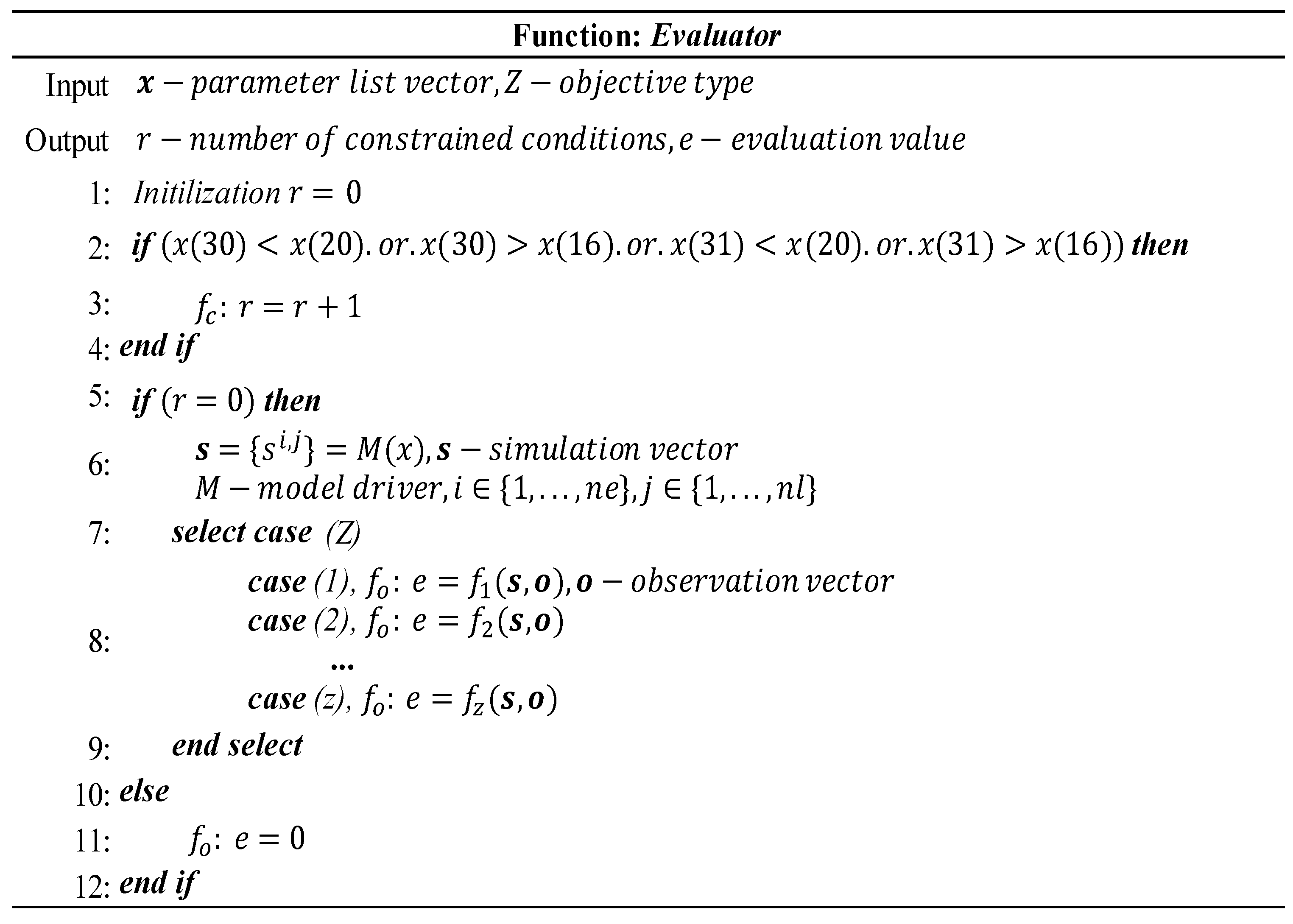
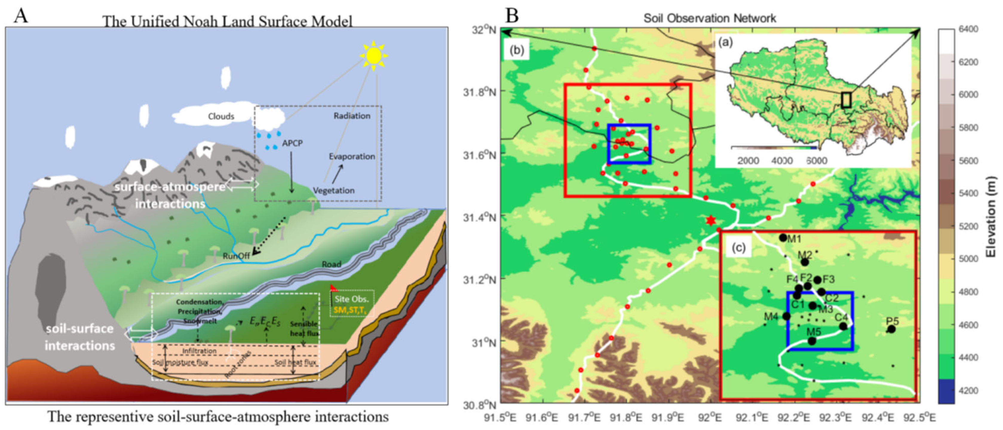
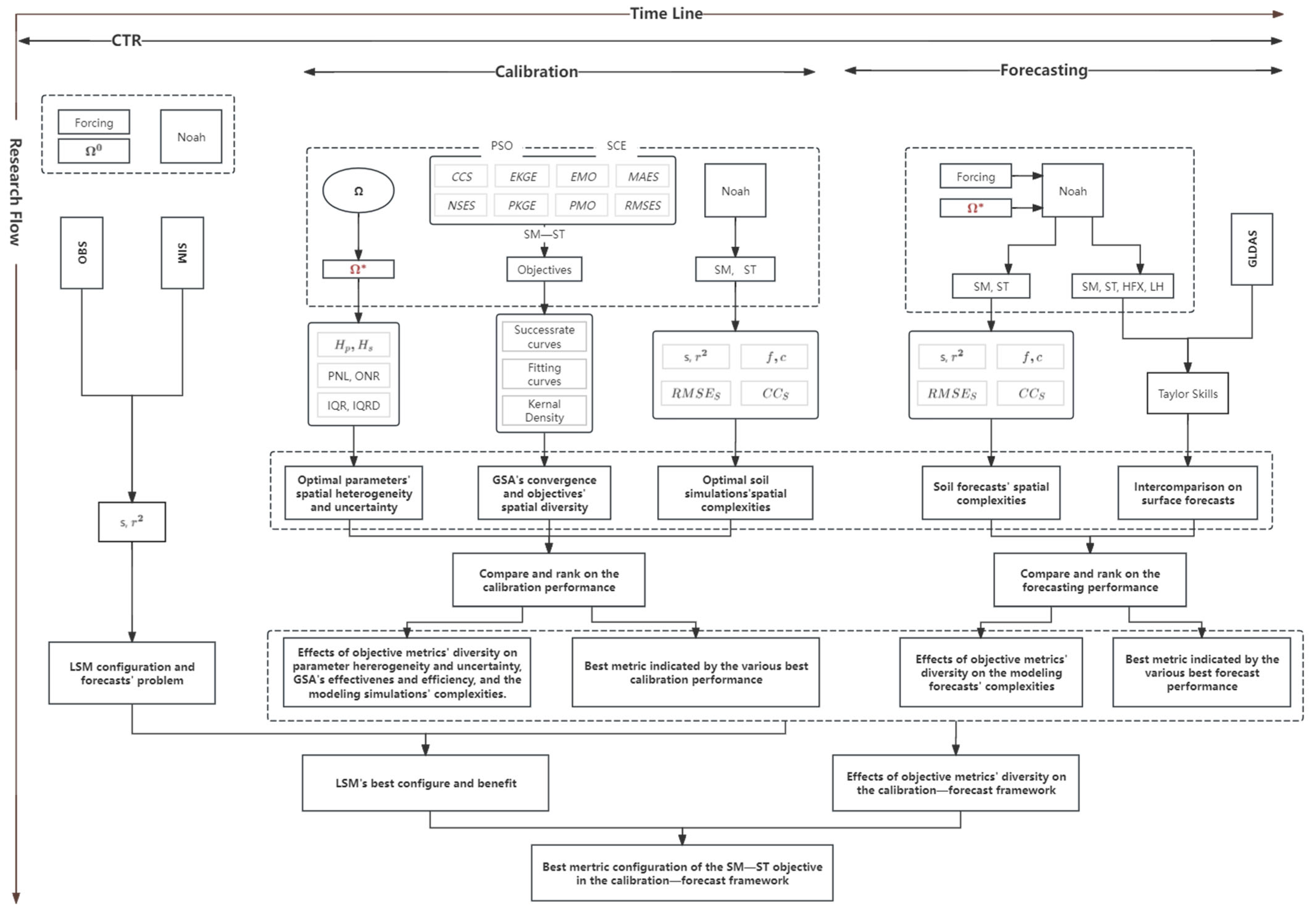
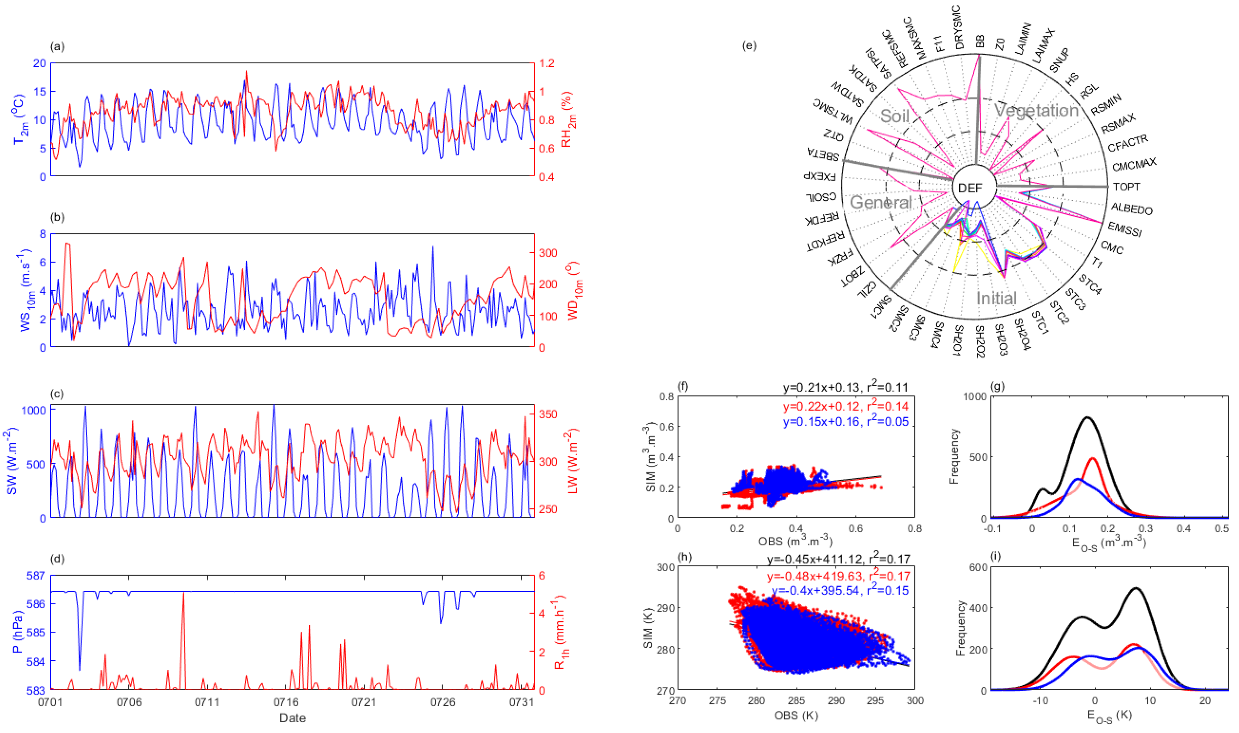

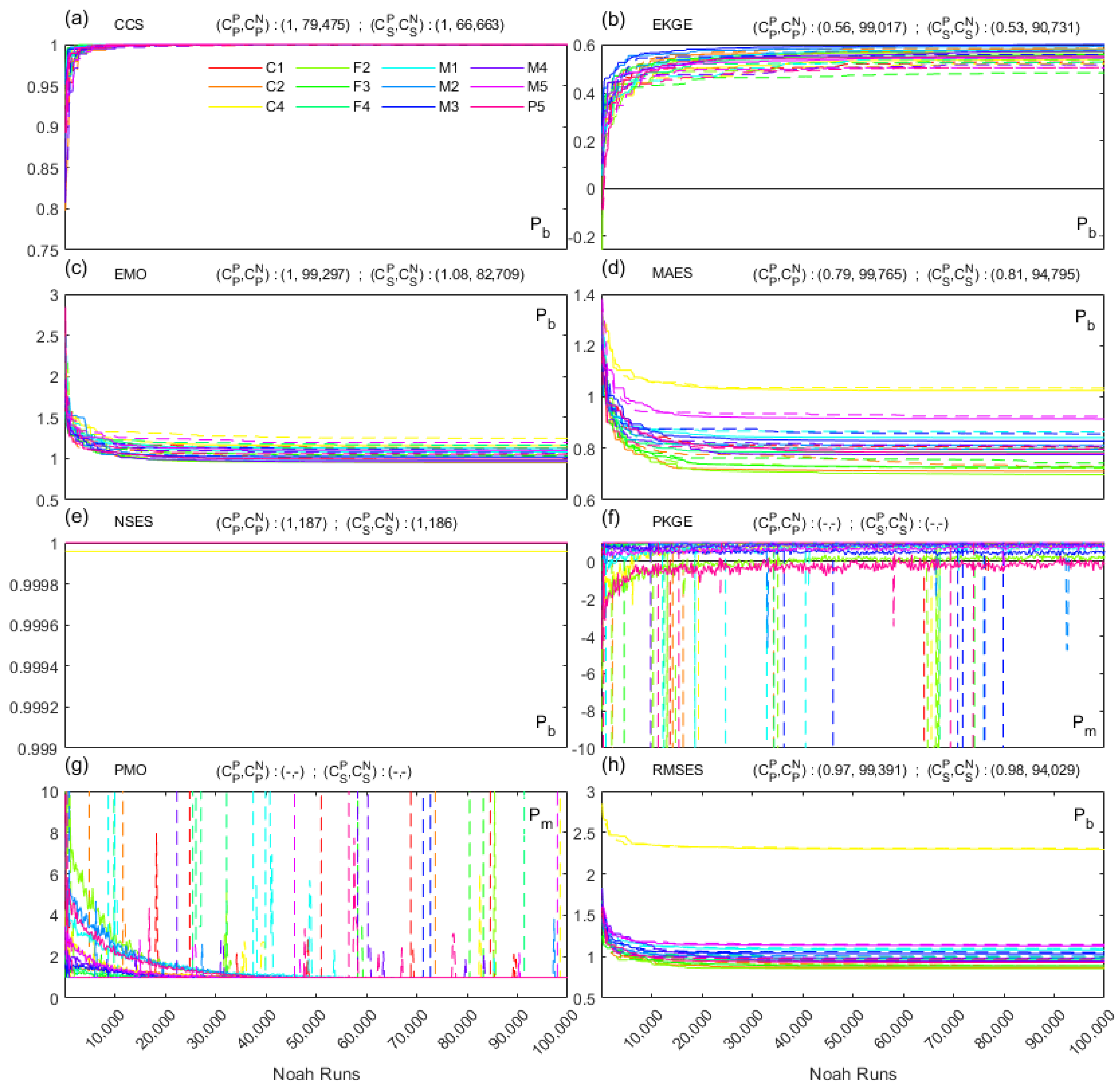
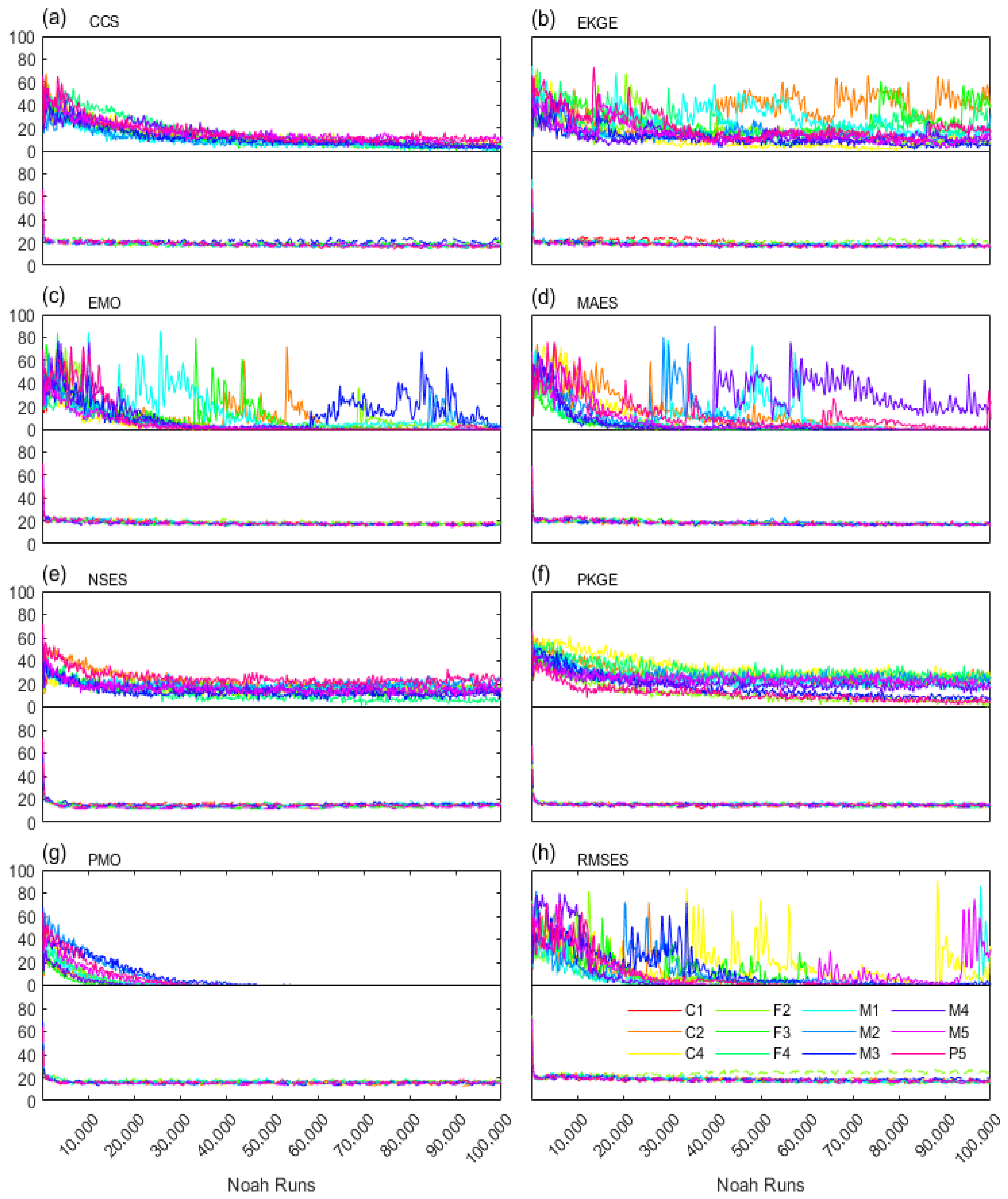
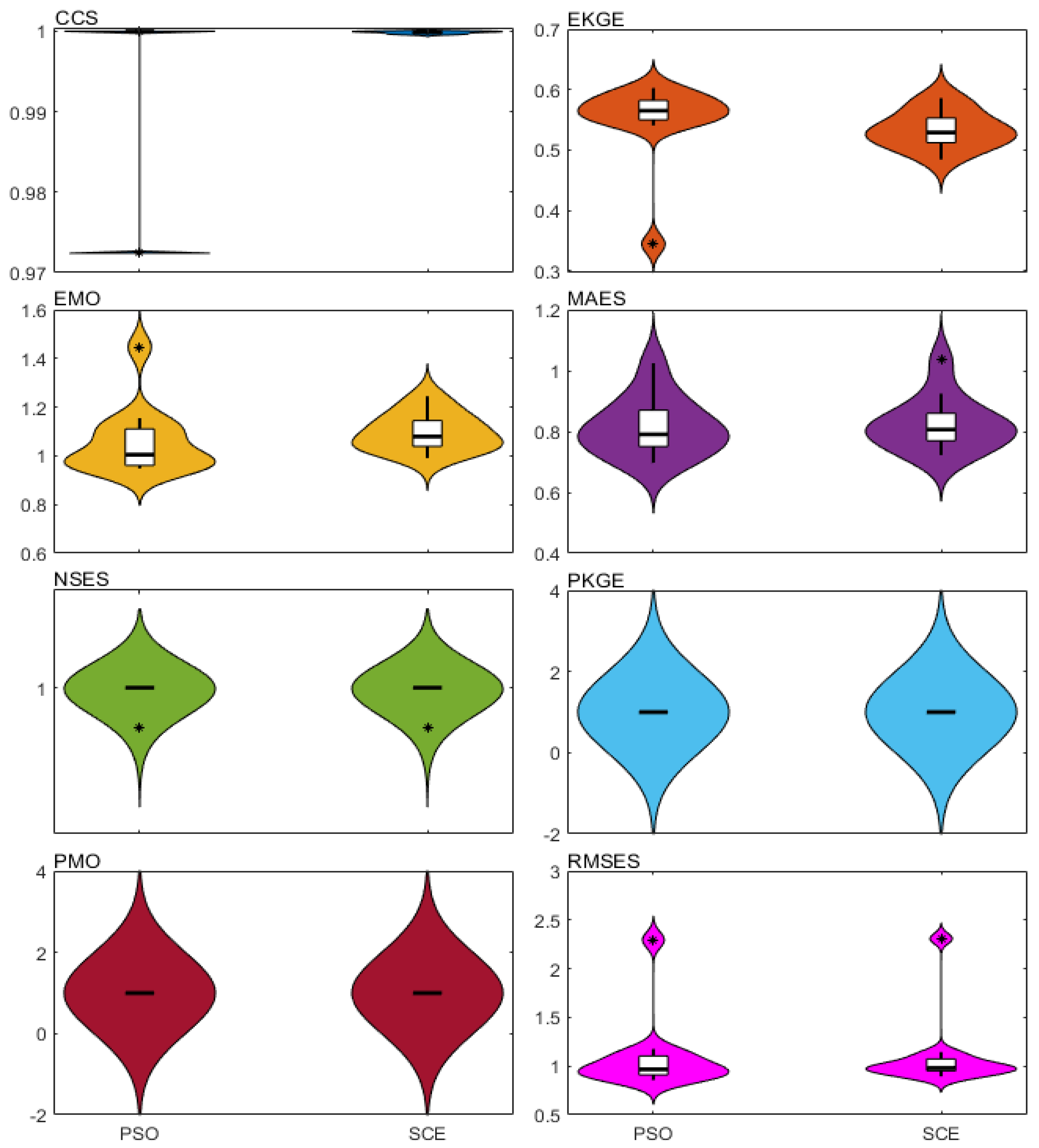
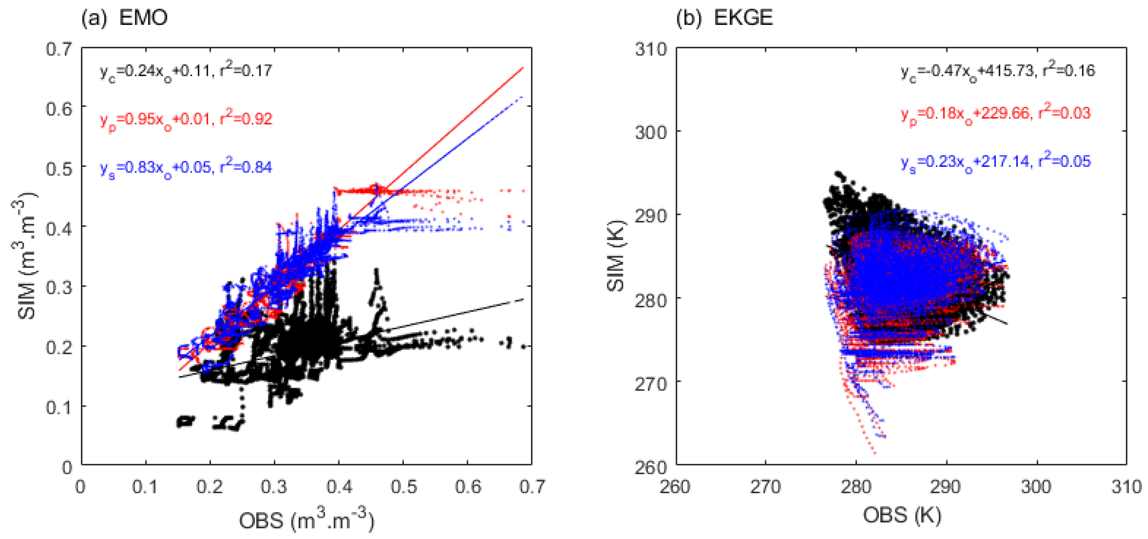
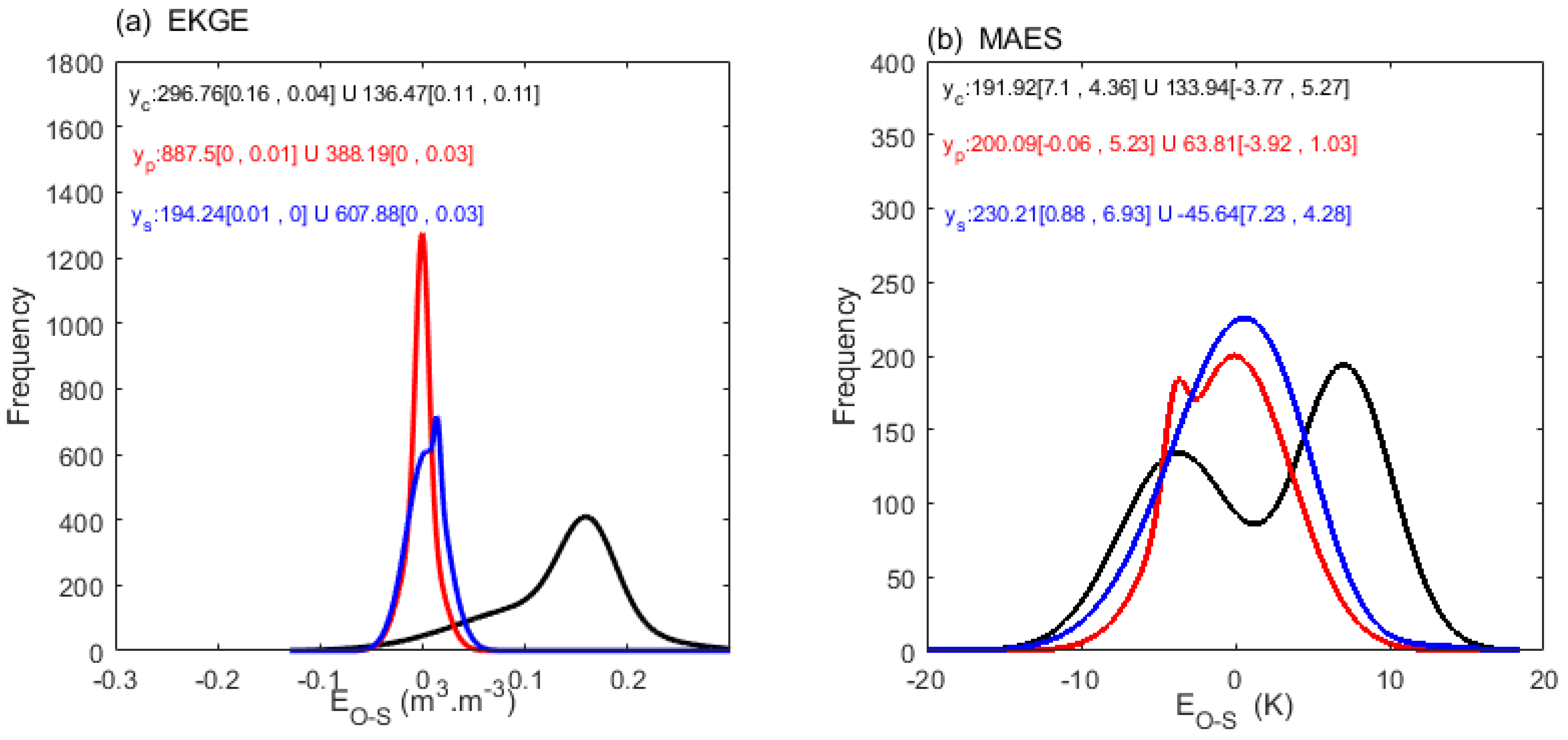
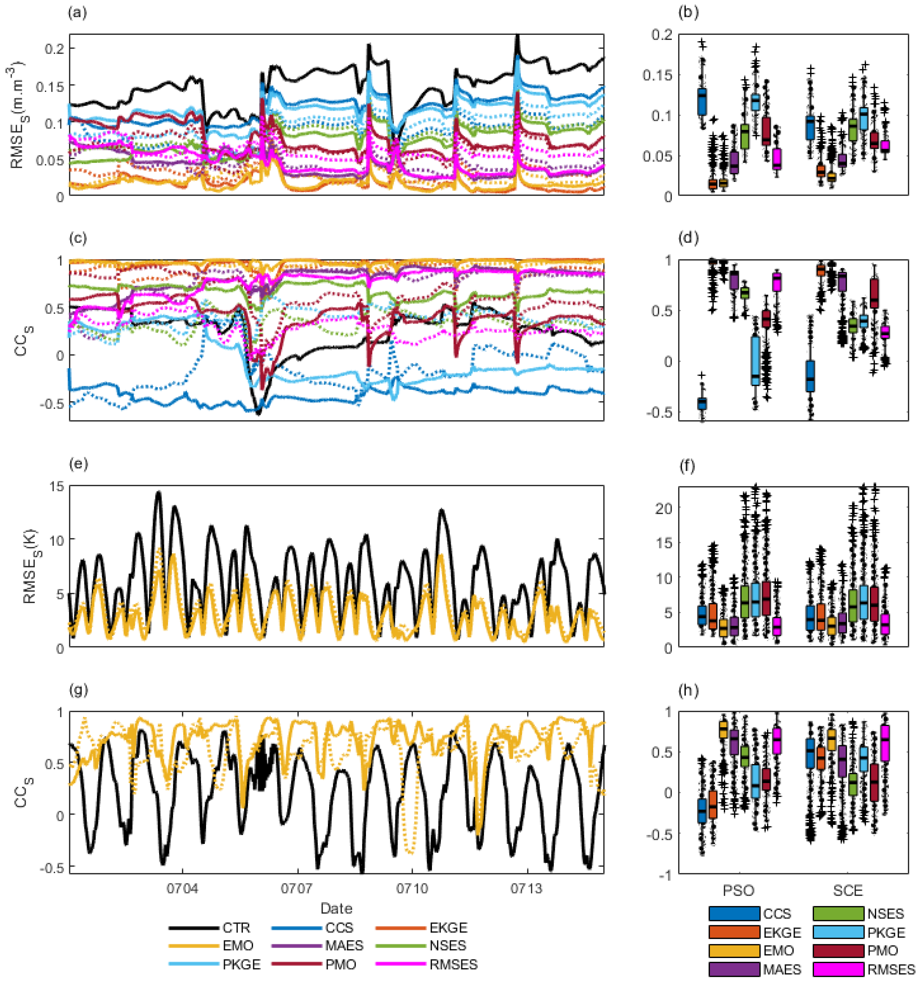

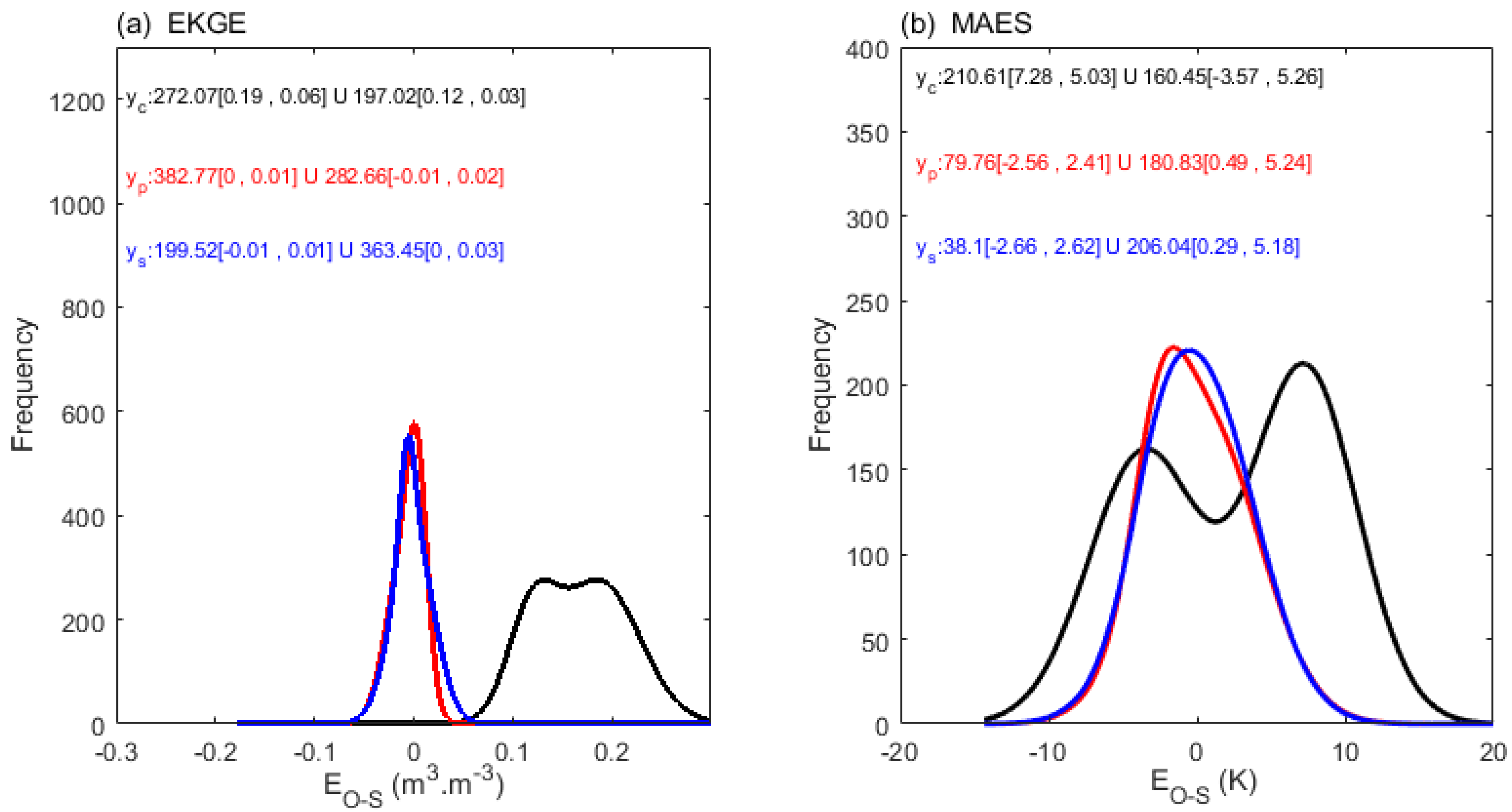
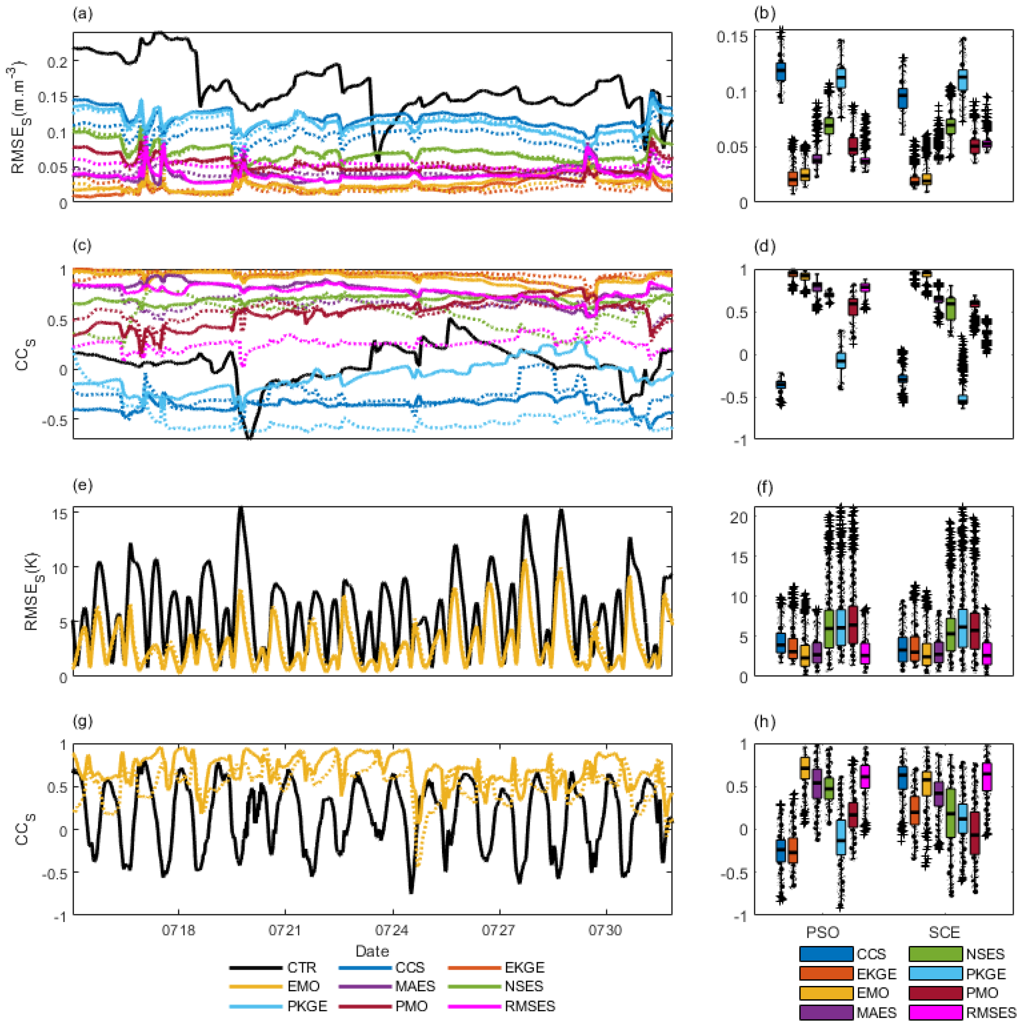
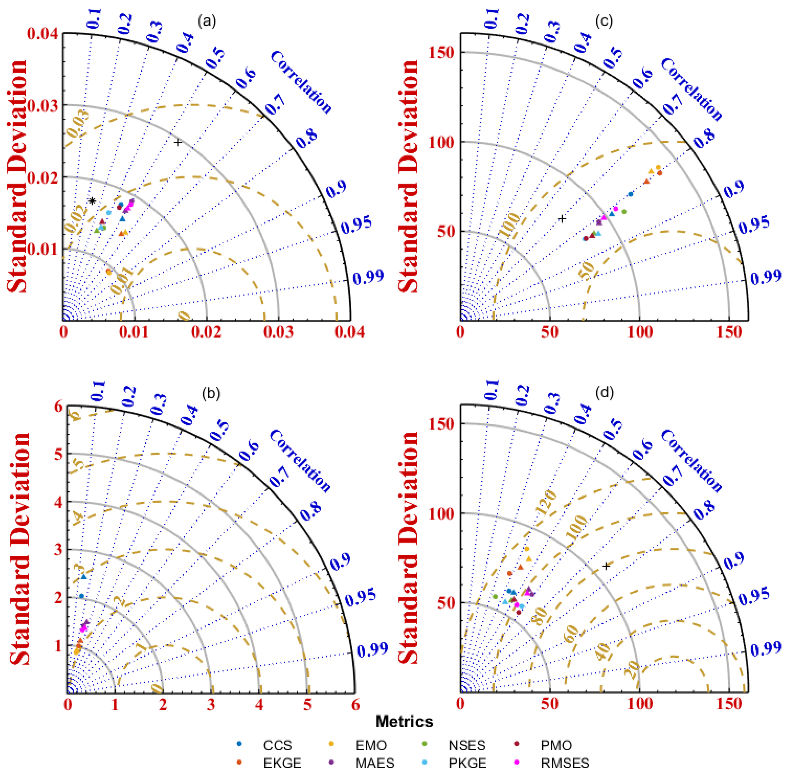
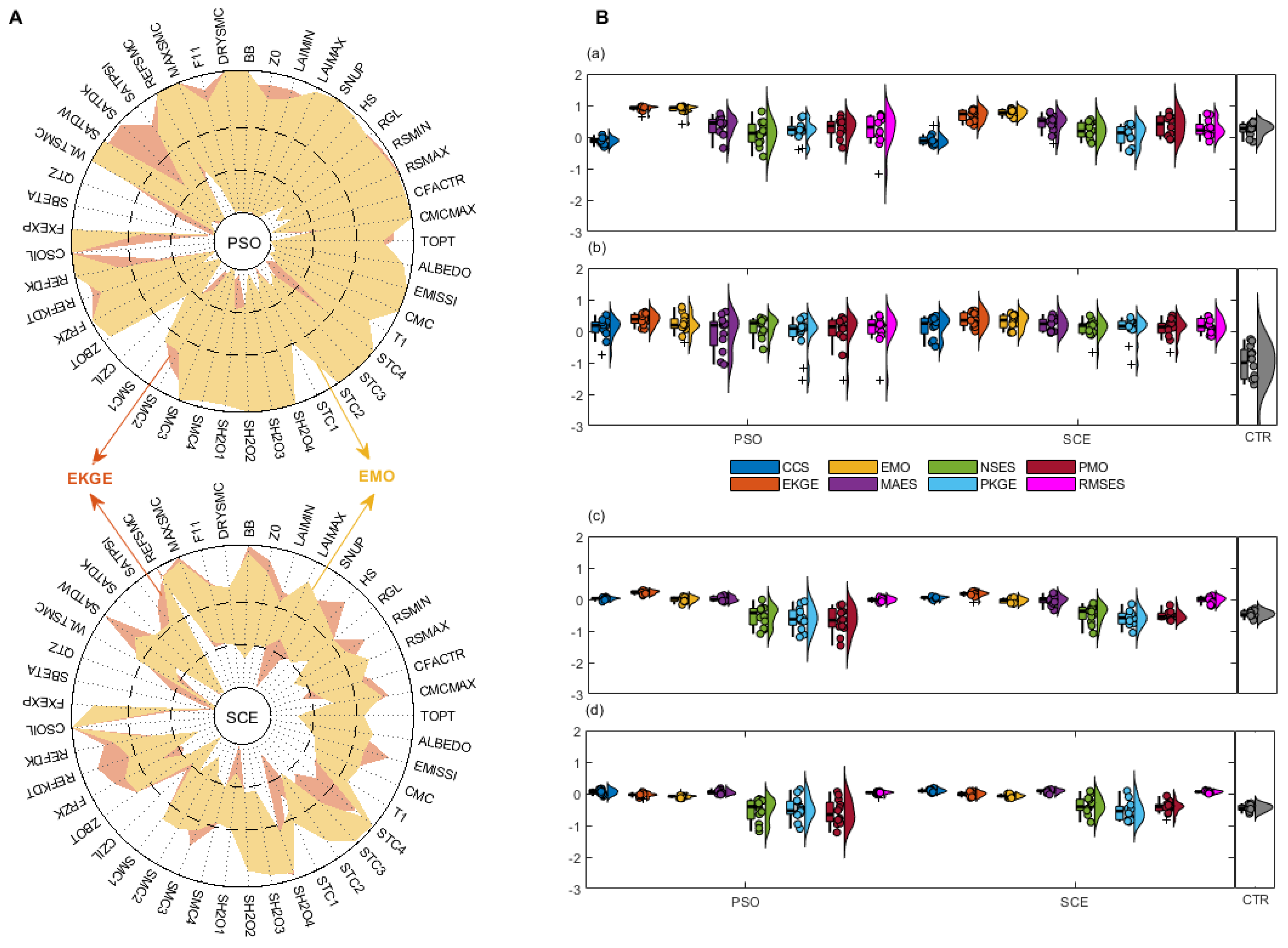
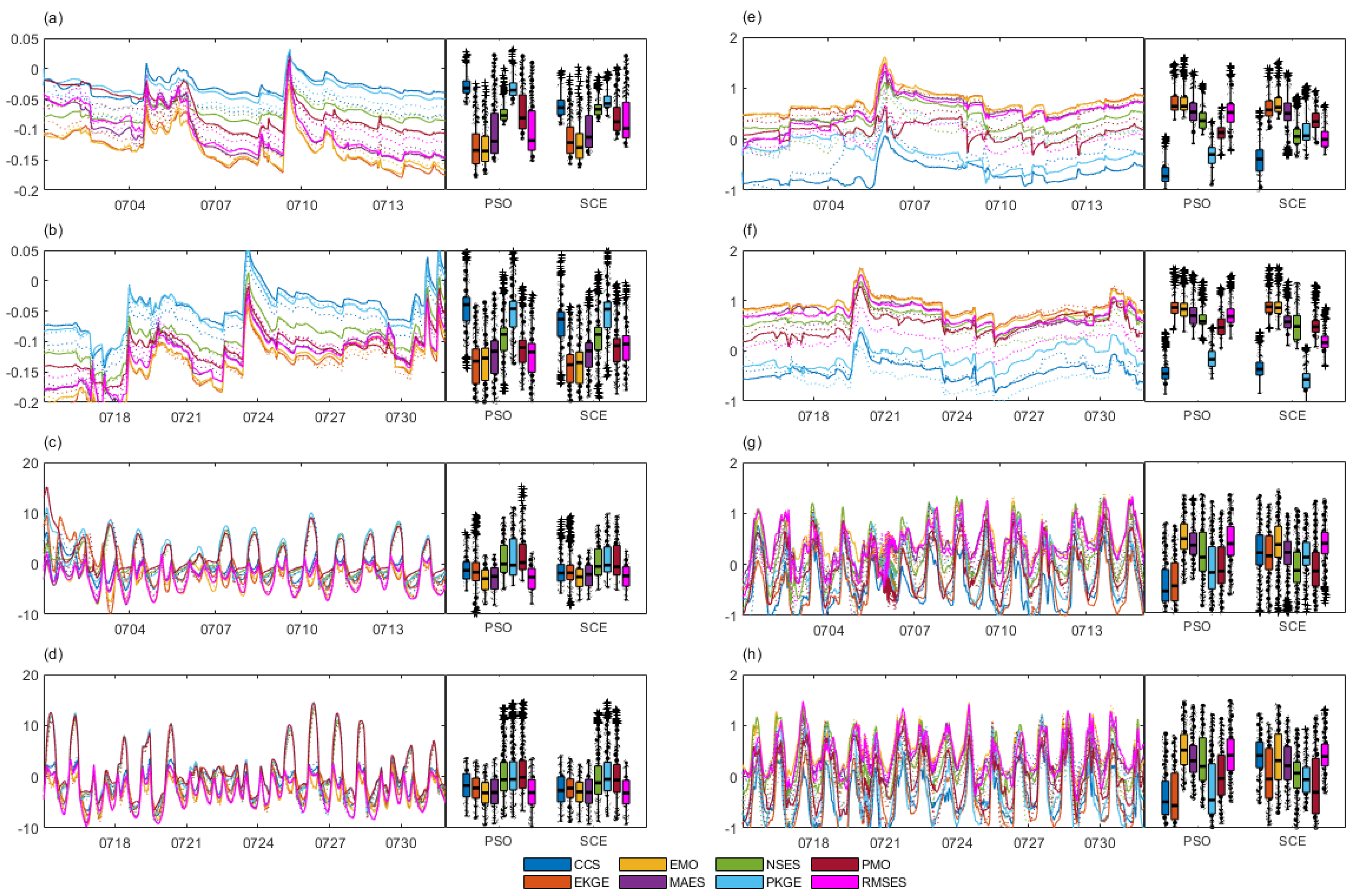
Disclaimer/Publisher’s Note: The statements, opinions and data contained in all publications are solely those of the individual author(s) and contributor(s) and not of MDPI and/or the editor(s). MDPI and/or the editor(s) disclaim responsibility for any injury to people or property resulting from any ideas, methods, instructions or products referred to in the content. |
© 2024 by the authors. Licensee MDPI, Basel, Switzerland. This article is an open access article distributed under the terms and conditions of the Creative Commons Attribution (CC BY) license (https://creativecommons.org/licenses/by/4.0/).