Abstract
With the increasing number of electric vehicles taking to the roads, the impact of tailpipe emissions on air quality will decrease, while resuspended road dust and brake/tire wear will become more significant. This study quantified PM10 emissions from tire wear under a range of real highway conditions with measurements across different seasons and roadway surface types in Phoenix, Arizona. Tire wear was quantified in the sampled PM10 using benzothiazoles (vulcanization accelerators) as tire markers. The measured emission factors had a range of 0.005–0.22 mg km−1 veh−1 and are consistent with an earlier experimental study conducted in Phoenix. However, these results are lower than values typically found in the literature and values calculated from emissions models, such as MOVES (MOtor Vehicle Emission Simulator). We found no significant difference in tire wear PM10 emission factors for different surface types (asphalt vs. diamond grind concrete) but saw a significant decrease in the winter compared to the summer.
1. Introduction
Vehicles are important sources of particulate matter (PM) emissions contributing to transportation-related air quality problems and greenhouse gases. Electrification of vehicle fleets for passenger and commercial uses is expected to increase exponentially in the next decade, which will drastically change the transportation sector’s emission profile [1]. With increasing fleet electrification, it is important to study how this change will affect vehicle emission profiles as tailpipe emissions decrease while non-exhaust emissions might increase due to heavier vehicles [2]. In regards to air quality impact, tailpipe PM emissions are primarily <2.5 μm (PM2.5) and consist of hydrocarbons, while non-exhaust emissions are usually <10 μm (PM10) and consist of heavy metals and microplastics from brake and tire wear [3,4]. Several studies have demonstrated that tire particle size is highly dependent on driving conditions, tire type, and pavement type, with a general trend of mechanical processes generating coarser particles and thermomechanical processes generating ultrafine particles [5,6,7]. In addition to an impact on PM air quality, tire particles can also leach out toxic chemicals into the environment, including benzothiazoles and N-(1,3-dimethylbutyl)-N′-phenyl-p-phenylenediamine (6PPD) [6,8,9]. However, in order to properly apportion PM10 emissions to tire-wear, a marker specific to tires must be used.
Wagner et al. (2018) [10] have detailed key criteria to consider when identifying a marker to be used in tire wear analysis. The marker should (1) be present in all tire materials in comparable portions largely independent from manufacturer/process, (2) not leach easily from tire particles into the surrounding environment, (3) not be easily transformed while the particles reside in the environment, (4) be sufficiently specific for tires, (5) have a concentration in tire material significantly higher than in particles forming the sample matrix, and (6) be analytically accessible by methods of high precision, accuracy, and sensitivity. An additional consideration is that the marker should remain constant regardless of the emission generation process/particle diameter.
While rubber is the main constituent of tires, it is a polymer of high molecular weight, making it difficult to study via chemical analyses; rather, one must use pyrolysis to generate rubber-specific volatile breakdown products, which then can be analyzed [10]. Styrene-butadiene rubber (SBR) is a common tire component used as a tire wear marker for air and soil samples where the pyrolysis products of styrene, butadiene, and vinylcyclohexene are the components being detected [11,12,13,14,15,16,17]. In addition to SBR, natural rubber, and butadiene rubber, zinc has been used as an elemental tracer for tire wear as it can make up for 1–2% of a tire’s mass [18,19,20].
Although vulcanization accelerators (benzothiazoles) only account for 0.5% of tire material, many studies have used these additives to quantify tire wear in the environment as a substantial amount of these compounds originate only from rubber, for example, Wik et al. (2009) [21]. The most commonly used benzothiazoles are 2-(4-morpholinyl)benzothiazole (24MoBT), originating from the 2-(Morpholinothio)benzothiazole (OBS) accelerator, and N-cyclohexyl-2-benzothizaolamine (NCBA), originating from the N-cyclohexyl-2-benzothiazole sulfenamide (CBS) accelerator [10]. Kim et al. (1990) [22] analyzed tire tread samples in addition to suspended PM and found that benzothiazole (BT) was common to all classes of tire tread tested and suitable for the quantitative determination of tire tread in suspended PM. Kumata et al. (1996) [23] developed a method for quantifying 24MoBT in environmental samples such as street dust, aerosols, and sediments. Building on this study, they were able to quantify 24MoBT and NCBA in street runoff, asphalt leach samples, and antifreeze samples [24]. Alexandrova et al. (2007) [25] also tested for the presence of 24MoBT and NCBA in aerosols, tire tread samples, and crumb rubber material (CRM). While they were able to quantify 24MoBT in the CRM and tire tread samples, they were unable to quantify 24MoBT or NCBA in their aerosol samples from a tunnel study. The biggest downside to using benzothiazoles as tire-wear markers is that the primary benzothiazoles used in rubber manufacturing are often transformed into other benzothiazole moieties during the rubber curing process. In addition, the organic extractions may require relatively harsh conditions or clean-up procedures, which are unideal [10].
Common methods for quantifying tire wear emissions include modeling, laboratory studies, and tunnel studies. It is primarily the emission factors generated from these studies that emission inventories use to apportion PM10 tire wear. For example, U.S. tire wear emissions are modeled using the U.S. EPA’s Motor Vehicle Emission Simulator Model (MOVES), which takes into account these types of studies [26]. MOVES has been used to model and estimate the emissions of carbon monoxide, nitrogen oxides, volatile organic compounds, and particulate matter, along with other pollutants coming from road vehicles like cars, trucks, and motorcycles and other non-road vehicles like tractors and agricultural equipment [27,28]. MOVES has been heavily used by a wide range of transportation stakeholders, including agencies, researchers, consultants, and policymakers, to make informed decisions that support emission reduction strategies on local, state, and regional levels.
In laboratory studies, a road simulator is used to generate tire wear, which can then be measured with instrumentation such as a DustTrak or scanning mobility particle sizer (SMPS) or sampled with impactors to be analyzed by transmission electron microscopy (TEM), scanning electron microscopy with energy-dispersive X-ray spectroscopy (SEM/EDX), or thermal–optical analysis [5,11,29,30,31,32]. These studies have been able to demonstrate a difference in PM10 generation from different types of tires (studded, non-studded, and summer) and road surfaces (granite and quartzite types of aggregates used on the surface) [5]. Aatmeeyata et al. (2009) [29] determined that small cars have a “large particle” non-exhaust emission factor ~6000 times higher than the non-exhaust PM10 emission factor. The benefit of this method is avoiding contamination from environmental sources and having direct control over a number of variables, including surface type, speed, and tire type; however, these types of studies are unable to properly simulate real driving conditions (swerving, hard braking, and accelerating) and environmental conditions. Additionally, if solely relying on a particle sizer, these studies may be unable to distinguish between tire wear and wear from the laboratory-simulated roadway surface.
Tunnel studies/receptor model studies have also been used to measure tire wear emissions but rely more heavily on source apportionment compared to laboratory studies. Typically, these studies conduct near-road sampling or tunnel exhaust sampling and use the aforementioned tire markers to conduct source apportionment or use principal component analysis to single out tire emissions [25,33,34,35,36]. Sjödin et al. (2010) [36] conducted both road simulator and field measurements and found reasonable agreement in total PM10 emission factors from both types of studies. Alexandrova et al. (2007) [25] conducted a tunnel study in Phoenix, AZ, and found a reduction in tire wear PM10 emissions with the use of an Asphalt Rubber Friction Course (AR) surface compared to existing Portland cement concrete (PCC) surfaces.
However, Wang et al. (2023) [34] demonstrated the difficulty of near-roadway sampling as their PM concentrations were heavily affected by wind direction and vehicle-induced turbulence. One approach used to alleviate this issue is the release of an artificial tracer. Historically, studies have released sulfur hexafluoride, an odorless, nontoxic, and relatively inert gas, at known rates to simulate pollutant releases [37,38]. By using the known tracer emission rate and the measured concentrations of tracer and pollutant of interest at the sampling point, the emission rate of the pollutant can be calculated. However, it is now known that sulfur hexafluoride is a potent greenhouse gas, and a gas tracer will not properly mimic specific sinks such as deposition when considering aerosol emissions. Cahill et al. (2016) [39] demonstrated the feasibility of using the ultrafine strontium (Sr) aerosol emissions from commercial road flares as an artificial aerosol tracer. All of these previous studies demonstrate challenges such as near roadway sampling difficulties, mixing of tire wear with other roadway emissions, and identifying appropriate tire markers that we seek to address in our present study.
The goal of this study was to quantify tire wear PM10 emissions and determine how different highway surfaces and seasons impact emission factors in real-world conditions. This was accomplished by deploying road flares onto highway surfaces to act as an artificial tracer line source for tire wear emissions, measured from a nearby overpass. Local tire samples were sourced and analyzed for tire markers (benzothiazoles) identified in the literature. This tire composition information was used to quantify tire wear PM10 in the highway samples. Sampling was conducted on the segments of highways with diamond-ground concrete surfaces (DG) and asphalt rubber friction course (AR) surfaces during the summer and winter. Using the tire marker and flare measurements and vehicle counts, tire wear PM10 emission factors were calculated for each sampling site. These emission factors were compared to estimated emission factors from running MOVES project-level models to assess model accuracy.
2. Experimental Materials and Methods
2.1. Sampling Site Selection
Sampling sites were chosen based on the presence of a low-traffic overpass or pedestrian bridge, traffic control concerns, and to ensure an even split between DG and AR surface types. Sites are listed in Table 1 and shown on a map in Figure 1. Samples taken at the SR 101L & E Sweetwater Ave, SR 101L & W Galveston St, and SR 101L & W Canal Path sites were obtained from the pedestrian bridges located at the listed cross-street. Sampling dates and times were restricted based on the requirements of the local department of transportation.

Table 1.
Sampling locations, surface type, and sampling date and time with winter samples marked with a W.
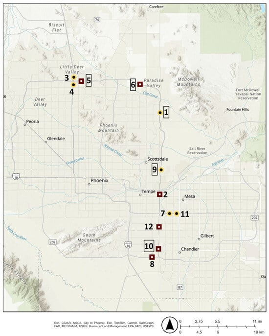
Figure 1.
Map of sampling sites with diamond-ground concrete surfaces (DG) sites in maroon and Asphalt Rubber Friction Course surfaces (AR) sites in gold. Whole numbers correspond to the sample numbers in Table 1, with numbers in boxes representing sites that winter samples were also collected at.
2.2. Sampling
2.2.1. Flare Testing
Preliminary flare testing was performed in a residential neighborhood with little through traffic. Flares were placed 2 m downwind of the Tisch PM10 high-volume air samplers (Tisch Environmental, Cleves, OH, USA), see Figure S1. Whatman Filter Paper 41 (cellulose) 8″ × 10″ and slotted filters (Cytiva, Marlborough, MA, USA) were used with a Tisch Series TE-235-Five Stage Cascade Impactor (Tisch Environmental, Cleves, OH, USA) to collect flare PM at several different size cuts, including <1.5 μm (PM1.5). Cellulose filters were used as received, but blanks were tested for Sr contamination. A residential Sr background, upwind flare, and downwind distant (45 m) flare were also tested at this location. Highway background samples for Sr and tire markers were also taken at the Maricopa County Air Quality Department’s (MCAQD) 33rd Ave near-roadway station, approximately 20 m south of I-10.
2.2.2. Highway Sample Collection
Highway PM10 samples for organics analysis were collected on pre-fired (overnight at 600 °C) Whatman 8″ × 10″ quartz microfiber filters using a Tisch PM10 high-volume air sampler pulling 1.1 m3/min. Highway PM1.5 samples for metals analysis were collected on cellulose filters (as received) using a Tisch PM10 high-volume air sampler with a Tisch Series TE-235-Five Stage Cascade Impactor attachment pulling 1.1 m3/min.
2.2.3. Highway Sampling Setup
Figure S2 demonstrates the sampling setup at a typical site where the sampling equipment was in the middle of the overpass while the flares were deployed in the high occupancy vehicle (HOV) lane, which was closed by traffic control. Even though the Sr emissions were from a small hot source being vertically entrained and the tire wear from multiple sources and influenced by vehicle wakes, we expect the two to be mixed by the time the emissions reach the samplers on the bridge. Since the flares only lasted ~30 min, to collect a one-hour sample, two flares were deployed at each of the 11 locations and lit sequentially; for two-hour samples, these were doubled to four flares at each location. Additionally on the overpass, temperature and relative humidity were recorded from a Control Company weather station, and the wind speed and direction were measured at a one-minute resolution using a WindLog Wind Data Logger (RainWise Inc., Boothwyn, PA, USA). For some sites, QuantAQ MODULAIR™-PM sensors (QuantAQ, Somerville, MA, USA) were used to collect PM1, PM2.5, and PM10 data and were placed on top of the overpass a few meters from the samplers. Finally, on the highway, a Commercial Electric (Cleveland, OH, USA) MS6520H infrared thermometer was used to measure the pavement surface temperature. Two one-hour samples were collected at 12 sites in the summer, with the original goal being to capture different traffic conditions just after rush hour (08:30–09:30) compared to a bit later (10:00–11:00). However, after initial traffic results were analyzed, there was little difference (∆4%) in traffic between these times, so we moved to one two-hour sample during the winter to maximize the amount of material collected onto the filters. Full traffic count data are shown in Table S1, while Figure S3 shows the light-duty vehicle (LDV) and heavy-duty vehicle (HDV) breakdown.
2.2.4. Tire Characterization
Sixteen used tire samples were obtained from CRM of America LLC in Queen Creek, Arizona, with a 50:50 split between LDV and HDV (Table S2). These samples were grinded with a Dremel power tool, and the resulting PM10 was collected on a pre-weighed, pre-baked 37 mm Whatman quartz filter with a low-volume air sampler using a PM10 Cyclone (URG Corporation, Chapel Hill, NC, USA) to achieve the size cut. Cyrogenic grinding was performed on a portion of the samples but did not produce sufficient PM10 material. A comparison test between cryogenically processed tire samples and Dremel processed tires confirmed that more tire markers were present in the Dremel samples and at higher concentrations.
2.3. Sample Preparation
After the highway and grinded tire samples on quartz fiber filters were returned to the laboratory, the highway quartz filters were weighed on a Denver Instrument APX-100 balance (with a modified balance pan to accommodate the filters) on three separate days in a glove box kept between 40 and 60% RH and a temperature of 21.5–24.5 °C, allowing 24 h for filters to equilibrate; the resuspended tire samples were only weighed once. If not immediately extracted, the filters were then placed in the freezer. Prior to extraction, the highway filters were cut into eighths, half of which were returned to their aluminum foil pouch and placed in the freezer, and the other half extracted. The resuspended tire samples were fully extracted. Moreover, 50 μL of the internal standard (Pyrene D10 and Benzo[α]pyrene D12) was dropped onto the filter sections and allowed to dry (previous tire studies, including Luhana et al., 2004 [40], have used these internal standards when analyzing benzothiazoles). The filter pieces were then cut into smaller pieces with an IPA-rinsed blade and placed sampled-side down into a beaker. The filters were then extracted three times with 30–40 mL of DCM (Fisher Scientific, Waltham, MA, USA, 99.9%) under sonication for 15 min. The combined extracts were evaporated under N2 to ~5 mL. The extract solution was filtered using a pre-baked Whatman quartz filter and evaporated further down to 100 μL and transferred to a GC-vial with a glass insert and kept in the freezer until analysis.
Cellulose filters from flare testing and highway sampling were kept in sealed plastic bags in the freezer prior to analysis. For 8″ × 10″ filters, analysis was performed in triplicate by using three 47 mm punches from the filters. For slotted filters, analysis was performed on one cut slot piece from the filter.
2.4. Sample Analysis
2.4.1. Chemicals and Materials
Primary tire marker standards used include 2-Hydrobenzothiazole (HOBT, Aldrich, St. Louis, MO, USA, 98%), 2-Phenylbenzothiazole (2PB, Sigma Aldrich, St. Louis, MO, USA, 97%), 2,2′-Dithiobis(benzothiazole) (MBTS, Aldrich, St. Louis, MO, USA, 99%), 2-(Methylthio)benzothiazole (MTBT, Aldrich, St. Louis, MO, USA, 97%), N-cyclohexyl-2-benzothiazole sulfenamide (CBS, AmBeed, Arlington Hts., IL, USA, 95%), N-cyclohexyl-1,3-benzothiazol-2-amine (NCBA, Enamide, 95%), Benzothiazole (BT, Aldrich, St. Louis, MO, USA, 97%), 2-Morpholin-4-yl-benzothiazole (24MoBT, Sigma Aldrich, St. Louis, MO, USA), 2-Methylbenzothiazole (MeBT, Aldrich, St. Louis, MO, USA, 99%), 2-Mercaptobenzothiazole (MBT, Aldrich, St. Louis, MO, USA, 97%), 4-(1,3-Dimethylbutylamino)diphenylamine (6PPD, Toronto Research Chemicals, Toronto, ON, Canada), and 6PPD-quinone (6PPDQ, HPC Standards, Atlanta, GA, USA, 95.64%). Internal standards included Pyrene D10 (Cambridge Isotope Laboratories Inc., Tewksbury, MA, USA, 98%) and Benzo[α]pyrene D12 (Cambridge Isotope Laboratories Inc., Tewksbury, MA, USA, 98%). Orion Safety Products 30 min flares with wire stand (Orion Safety Products, Easton, MD, USA) were used as the Sr emission source.
2.4.2. Organics Analysis
Chemical tire markers were quantified in the extracted highway and tire PM samples using Gas Chromatography Mass Spectrometry (GC-MS, Trace 1310 Gas Chromatograph, TSQ 9000 Triple Quadrupole Mass Spectrometer, TriPlus RSH Autosampler, Thermo Scientific, Waltham MA, USA). For tire samples, the injection volume was 1 μL, and for highway samples, it was 2.5 μL, with an injector temperature of 250 °C in splitless mode. A Thermo Scientific TG-5SILMS column was used (length of 30 m, diameter of 0.25 mm, and a film thickness of 0.25 μm). The oven was set to hold at 65 °C for the first 20 min, ramp to 200 °C at 10 °C/min and hold for 20 min, and then ramp to 275 °C at 10 °C/min and hold for 10 min, for a total runtime of 71 min. Helium was used as a carrier gas with a flow rate of 2.737 mL/min. The ion source was electron ionization, and the MS transfer line was at 250 °C and the ion source at 300 °C. The MS was in general acquisition mode, scanning masses 50–300 with a dwell time of 0.2 s. The quantification and confirmation ions and typical retention times for each tire marker are listed in Table S3, along with those with method detection limits.
2.4.3. Metals Analysis
Sr mass concentrations of highway samples were determined using Inductively Coupled Plasma-Mass Spectrometry (ICP-MS, NexION 2000, Perkin Elmer Inc., Waltham, MA, USA) after a microwave-assisted acid digestion. Filter samples were digested in a 20 mL Teflon vessel (Xpress, CEM Corporation, Charlotte, NC, USA) via microwave (Mars 5, CEM Corporation, Charlotte, NC, USA) using a digest solution composed of 10 mL nitric acid (HNO3 70%, Sigma Aldrich, MO, USA) + 4 mL H2O + 1 mL hydrofluoric acid (HF 40–60%, Sigma Aldrich, St. Louis, MO, USA). Following microwave digestion, the vessel contents were poured and evaporated at 160 °C in a 75 mL Teflon beaker until ~1 mL of solution remained. The evaporated solution was then diluted with 2% HNO3 in a 50 mL plastic volumetric flask and quantitatively transferred to a centrifuge tube for subsequent ICP-MS analysis. All sample preparation processes were carried out in the ULPA-filtered Class 10,000 cleanroom of the W. M. Keck Foundation Laboratory for Environmental Biogeochemistry at Arizona State University in a Class 10 vertical laminar flow/exhaust workstation to maintain sample cleanliness. Trace metal-grade acids (HNO3 and HF) and ultrapure water (18.2 MΩ, Milli-Q, Sigma Aldrich, Burlington, MA, USA) were used in the protocol to minimize reagent background. Prior to use, each container (Teflon vessel, Teflon beaker, plastic volumetric flask) was pre-cleaned with a 10% HNO3 soak overnight to prevent potential residual contamination. During ICP-MS analysis, an internal standard (10 ppb Sc, Ge, In, and Bi) was utilized to ensure a consistent sample injection rate during multielement ICP-MS analysis.
2.5. Emission Factor Calculation
Tire wear emission factors (EF) were calculated using Equation (1). The value of 0.1524 km arises from the length of the flare line source used at every sampling site (Figure S2), which was selected to ensure the flare emissions would be captured by the sampling device. This represents the effective distance of road that was sampled. The tire wear emission rate was calculated using Equation (2). The weighted average 2PB composition is further discussed in Section 3.2. The theoretical Sr mass emitted was calculated by multiplying the number of flares lit during the sample by the average Sr mass emitted by flares during testing (501,620 ng), as shown in Section 3.1. Uncertainty in the emission factor was calculated by propagating the errors in the marker, Sr, and flare emission measurements and is typical of previous studies quantifying aerosol markers using GC-MS [41,42].
2.6. MOVES Modeling
MOVES (MOVES 3.1, US EPA, Ann Arbor, MI, USA) utilizes a simple tire wear model to estimate tire wear emissions. Tire wear is calculated based on a simple regression model that incorporates vehicle speed as a single variable. After calculating the tire wear, the PM10 portion of the particulate matter is assumed to be eight percent of the total tire wear based on the findings of earlier studies [32,40]. Vehicle classification is accounted for by the number of tires each vehicle has. Vehicle speed and traffic counts are the primary factors that affect tire wear in MOVES simulations, as shown in Figure S4.
Project-scale analysis was conducted to obtain tire wear EFs for all sampled sites in order to compare the simulated tire wear emissions with the emissions derived from the field measurements. MOVES requires variable inputs to simulate tire wear emissions. Some inputs are required to calculate emissions, while others are necessary to calculate exhaust PM10 emissions, which are a prerequisite to running any tire wear emissions simulations. Some of these inputs and the sources of the used data are shown in Table S4. MOVES uses a slightly different vehicle classification system from that of the U.S. Federal Highway Administration (FHWA). The classes were interrelated for the purpose of this study, as shown in Table S5.
3. Results and Discussion
3.1. Flare Testing Results
Prior to field sampling, Sr measurements were made on flares to better characterize their emissions and to determine flare variability. Initial tests used an aluminum ductwork emission chamber to funnel flare emissions into the sampler; however, during operation, deposition of material to the ductwork was observed, suggesting that Sr was loss to the ductwork surface, so the chamber was not used during the rest of testing, see Figure S1. Out of 17 flares tested, the average runtime was 30.5 ± 1 min, with an average Sr emission rate of 269 ± 26 ng/s (502 ± 42 μg Sr emitted) and individual samples are shown in Table S6. Figure 2 shows the impact of the impactor size cut on the measured Sr concentration, with the smaller size cut (<1.5 μm) resulting in the highest concentration. This figure also shows that the residential and highway Sr backgrounds are lower than the flare test. The residential background is higher than the highway because it was performed after several flares had already been tested, and there was probably residual Sr still in the air, negating the usefulness of this sample. We also tested a flare ~45 m upwind of the samplers and still saw Sr concentrations 16 times higher than the highway background. Therefore, when using 22–44 flares per sample, we did not identify a need to develop a Sr background subtraction factor. An additional test of a blank cellulose filter confirmed that Sr values on a clean filter were ~2 orders of magnitude smaller than the residential Sr background.
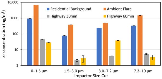
Figure 2.
Sr concentrations by impactor size cut from a residential background test, flare test, and two highway background tests by 33rd Ave and I-10.
Low-cost PM sensors were used to qualitatively confirm the transport of flare emissions from the highway to the overpass in real-time. While low-cost PM sensors may be subject to sampling bias, they provided real-time data to allow monitoring sampling progress. Figure 3 shows an example of this, as there are peaks in the PM1 and PM10 signals right when the flares were lit on the highway surface. Qualitatively, the peaks for the 2.1 sample are larger than sample 2.2; this is quantitatively represented in the Sr data, as sample 2.1 had 29% more Sr than sample 2.2. Additionally, when low Sr recovery (Sr on whole filter (ng)/Theoretical Sr Mass Emitted (ng)) was observed in the samples, the wind data often corroborated these results, showing that the wind direction during sampling was high or perpendicular to the flares and samplers.
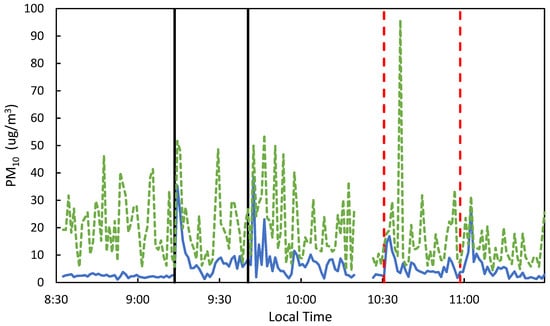
Figure 3.
PM1 (blue solid) and PM10 (green dashed) measurements from the MODULAIR™-PM sensor for samples 2.1 & 2.2. The black solid vertical lines represent lighting of flare sets for 2.1 and the red-dashed vertical lines for 2.2.
3.2. Tire Composition Results
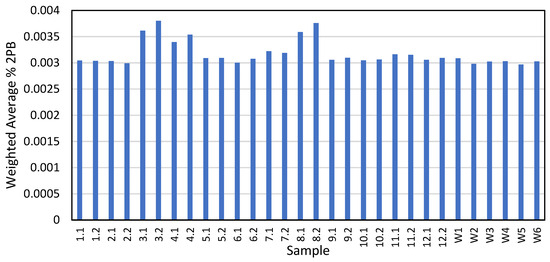
Several tire markers were identified and quantified in the 16 tire samples, summarized in Table 2. However, since 2PB was the only marker quantified in the majority of the highway samples, further calculations to convert from tire marker to tire wear only considered 2PB. First, the LDV 2PB composition was compared to the HDV 2PB composition, where HDV tires have a higher concentration of 2PB compared to LDV tires, an average of 0.0184% compared to 0.0027%. The composition of the traffic at each sampling location was examined. Figure S3 shows that LDV dominated the traffic composition. Therefore, a weighted 2PB composition average was developed for each sampling location, as shown in Figure 4, which was used to convert the mass of 2PB on the filter to the mass of tire wear.
Table 2.
Percent composition results for tire samples. Tire sample numbers correspond to Table S2.
3.3. Sampling Sites Environmental Results
Figure S5 summarizes the ambient temperature, surface temperature, and relative humidity values for all the samples. As expected, the summer samples have hotter temperatures and lower relative humidity than the winter samples. Additionally, for the summer samples, the samples taken later in the day are typically hotter and drier than the earlier samples. Figure S6 also shows the average wind speed during the sampling, where most samples had relatively calm wind except for 7.1, 7.2, 9.1, and 9.2 (no data were acquired for samples 2.1 & 2.2 due to wind sensor malfunction). With calmer wind conditions, we would expect a larger influence of transient winds generated by vehicles passing under the overpass on the dispersion characteristics of the tracer. In terms of wind direction, Table S7 shows the percentage of time for each sample that the wind direction is parallel with the flares and the PM samplers. Using this data, there was no clear correlation between calculated emission factor or Sr recovery and the wind direction. The average PM10 concentrations for each sample are shown in Figure 5. Data from sample 1.1 were omitted as it did not meet our quality standards while weighing, specifically the standard deviation for the triplicate measurements was more than 50% of the filter mass difference. Additionally, there was no difference in PM10 concentrations between AR and DG samples, and no clear correlation was observed between PM10 and vehicle counts for each sample. Other studies have also reported little correlation between vehicle counts and particle abundance, concluding that high levels of braking and acceleration are more influential variables [16,43].
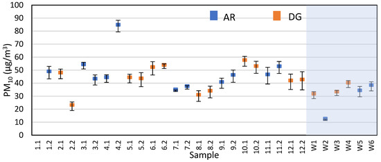
Figure 5.
Average PM10 concentrations with standard deviation from all samples as measured by gravimetry on the quartz fiber filters. The shaded box represents the winter samples.
3.4. Tire Wear Emission Factors for Different Highway Surfaces
Overall, 30 PM10 samples were collected by highways at a 50:50 split between AR and DG sites. Using Equation (1), the tire wear PM10 EF was calculated for each sample and shown in Table 3. Samples 1.1 & 1.2 were omitted due to anomalous mass measurements, samples 9.1 & 9.2 due to low Sr recovery values, and sample 10.1 due to an extraction error. Tire markers were not detected in samples W2–W6, so the EFs in Table 3 represent the maximum possible EF calculated from the 2PB method detection limit. In terms of sample–sample variability, higher EFs were observed at samples 2.1, 2.2, 4.1, 4.2, and 8.1 and 8.2. When inputting the same tire marker concentration (2PB Method Detection Limit (MDL) of 0.0286 μg/mL) into calculations for these samples, the same trend was observed (Figure S7). Using auxiliary data (Table S7), we determined that the higher EF values at 8.1 and 8.2 were due to low Sr recovery and the higher EFs at 2.1, 2.2, 4.1, and 4.2 were due to shorter sampling times than the rest of the samples. Therefore, these site-to-site differences are most likely more representative of the sensitivity of the method than any real differences between tire wear occurring between samples. This is also clear when comparing EFs for the different surfaces, as the averages and ranges are comparable: 6 × 10⁻² (1 × 10⁻²–2.2 × 10⁻¹) mg km−1 veh−1 for AR and 7 × 10⁻² (5 × 10⁻³–2.0 × 10⁻¹) mg km−1 veh−1 for DG. These EFs are an order of magnitude less than the values determined in most previous studies, such as Kupiainen et al. (2005) [32] (8.7 mg km−1 veh−1), Alves et al. (2020) [30] (2.0 mg km−1 veh−1), and Hicks et al. (2021) [44] (8.1 mg km−1 veh−1). However, Aatmeeyata et al. (2009) [29] calculated an EF of 3.7 × 10⁻³ mg km−1 veh−1, Ntziachristos and Boulter (2013) [45] found an EF range of 5–6 × 10⁻¹ mg km−1 veh−1, while a previous tunnel study in Phoenix, Arizona, calculated values of 1.2–3.5 × 10⁻¹ mg km−1 veh−1 [25].
Table 3.
Calculated tire wear emission factors for the summer and winter samples with uncertainty. Values calculated from method detection limits are shown in bold font.
3.5. Tire Wear Emission Factors for Different Seasons
Sampling was also reperformed at five of the sites (twice at one site) during the winter to determine whether environmental factors influence tire wear emission factors. Due to a number of factors, including site availability, construction, and a change in pavement surface, we were unable to revisit all 12 summer sites during the winter season. On average, the ambient temperature on winter sampling days was 29.1 °C cooler, the surface temperature was 37.8 °C cooler, and the relative humidity was 18.8% higher than the summer samples. Tire markers were not detected in five of the winter samples; therefore, the method detection limit of 2PB was used to calculate the potential maximum emission factor at those samples. It is apparent that winter tire wear emissions factors are much lower than the summer samples, with an average of 2 × 10⁻² and range of (5 × 10⁻³–3.0 × 10⁻²) mg km−1 veh−1 for winter compared to 8 × 10⁻² and (2 × 10⁻²–2.2 × 10⁻¹) mg km−1 veh−1 for summer. Additionally, the winter gravimetric PM10 was about 29% lower than the summer PM10. However, when looking at more short-term environmental changes, such as those between consecutive summer samples (higher temperatures and lower relative humidity for the second sample), no significant differences in EFs were observed.
Ejsmont et al. (2018) [46] demonstrated that tire rolling resistance is inversely proportional to air temperature. For example, a 30 °C decrease in air temperature resulted in a 28% increase in the coefficient of rolling resistance. This increased amount of friction is usually associated with increased tire wear; however, our results suggest that this tire wear may be larger than 10 μm, as we do not see an increase in PM10 tire wear in our winter samples compared to summer.
3.6. MOVES Simulated Emission Factors Comparison
After running the MOVES simulations, the output was normalized to obtain PM10 tire wear EFs for each location. The EFs for the summer sampling are shown in Figure 6A, while those for winter sampling are shown in Figure 6B. The calculated EFs for all samples were similar, with an average of 11.1 mg km−1 veh−1 across both sampling campaigns. This is expected as the vehicle speed is the major variable that affects tire wear emissions in MOVES. Vehicle speed on a highway was assumed to be constant in all simulations. Additionally, the traffic composition did not include any significant HDVs; therefore, it did not have any significant effect on the outcome of the simulations. The slight variation between the samples is minimal and within the expected range of error due to the relatively low precision in MOVES project level outputs. However, this variation follows the same pattern as the difference in traffic between the samples.
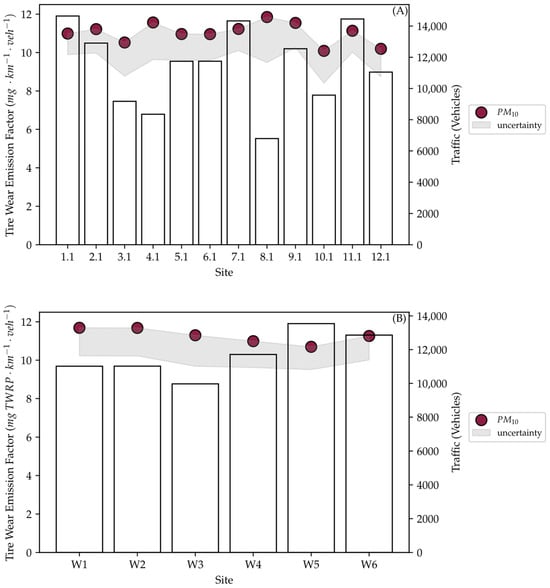
Figure 6.
MOVES simulated tire wear EFs for the summer samples (A) and winter samples (B).
The model simulations were not sensitive to the environmental effects, nor did the simulated EFs follow any particular trend when comparing summer and winter simulations, as they were only affected by traffic. The MOVES results were within range of values reported in the literature and were significantly higher than tire wear EFs measured during this field sampling campaign. Figure S8 presents the ratio of the simulated tire wear EFs to the ones calculated from field measurements. While MOVES may yield adequate estimates when applied on a national or county scale, caution is given on a project level. This is because factors such as seasonal effects (temperature, wind, and humidity changes) and surface type effects cannot be captured by MOVES [26].
MOVES3 establishes its tire wear PM10 emission factor calculation from Luhana et al., 2004 [40], where total tire wear loss rates were gravimetrically determined using LDVs, with an average of 74 mg km−1 veh−1 [26]. However, this study did not directly measure the PM10 emitted from tires and instead was limited to measuring a combined tire and brake wear emission factor of LDV’s in a tunnel of 6.9 mg km−1 veh−1. Furthermore, it appears that the EPA’s latest version of the model, MOVES4, does not include any updates to their PM10 tire wear emissions’ calculations, so these results should also be applicable to the newer model [47].
4. Conclusions
To better characterize tire wear PM10 emissions from highways, we conducted PM10 sampling at 12 different highway sites with varying pavement surfaces in a variety of environmental conditions. To account for mixing and transport between the highway surface and our sampling location, we used Sr-emitting road flares as an artificial PM tracer. Preliminary testing of these flares using a PM low-cost sensor and Sr measurements demonstrated the viability of this method to capture PM transport and mixing from the highway surface to our sampling locations. Additionally, tire markers, specifically benzothiazoles, were identified in the literature and later quantified in local tire samples. Both techniques were used in conjunction with traffic count data to calculate tire wear PM10 emission factors at the sample sites. A few of these EFs were of the same magnitude as a previous Phoenix, Arizona, tunnel study examining the same AR surface compared to a PCC surface. However, they were an order of magnitude lower than those in the most literature studies, emission inventories, and MOVES models.
One explanation for this discrepancy may be that the chosen chemical marker is not truly representative of the PM10 tire wear collected in this study, as minimal amounts of benzothiazole compounds were detected. However, these same compounds were detected when directly analyzing local tire samples. Calculations performed using the method detection limits of alternative markers such as NCBA and 6PPD yielded tire wear emission factors of the same magnitude as those calculated in this study using the 2PB marker. An alternative explanation may be that previous studies do not properly replicate the conditions experienced in Arizona at the time of our study. Additional concerns, such as the tire wear contribution of resuspended road dust, would lead to artificially inflated emission factors and would still not explain why the numbers in this study are lower than the most common literature values. Although the tire wear emission factors would be depressed if the flare testing setup did not adequately capture the emitted Sr, leading to an erroneously low flare Sr emission rate, this is not expected to be the case as the percent standard deviation of this measurement from multiple flares and days of testing was around 10%.
Even when site-specific conditions are accounted for in the MOVES model, such as in our study, the model still produced values an order of magnitude higher than the measured values as it was unable to simulate environmental conditions. This overestimation of project-level tire wear PM10 emissions by the MOVES model could mislead regulatory agencies in terms of enacting effective control measures for total PM10 emissions. Our results underscore the need for further tire wear emission factors studies and an eventual update of the MOVES prediction model to accurately capture tire wear-related PM10 emissions.
While there were some sample–sample differences in the calculated EFs, this can be explained by looking at supplemental data such as sampling time and Sr recovery. Additionally, even with two hours of sampling time, benzothiazole tire markers were unable to be detected in five of the winter samples. Perhaps using a more prevalent tire marker such as SBR or Zn could have made these measurements more quantitative. Regardless of the overall magnitude, when comparing EFs of AR and DG surfaces, no difference was observed. But when comparing winter to summer, EFs were significantly lower in the winter. This could be caused by a shift in the tire wear particle distribution to larger particles due to more brittle tires, which would not be captured by our PM10 samplers. While these particles would have less of an impact on air quality due to larger deposition velocities, they would still contribute to microplastic emissions in the environment. Overall, this study calls for more robust tire wear PM10 emission measurements in a variety of real-world conditions in order to more accurately quantify the impact of tire wear emissions on the environment.
Supplementary Materials
The following supporting information can be downloaded at: https://www.mdpi.com/article/10.3390/atmos15091122/s1, Figure S1: The initial aluminum ductwork emission chamber used to funnel flare emissions into the Tisch PM10 high-volume air sampler with the Tisch Series TE-235-Five Stage Cascade Impactor attachment (A). The final flare sampling configuration with the flare placed 2 m upwind of the sampler; Figure S2: Schematic of the sampling setup. Four flares were placed at each red marker, spaced 15.24 m apart. The figure is not to scale; Figure S3: LDV and HDV traffic composition for each sample; Table S1: Traffic counts for samples. Due to similarities in initial counts for sequential samples, traffic sampling was modified partway through the study to only conduct one hour of traffic count measurements. Samples with incomplete counts were extrapolated out to the full sampling period and are shown in bold; Table S2: Information about CRM of America LLC tire samples; Table S3: Quantification and confirmation ions for the tire markers and internal standards along with typical retention time (RT) and method detection limits (MDLs) if calculated; Figure S4: MOVES simulation for the generated amount of TW emissions with variable speed while fixing all other variables; Table S4: MOVES input data for project-level analysis; Table S5: MOVES classes counterparts in FHWA classification; Table S6: Results from flare testing Some samples are missing Sr masses as they were influenced by the aluminum ductwork, as shown in Figure S1, experienced analysis issues, or were a part of the distant flare testing; therefore, their data was only used in the average flare runtime calculation. Samples 14 and 15 and 16 and 17 were part of tests on multiple flares, and only one filter was collected; therefore, the mass represents emissions from two flares; Figure S5: Average ambient temperature (A), surface temperature (B), and relative humidity (C) values with maximum and minimum for all samples. The shaded box represents the winter samples; Figure S6: Average wind speed values with maximum and minimum for all samples; Table S7: Sr recovery values, sampling times, and percentage of time wind direction was parallel with the flares and samplers (+/−30°) for the samples; Figure S7: Tire wear EFs calculated using the 2PB method detection limit (0.0286 μg/mL); Figure S8: Ratio between simulated and measured tire wear emissions; Figure S9: Vehicle age distribution. Finally, the microwave digestion operational parameters are detailed.
Author Contributions
Conceptualization, M.P.F., P.H. and H.O.; methodology, M.P.F., P.H., J.A.M., S.A. and H.O.; formal analysis, J.A.M., Z.Z. and S.A.; investigation, J.A.M., Z.Z. and S.A.; resources, M.P.F., P.H. and H.O.; writing—original draft preparation, J.A.M. and S.A.; writing—review and editing, M.P.F., P.H., H.O., S.A. and J.A.M.; visualization, J.A.M. and S.A.; supervision, M.P.F., P.H. and H.O.; project administration, H.O.; funding acquisition, M.P.F., P.H. and H.O. All authors have read and agreed to the published version of the manuscript.
Funding
This study was funded by the Arizona Department of Transportation, Phoenix, AZ.
Institutional Review Board Statement
Not applicable.
Informed Consent Statement
Not applicable.
Data Availability Statement
The original contributions presented in the study are included in the article/Supplementary Materials, further inquiries can be directed to the corresponding author/s.
Acknowledgments
The authors would like to thank Kamil Kaloush, Jose Medina Campillo, Ramadan Salin, Grant Baumgardner, Parker Abel, Thuong Cao, Gabrielle Cano, Kanchana Chandrakanthan, Aidan McClure, Jesse Molar, Amelia Stout, Ashraf Alrajhi, Naagaviswanath Vedula, and Masih Beheshti for their support with this project’s field work and management.
Conflicts of Interest
The authors declare that they have no known competing financial interests or personal relationships that could have appeared to influence the study reported in this paper.
References
- Roca-Puigròs, M.; Marmy, C.; Wäger, P.; Beat Müller, D. Modeling the Transition toward a Zero Emission Car Fleet: Integrating Electrification, Shared Mobility, and Automation. Transp. Res. Part D Transp. Environ. 2023, 115, 103576. [Google Scholar] [CrossRef]
- Oroumiyeh, F.; Zhu, Y. Brake and Tire Particles Measured from On-Road Vehicles: Effects of Vehicle Mass and Braking Intensity. Atmos. Environ. X 2021, 12, 100121. [Google Scholar] [CrossRef]
- Pant, P.; Harrison, R.M. Estimation of the Contribution of Road Traffic Emissions to Particulate Matter Concentrations from Field Measurements: A Review. Atmos. Environ. 2013, 77, 78–97. [Google Scholar] [CrossRef]
- Piscitello, A.; Bianco, C.; Casasso, A.; Sethi, R. Non-Exhaust Traffic Emissions: Sources, Characterization, and Mitigation Measures. Sci. Total Environ. 2021, 766, 144440. [Google Scholar] [CrossRef]
- Gustafsson, M.; Blomqvist, G.; Gudmundsson, A.; Dahl, A.; Jonsson, P.; Swietlicki, E. Factors Influencing PM10 Emissions from Road Pavement Wear. Atmos. Environ. 2009, 43, 4699–4702. [Google Scholar] [CrossRef]
- Kole, P.J.; Löhr, A.J.; Van Belleghem, F.G.A.J.; Ragas, A.M.J. Wear and Tear of Tyres: A Stealthy Source of Microplastics in the Environment. Int. J. Environ. Res. Public Health 2017, 14, 1265. [Google Scholar] [CrossRef] [PubMed]
- Kreider, M.L.; Panko, J.M.; McAtee, B.L.; Sweet, L.I.; Finley, B.L. Physical and Chemical Characterization of Tire-Related Particles: Comparison of Particles Generated Using Different Methodologies. Sci. Total Environ. 2010, 408, 652–659. [Google Scholar] [CrossRef]
- Reddy, C.M.; Quinn, J.G. Environmental Chemistry of Benzothiazoles Derived from Rubber. Environ. Sci. Technol. 1997, 31, 2847–2853. [Google Scholar] [CrossRef]
- Tian, Z.; Zhao, H.; Peter, K.T.; Gonzalez, M.; Wetzel, J.; Wu, C.; Hu, X.; Prat, J.; Mudrock, E.; Hettinger, R.; et al. A Ubiquitous Tire Rubber–Derived Chemical Induces Acute Mortality in Coho Salmon. Science 2021, 371, 185–189. [Google Scholar] [CrossRef]
- Wagner, S.; Hüffer, T.; Klöckner, P.; Wehrhahn, M.; Hofmann, T.; Reemtsma, T. Tire Wear Particles in the Aquatic Environment—A Review on Generation, Analysis, Occurrence, Fate and Effects. Water Res. 2018, 139, 83–100. [Google Scholar] [CrossRef]
- Cadle, S.H.; Williams, R.L. Gas and Particle Emissions from Automobile Tires in Laboratory and Field Studies. J. Air Pollut. Control Assoc. 1978, 28, 502–507. [Google Scholar] [CrossRef]
- Lee, Y.-K.; Kim, M.G.; Whang, K.-J. Simultaneous Determination of Natural and Styrene-Butadiene Rubber Tire Tread Particles in Atmospheric Dusts by Pyrolysis-Gas Chromatography. J. Anal. Appl. Pyrolysis 1989, 16, 49–55. [Google Scholar] [CrossRef]
- Saito, T. Determination of Styrene-Butadiene and Isoprene Tire Tread Rubbers in Piled Particulate Matter. J. Anal. Appl. Pyrolysis 1989, 15, 227–235. [Google Scholar] [CrossRef]
- Unice, K.M.; Kreider, M.L.; Panko, J.M. Use of a Deuterated Internal Standard with Pyrolysis-GC/MS Dimeric Marker Analysis to Quantify Tire Tread Particles in the Environment. Int. J. Environ. Res. Public Health 2012, 9, 4033–4055. [Google Scholar] [CrossRef] [PubMed]
- Panko, J.M.; Chu, J.; Kreider, M.L.; Unice, K.M. Measurement of Airborne Concentrations of Tire and Road Wear Particles in Urban and Rural Areas of France, Japan, and the United States. Atmos. Environ. 2013, 72, 192–199. [Google Scholar] [CrossRef]
- Panko, J.M.; Hitchcock, K.M.; Fuller, G.W.; Green, D. Evaluation of Tire Wear Contribution to PM2.5 in Urban Environments. Atmosphere 2019, 10, 99. [Google Scholar] [CrossRef]
- Wei, P.; Sun, L.; Anand, A.; Zhang, Q.; Huixin, Z.; Deng, Z.; Wang, Y.; Ning, Z. Development and Evaluation of a Robust Temperature Sensitive Algorithm for Long Term NO2 Gas Sensor Network Data Correction. Atmos. Environ. 2020, 230, 117509. [Google Scholar] [CrossRef]
- Councell, T.B.; Duckenfield, K.U.; Landa, E.R.; Callender, E. Tire-Wear Particles as a Source of Zinc to the Environment. Environ. Sci. Technol. 2004, 38, 4206–4214. [Google Scholar] [CrossRef]
- Fauser, P.; Tjell, J.C.; Mosbaek, H.; Pilegaard, K. Quantification of Tire-Tread Particles Using Extractable Organic Zinc as Tracer. Rubber Chem. Technol. 1999, 72, 969–977. [Google Scholar] [CrossRef]
- Rhodes, E.P.; Ren, Z.; Mays, D.C. Zinc Leaching from Tire Crumb Rubber. Environ. Sci. Technol. 2012, 46, 12856–12863. [Google Scholar] [CrossRef]
- Wik, A.; Dave, G. Occurrence and Effects of Tire Wear Particles in the Environment—A Critical Review and an Initial Risk Assessment. Environ. Pollut. 2009, 157, 1–11. [Google Scholar] [CrossRef] [PubMed]
- Kim, M.G.; Yagawa, K.; Inoue, H.; Lee, Y.K.; Shirai, T. Measurement of Tire Tread in Urban Air by Pyrolysis-Gas Chromatography with Flame Photometric Detection. Atmos. Environ. Part A Gen. Top. 1990, 24, 1417–1422. [Google Scholar] [CrossRef]
- Kumata, H.; Takada, H.; Ogura, N. Determination of 2-(4-Morpholinyl)Benzothiazole in Environmental Samples by a Gas Chromatograph Equipped with a Flame Photometric Detector. Anal. Chem. 1996, 68, 1976–1981. [Google Scholar] [CrossRef]
- Kumata, H.; Yamada, J.; Masuda, K.; Takada, H.; Sato, Y.; Sakurai, T.; Fujiwara, K. Benzothiazolamines as Tire-Derived Molecular Markers: Sorptive Behavior in Street Runoff and Application to Source Apportioning. Environ. Sci. Technol. 2002, 36, 702–708. [Google Scholar] [CrossRef]
- Alexandrova, O.; Kaloush, K.E.; Allen, J.O. Impact of Asphalt Rubber Friction Course Overlays on Tire Wear Emissions and Air Quality Models for Phoenix, Arizona, Airshed. J. Transp. Res. Board 2007, 2011, 98–106. [Google Scholar] [CrossRef]
- U.S. Environmental Protection Agency. Brake and Tire Wear Emissions from Onroad Vehicles in MOVES3; Assessment and Standards Division, Office of Transportation and Air Quality, U.S. Environmental Protection Agency: Washington, DC, USA, 2020.
- Kota, S.H.; Zhang, H.; Chen, G.; Schade, G.W.; Ying, Q. Evaluation of On-Road Vehicle CO and NOx National Emission Inventories Using an Urban-Scale Source-Oriented Air Quality Model. Atmos. Environ. 2014, 85, 99–108. [Google Scholar] [CrossRef]
- Sentoff, K.M.; Aultman-Hall, L.; Holmén, B.A. Implications of Driving Style and Road Grade for Accurate Vehicle Activity Data and Emissions Estimates. Transp. Res. Part D Transp. Environ. 2015, 35, 175–188. [Google Scholar] [CrossRef]
- Aatmeeyata; Kaul, D.S.; Sharma, M. Traffic Generated Non-Exhaust Particulate Emissions from Concrete Pavement: A Mass and Particle Size Study for Two-Wheelers and Small Cars. Atmos. Environ. 2009, 43, 5691–5697. [Google Scholar] [CrossRef]
- Alves, C.A.; Vicente, A.M.P.; Calvo, A.I.; Baumgardner, D.; Amato, F.; Querol, X.; Pio, C.; Gustafsson, M. Physical and Chemical Properties of Non-Exhaust Particles Generated from Wear between Pavements and Tyres. Atmos. Environ. 2020, 224, 117252. [Google Scholar] [CrossRef]
- Dahl, A.; Gharibi, A.; Swietlicki, E.; Gudmundsson, A.; Bohgard, M.; Ljungman, A.; Blomqvist, G.; Gustafsson, M. Traffic-Generated Emissions of Ultrafine Particles from Pavement–Tire Interface. Atmos. Environ. 2006, 40, 1314–1323. [Google Scholar] [CrossRef]
- Kupiainen, K.J.; Tervahattu, H.; Räisänen, M.; Mäkelä, T.; Aurela, M.; Hillamo, R. Size and Composition of Airborne Particles from Pavement Wear, Tires, and Traction Sanding. Environ. Sci. Technol. 2005, 39, 699–706. [Google Scholar] [CrossRef] [PubMed]
- Amato, F.; Alastuey, A.; de la Rosa, J.; Gonzalez Castanedo, Y.; Sánchez de la Campa, A.M.; Pandolfi, M.; Lozano, A.; Contreras González, J.; Querol, X. Trends of Road Dust Emissions Contributions on Ambient Air Particulate Levels at Rural, Urban and Industrial Sites in Southern Spain. Atmos. Chem. Phys. 2014, 14, 3533–3544. [Google Scholar] [CrossRef]
- Wang, X.; Gronstal, S.; Lopez, B.; Jung, H.; Chen, L.-W.A.; Wu, G.; Ho, S.S.H.; Chow, J.C.; Watson, J.G.; Yao, Q.; et al. Evidence of Non-Tailpipe Emission Contributions to PM2.5 and PM10 near Southern California Highways. Environ. Pollut. 2023, 317, 120691. [Google Scholar] [CrossRef] [PubMed]
- Weckwerth, G. Verification of Traffic Emitted Aerosol Components in the Ambient Air of Cologne (Germany). Atmos. Environ. 2001, 35, 5525–5536. [Google Scholar] [CrossRef]
- Sjödin, Å.; Ferm, M.; Björk, A.; Rahmberg, M.; Gudmundsson, A.; Swietlicki, E.; Johansson, C.; Gustafsson, M.; Blomqvist, G. Wear Particles from Road Traffic—A Field, Laboratory and Modelling Study. Final Report; IVL Swedish Environmental Research Institute: Göteborg, Sweden, 2010. [Google Scholar]
- Dietz, R.N.; Cote, E.A. Tracing Atmospheric Pollutants by Gas Chromatographic Determination of Sulfur Hexafluoride. Environ. Sci. Technol. 1973, 7, 338–342. [Google Scholar] [CrossRef]
- Whiteman, C.D.; Glover, D.W. Technique for Elevated Release of Sulfur Hexafluoride Tracer. J. Air Pollut. Control Assoc. 1983, 33, 772–774. [Google Scholar] [CrossRef]
- Cahill, T.A.; Barnes, D.E.; Wuest, L.; Gribble, D.; Buscho, D.; Miller, R.S.; De la Croix, C. Artificial Ultra-Fine Aerosol Tracers for Highway Transect Studies. Atmos. Environ. 2016, 136, 31–42. [Google Scholar] [CrossRef][Green Version]
- Luhana, L.; Sokhi, R.; Warner, L.; Mao, H.; Boulter, P.; McCrae, I.; Wright, J.; Osborn, D. Non-Exhaust Particulate Measurements: Results. In Deliverable 8 of the European Commission DG TrEn, 5th Framework PARTICULATES Project, Contract No. 2000-RD.11091; European Commissions, Directorate General Transport and Environment: Brussel, Belgium, 2004; p. 96. [Google Scholar]
- Mazurek, M.A.; Simoneit, B.R.T.; Cass, G.R.; Gray, H.A. Quantitative High-Resolution Gas Chromatography and High-Resolution Gas Chromatography/Mass Spectrometry Analyses of Carbonaceous Fine Aerosol Particles. Int. J. Environ. Anal. Chem. 1987, 29, 119–139. [Google Scholar] [CrossRef]
- Rogge, W.F.; Mazurek, M.A.; Hildemann, L.M.; Cass, G.R.; Simoneit, B.R.T. Quantification of Urban Organic Aerosols at a Molecular Level: Identification, Abundance and Seasonal Variation. Atmos. Environ. Part A Gen. Top. 1993, 27, 1309–1330. [Google Scholar] [CrossRef]
- Knight, L.J.; Parker-Jurd, F.N.F.; Al-Sid-Cheikh, M.; Thompson, R.C. Tyre Wear Particles: An Abundant yet Widely Unreported Microplastic? Environ. Sci. Pollut. Res. Int. 2020, 27, 18345–18354. [Google Scholar] [CrossRef]
- Hicks, W.; Beevers, S.; Tremper, A.H.; Stewart, G.; Priestman, M.; Kelly, F.J.; Lanoisellé, M.; Lowry, D.; Green, D.C. Quantification of Non-Exhaust Particulate Matter Traffic Emissions and the Impact of COVID-19 Lockdown at London Marylebone Road. Atmosphere 2021, 12, 190. [Google Scholar] [CrossRef]
- Ntziachristos, L.; Boulter, P. Road Vehicle Tyre and Brake Wear. In EMEP/EEA Emission Inventory Guidebook 2013; European Environment Agency: Copenhagen, Denmark, 2013. [Google Scholar]
- Ejsmont, J.; Taryma, S.; Ronowski, G.; Swieczko-Zurek, B. Influence of Temperature on the Tyre Rolling Resistance. Int. J. Automot. Technol. 2018, 19, 45–54. [Google Scholar] [CrossRef]
- U.S. Environmental Protection Agency. Overview of EPA’s MOtor Vehicle Emission Simulator (MOVES4); Assessment and Standards Division, Office of Transportation and Air Quality, U.S. Environmental Protection Agency: Washington, DC, USA, 2023.


Disclaimer/Publisher’s Note: The statements, opinions and data contained in all publications are solely those of the individual author(s) and contributor(s) and not of MDPI and/or the editor(s). MDPI and/or the editor(s) disclaim responsibility for any injury to people or property resulting from any ideas, methods, instructions or products referred to in the content. |
© 2024 by the authors. Licensee MDPI, Basel, Switzerland. This article is an open access article distributed under the terms and conditions of the Creative Commons Attribution (CC BY) license (https://creativecommons.org/licenses/by/4.0/).