Abstract
Elevated O3 concentrations pose a significant threat to human health and ecosystems, but little research has been performed on coastal wetlands near large cities. This study focuses on investigating the key factors affecting O3 formation in the ecologically sensitive Dongtan Wetland (Chongming District, Shanghai, China) area. By comparing the performance of O3 concentration prediction of multiple machine learning models, this study found that the random forest model achieved the highest accuracy (R2 = 0.9, RMSE = 11.5). Feature importance and structure mining showed that peroxyacetyl nitrate (PAN), nitrogen oxides (NOx), temperature, wind direction, and relative humidity were the main drivers of O3 formation. Specifically, PAN concentrations exceeding 0.1 ppb and temperatures above 3 °C were found to have a significant impact on O3 levels, especially in spring, summer, and autumn. Trajectory analysis showed that westward urban pollution and emissions transported from the ocean were the main factors in O3 formation in the area. This study highlights the need for targeted emission control strategies, especially for PAN precursors generated by ships and NOx generated by urban industries, providing important insights for improving air quality in ecologically sensitive coastal areas.
1. Introduction
Ozone (O3) pollution has become an environmental issues of global concern [1]. O3 is not only a greenhouse gas but also has a significant impact on surface air quality and human health [2]. Since 2013, China’s fine particulate matter (PM2.5) concentration has dropped by 30–40%, but since the implementation of the “Air Pollution Prevention and Control Action Plan” in 2013, the ambient O3 concentration in many Chinese cities has remained high [3]. The 90th percentile of the maximum 8 h average daily O3 in Shanghai in 2023 is 158 μg/m3, which has not changed much from 163 μg/m3 in 2013 [4]. Therefore, O3 pollution has become a growing concern in Shanghai and across China. Although the fundamental mechanisms of O3 formation are well understood, the region-specific drivers of O3 generation need further study to develop targeted control strategies.
The formation of O3 involves many drivers, including precursor substances, chemical processes, and meteorological conditions [5]. Nitrogen oxides (NOx) and volatile organic compounds (VOCs) are the main precursors of O3. They are generated through complex chemical reactions under the action of sunlight [6,7]. Meteorological conditions such as temperature, humidity, wind speed, and solar radiation significantly affect the generation and distribution of O3. High temperatures and strong ultraviolet radiation usually promote the formation of O3. Drought-induced decreases in relative humidity can trigger stomatal closure in forest ecosystems, reducing stomatal O3 flux and weakening the ecosystem’s O3 removal capacity, which may contribute to elevated ambient O3 concentrations [8]. The generation mechanism of O3 may vary in different regions, depending on local pollutant emissions, meteorological conditions, and geographical characteristics [9]. Secondary organic carbon (SOC) and primary organic carbon (POC) in the atmosphere also influence O3 concentrations. In the machine learning-based driver analysis, SOC contributed approximately 8% to O3 prediction, while POC accounted for about 4%, indicating their non-negligible roles in O3 formation [10]. In addition, PAN, as an important secondary pollutant, plays a key role in the formation of O3 [11]. PAN is primarily generated by the reaction of peroxyacetyl radicals with nitrogen dioxide, which are formed by the oxidation of various VOCs and oxygenated VOCs (OVOCs) [12]. PAN can act as a reservoir for NOx, affecting the generation of long-range O3 [13]. PAN is known to be 1–2 orders of magnitude more biologically toxic than O3 [14]. Numerous studies have found that, compared to urban areas, high concentrations of PAN are primarily observed in suburban regions [11,15,16]. Given its known biological toxicity to humans, it is crucial to incorporate PAN into the analysis of O3 formation mechanisms in these areas. Additionally, attention should be paid to the interaction between PAN and O3, as well as their combined impact on air quality and human health.
Conventional approaches to studying O3 pollution rely primarily on deterministic physical and chemical models, which require extensive computing resources and precise input data and often have difficulty capturing complex nonlinear relationships [17,18,19]. Machine learning technology has significant advantages in handling large-scale data and complex nonlinear relationships [20]. With the development of machine learning technology, interpretable machine learning models have gradually gained attention. These models can not only provide high-precision predictions but also reveal the logic behind model decisions and feature importance, which helps to understand the O3 generation mechanism. In order to comprehensively analyze the impact of different factors on O3 concentration, in recent years, various ML methods, such as random forest (RF) [21], recurrent neural networks (RNNs) [22], and artificial neural networks (ANNs) [23], have been applied to predict the concentrations of atmospheric pollutants (O3, PM2.5, NOx, etc.) and analyze the causes of atmospheric pollution [24,25,26]. Although machine learning methods have obvious advantages in processing large-scale data and complex nonlinear relationships, they also have certain limitations [27]. Many machine learning models (such as RF and neural networks) are black box models, and it is difficult to directly explain the mechanism behind the prediction results [28]. This “black box” feature makes it difficult for the model to provide an interpretable basis for scientific research and policy making, and understanding the decision logic of the model is crucial in the field of environmental science. In addition, machine learning models are highly dependent on the quality and quantity of input data, and the model may be sensitive to data noise and outliers, which affects the stability and reliability of predictions [29]. Furthermore, these models usually require a lot of hyperparameter tuning, which not only increases the computational complexity but also easily leads to overfitting problems [30]. Therefore, although these methods perform well in the short term, they still have certain shortcomings in terms of model interpretability and robustness. To address this problem, interpretable machine learning models have gradually attracted attention in recent years, especially the application of interpretation methods such as SHapley Additive exPlanations (SHAP) and partial dependency plots (PDP). These tools can not only provide high-precision predictions but also effectively reveal the contribution of features within the model and their relationship with the target variable. SHAP assigns a contribution value to each feature to the prediction result, so that the relative importance and specific impact of the feature can be quantified and intuitively displayed [31]. PDP helps researchers understand the decision-making patterns of the model by showing the univariate or bivariate relationship between specific features and predicted results [32]. The combination of these two interpretation methods enables us to analyze the mechanism of O3 generation more transparently and systematically and helps to identify key driving factors. This not only improves the credibility of the model but also provides a more reliable scientific basis for the formulation of air pollution control policies.
This study utilized a variety of machine learning models to predict O3 concentrations, including recurrent neural networks (RNNs), support vector machines (SVMs), extreme gradient boosting (XGBoost), random forests (RFs), and artificial neural networks (ANNs). These models not only exhibited high predictive performance but also provided in-depth insights into the relationship between input features and O3 concentrations. Compared with existing studies on air pollution control, while machine learning has been widely applied, the use of structure mining as a method remains relatively rare. This study compared the performance of different machine learning models (see Supplementary Materials for details) and ultimately selected the random forest model for further feature analysis due to its superior performance. The optimal parameters for the random forest model were determined using grid search and ten-fold cross-validation (see Figure S1), ensuring robust and accurate predictions. The selected model revealed the effects of multiple driving factors, such as meteorological conditions, PAN, NOx, and VOCs concentrations, on O3 formation. In addition, traditional methods were combined to calculate the sources of airflow, providing a more comprehensive scientific basis for the prevention and control of O3 and its precursors. The machine learning results identified the most critical driving factors, while structure mining analysis explored the interactions between paired driving factors, offering valuable references for the prevention and control of O3 in the Dongtan area of Chongming, Shanghai.
2. Methods and Materials
2.1. Sampling and Monitoring
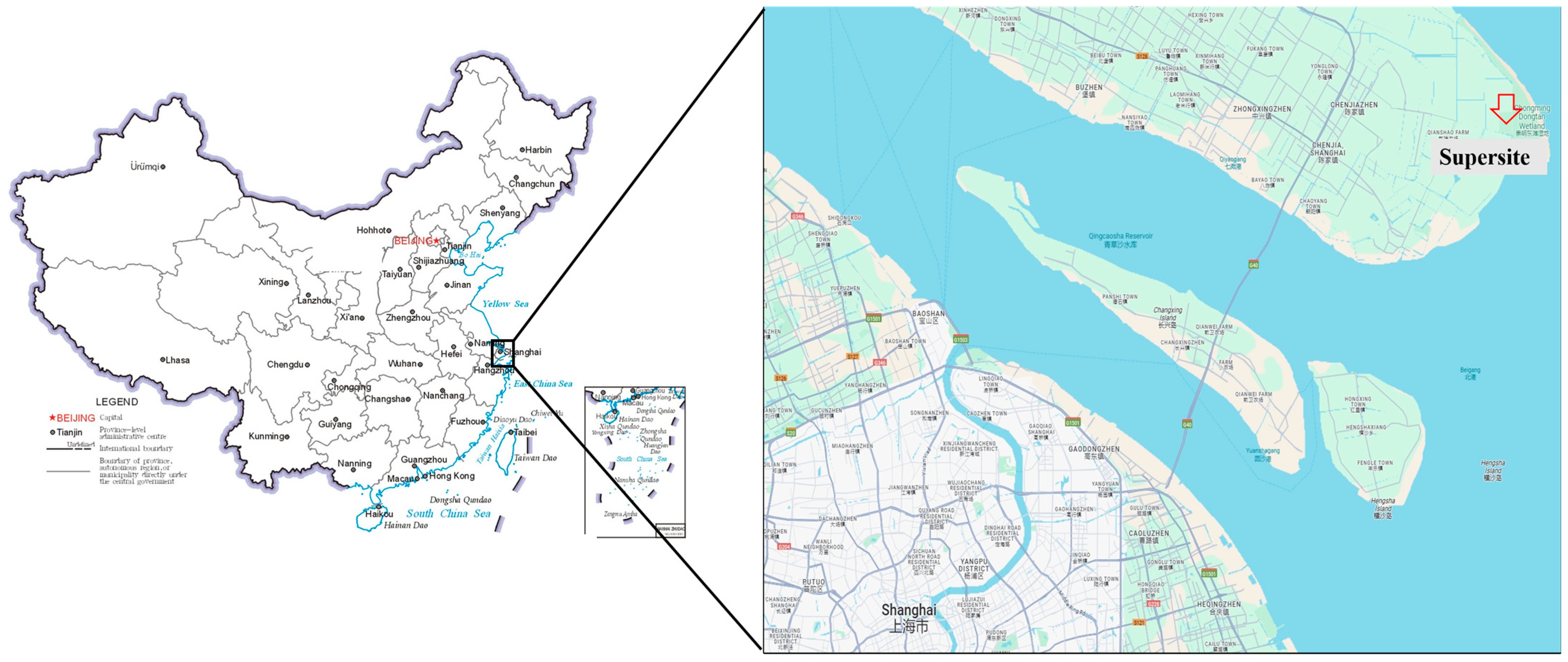
The data were collected from 1 January 2021 to 31 December 2021 at the Dongtan Supersite in Chongming District, Shanghai (31.51° N, 121.96° E). This is a typical island area, close to a megacity, near the ocean, with a relatively small population density. It belongs to the offshore environmental ecological zone close to the city, as shown in Figure 1. Multiple instruments were used to measure the hourly concentrations of PAN, NOx, O3, PM2.5, and 56 types of VOCs. Meteorological parameters include temperature, relative humidity [33], wind speed [34], and wind direction. The time resolution was 1 h.
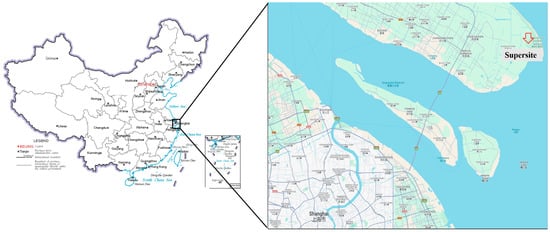
Figure 1.
Location of Shanghai Chongming Dongtan Supersite.
2.2. Random Forest Model
Random forest (RF) is an integrated supervised learning method that can be seen as an extension of the decision tree [35]. In this study, the RF prediction model was built using the “sklearn” package in Python (version 3.12). Prior to model training, we used Python’s Pandas (in combination with sklearn’s preprocessing tools) to identify and remove blank values and outliers, ensuring high-quality data for modeling. Specifically, blank values were removed using the ‘dropna()’ function, and outliers were detected and removed based on the Z-score method—data points with an absolute Z-score greater than 3 were considered outliers and excluded from the analysis. To obtain the optimal parameters for the model, GridSearch was employed to identify the best combination of parameters for the RF model. Ultimately, the optimal configuration consisted of 200 decision trees, with a maximum tree depth of 10. The dataset was split into 80% for training and 20% for testing. The model’s performance was evaluated by calculating the R2 (coefficient of determination) and RMSE (root mean square error) between the predicted and observed values. The model inputs included the concentrations of ‘Isoprene’, ‘Ethane’, ‘PAN’, ‘m/p-Xylene’, ‘Toluene’, ‘Propylene’, ‘o-Xylene’, ‘1-Butene’, ‘Ethylbenzene’, ‘n-Pentane’, ‘n-Butane’, ‘Propane’, ‘POC’, ‘SOC’, ‘PM2.5’, ‘temperature’, ‘relative humidity’, ‘wind speed, ‘wind direction’, ‘NOx’, and ‘PSA’. The output was the concentration of O3. The top ten VOCs were selected based on their O3 formation potential (OFP) ranking, which was calculated using the maximum incremental reactivity (MIR) method from a total of 56 VOCs. For a detailed explanation of the calculation method, please refer to the Supplementary Materials, Note S2, Table S2. The RF model provides two tools to estimate the importance of individual features: the mean squared error (MSE) increase and node purity increase. To enhance the robustness of feature importance, both metrics were converted into percentages to determine the final variable importance. The training dataset for the RF model included data on O3, PM2.5, NOx, SOC, POC, PSA, PAN, and VOCs from 1 January 2021 to 31 December 2021. Importantly, feature calculations were not performed in isolation but were fully integrated across all records in the observed dataset, ensuring the model reflects real-world meteorological diversity. A total of 6924 valid samples were obtained during this period, of which 5539 were used for training and 1385 for testing.
2.3. Feature Importance
The importance of features is determined by evaluating their impact on the model’s predictive performance using mean squared error (MSE) increment. The MSE increment method evaluates feature importance by calculating the increase in the model’s MSE after the features are randomly shuffled or removed. The greater the increase, the more important the feature [36].
SHAP (SHapley Additive exPlanations) is an explanation method based on game theory. It uses a theoretical method based on Shapley values to assign a specific estimated importance value to each variable and determines the individual and interactive effects of each variable on O3 formation from the optimal model. It treats each combination of features as a combination [37]. The SHAP value of a feature is calculated by averaging its marginal contribution across all alliances. The SHAP formula is shown below [38]:
denotes the prediction, is the base value (typically the average prediction over the dataset), and is the base value (typically the average prediction over the dataset) and represents the SHAP value for feature (), quantifying its contribution to the prediction.
2.4. RF-PDP Method
RF-PDP (random forest partial dependence plot) is a method that combines the RF model and a partial dependence plot (PDP) to analyze and visualize the impact of features on model predictions [39,40]. First, an RF model is trained to make predictions and evaluate the importance of features. Next, partial dependencies are calculated, that is, the value of a feature is changed while other features are fixed, and the average predicted value of the model is calculated [41]. Finally, these calculation results are visualized as partial dependency plots to show how the model’s predicted value changes when the feature value changes. The RF-PDP method provides a deep understanding of the relationship between features and predicted results by combining the nonlinear modeling capabilities of RF with the intuitive visualization of PDP, revealing the overall impact of features on predicted results.
The 3D partial dependence plot (3D-PDP) is a visualization tool used to explain the relationship between features and prediction targets in machine learning models. In research, 3D-PDP can help this study understand the impact of two features changing at the same time on the target variable [42]. In this study, this study used the 3D partial dependence plot (3D-PDP) to explore how changes in two features jointly affect O3 concentration. 3D-PDP enables this study to intuitively observe the response of the model to different feature combinations by displaying the relationship between features and predicted values in three-dimensional space. The 3D-PDP can reveal the interaction effect between two features and can also reveal the nonlinear relationship between features and target variables. The specific formula is as follows [10]:
Among them, means when the input is , The predicted value of the RF model; RF represents the trained RF model; is the feature selected when calculating the partial dependence function in the RF model; represents the features not selected in the RF model and is input into the model with a fixed value; and n represents the number of samples.
2.5. Structure Mining Method
Structural mining methods, specifically the minimum depth (min-depth) method, are a technique used to analyze tree-based models such as RF [43]. The method aims to quantify the importance of features by examining their structural position in the ensemble of decision trees that make up the model. It provides a measure of how early a particular feature is used to split the data within each tree. In the context of decision tree algorithms such as those used in RF, the minimum depth of a feature refers to the layer or depth at which the feature is first used as a decision criterion in the tree structure. More formally, the minimum depth of a feature ff in a decision tree is defined as the distance from the root node (depth = 0) to the first occurrence of ff in any node in the tree. This metric provides insight into the relative importance of features: features that are closer to the root (i.e., have a smaller minimum depth) are generally more influential in predicting the target variable. The main rationale behind minimum depth is that important features tend to be selected earlier in the tree building process because they provide the most information gain or impurity reduction at higher levels of the tree. Therefore, features with lower minimum depth values are considered more important because they contribute more to the predictive performance of the model.
The minimum depth method provides an interpretable and rigorous way to understand feature importance in RF models. By focusing on the depth of the first selected features, it provides a direct and intuitive measure of feature importance that complements traditional importance metrics.
2.6. Trajectory Concentration Clustering Calculation
The backward trajectory clustering method is used to study the potential transport pathways of pollutants. Backward trajectory analysis uses the global reanalysis database developed by NOAA Air Resources Laboratory [8]. This method can provide a comprehensive understanding of the transport and distribution of pollutants in relation to meteorological dynamics and atmospheric circulation patterns. Using the GBL format file from the official NOAA website, the Hybrid Single Particle Lagrangian Integrated Trajectory (HYSPLIT) module is used to generate the backward trajectory of the air mass [44]. Next, the cluster model was used to calculate pollutant concentrations using the geographic information system [45]-based TrajStat software (version 1.5.5) from Meteoinfo [46].
3. Results and Discussion
3.1. Time Series Analysis of O3 and Its Related Factors
By monitoring the hourly variations in O3 and its influencing factors at the Chongming Dongtan supersite in Shanghai from 1 January to 31 December 2021 (as shown in Figure 2), this study identified patterns in O3 concentrations based on long-term observations of atmospheric pollutants and meteorological parameters in the Chongming region. It was found that O3 concentrations were higher in both spring and autumn. Specifically, Figure 2a illustrates the seasonal variation of O3 alongside NOx, PM2.5, and PAN. O3 concentrations gradually increased during spring (March–May), slightly declined in summer, rose again in autumn, and dropped to their lowest levels in winter. This pattern is similar to findings from numerous coastal regions, where O3 concentrations in spring and autumn are higher than in summer [47,48]. In contrast to northern regions, where O3 peaks typically occur in summer, the highest concentrations in coastal areas are observed in spring and autumn [49]. This trend indicates that O3 formation is primarily driven by photochemical reactions, with significant increases in O3 production. The decline in O3 concentrations during summer can be attributed to the reduction in pollutant levels. NOx concentrations were higher during the winter months (December and January) and lowest in summer, likely due to increased fossil fuel combustion in winter and the rapid photochemical consumption of NOx in summer. The seasonal variation in PAN is closely correlated with that of PM2.5, suggesting a possible shared source. NOx in the atmosphere is involved in converting into nitrates to promote PM2.5 formation and also in PAN formation. The similar temporal characteristics of PAN and PM2.5 imply that PAN may share a similar origin with PM2.5. We will explore this further in the backward trajectory analysis later.
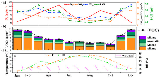
Figure 2.
Monthly variation patterns of O3, precursors, and meteorological conditions during the monitoring period. (a) O3, (b) VOCs, (c) Temperature.
Figure 2b illustrates the seasonal variation in different VOCs components, including alkanes, alkenes, aromatics, alkynes, and total VOC concentrations. The total concentration of VOCs peaks in winter and gradually declines through spring and summer. This seasonal variation reflects increased combustion activities in winter, coupled with poor atmospheric dispersion conditions. Alkanes constitute the largest proportion of total VOCs, particularly during winter, indicating that their primary source may be combustion emissions. Although alkenes, aromatics, and alkynes represent a smaller proportion, they make significant contributions to the formation of O3 and PAN. In summer, O3 levels decreased primarily due to relatively lower precursor concentrations of VOCs and NOx, as shown in Figure 2, while higher wind speeds, as indicated in Figure S2, facilitated the diffusion of these precursors, further contributing to the reduced O3 concentrations. The seasonal variation in VOCs is closely related to atmospheric photochemical reactions, particularly as they serve as precursors for O3 and PAN. The seasonal fluctuations of VOCs directly influence the formation processes of atmospheric pollutants.
Figure 2c presents the seasonal variations in temperature, relative humidity [33], and wind speed [34] throughout the year. The temperature peaks in summer and reaches its lowest levels in winter, displaying typical seasonal fluctuations. High temperatures promote photochemical reactions, thereby facilitating the formation of O3 and PAN. Relative humidity is higher in spring (around 80%) and lower in winter (approximately 60%), with humidity variations influencing the formation of particulate matter and the dispersion of pollutants. Wind speeds are lower in winter and slightly higher in summer. Elevated wind speeds assist in the dispersion and dilution of pollutants, whereas lower wind speeds can lead to pollutant accumulation, particularly in winter. In combination with higher humidity, lower wind speeds in winter may contribute to the accumulation of particulates such as PM2.5. The seasonal variations in temperature, relative humidity, and wind speed have a significant impact on pollutant concentrations, particularly in summer, when higher temperatures and wind speeds contribute to O3 formation and the dispersion of particulate matter.
The seasonal variations of O3, NOx, PM2.5, PAN, and VOCs are influenced by a combination of atmospheric photochemical reactions and meteorological conditions. The summer peaks in O3 and PAN are primarily driven by active photochemical reactions, with VOCs and NOx serving as precursors interacting under conditions of sunlight and high temperatures. The concentrations of NOx and PM2.5 are higher in winter, largely due to anthropogenic emissions and meteorological factors such as combustion emissions and poor atmospheric dispersion. VOC compositions are dominated by alkanes in winter, whereas in summer, they participate in atmospheric chemical reactions and are rapidly consumed, exacerbating O3 formation. The seasonal fluctuations in meteorological conditions (temperature, relative humidity, and wind speed) play a critical role in pollutant formation, dispersion, and deposition. In particular, the higher temperatures and wind speeds in summer facilitate the generation or dispersion of pollutants.
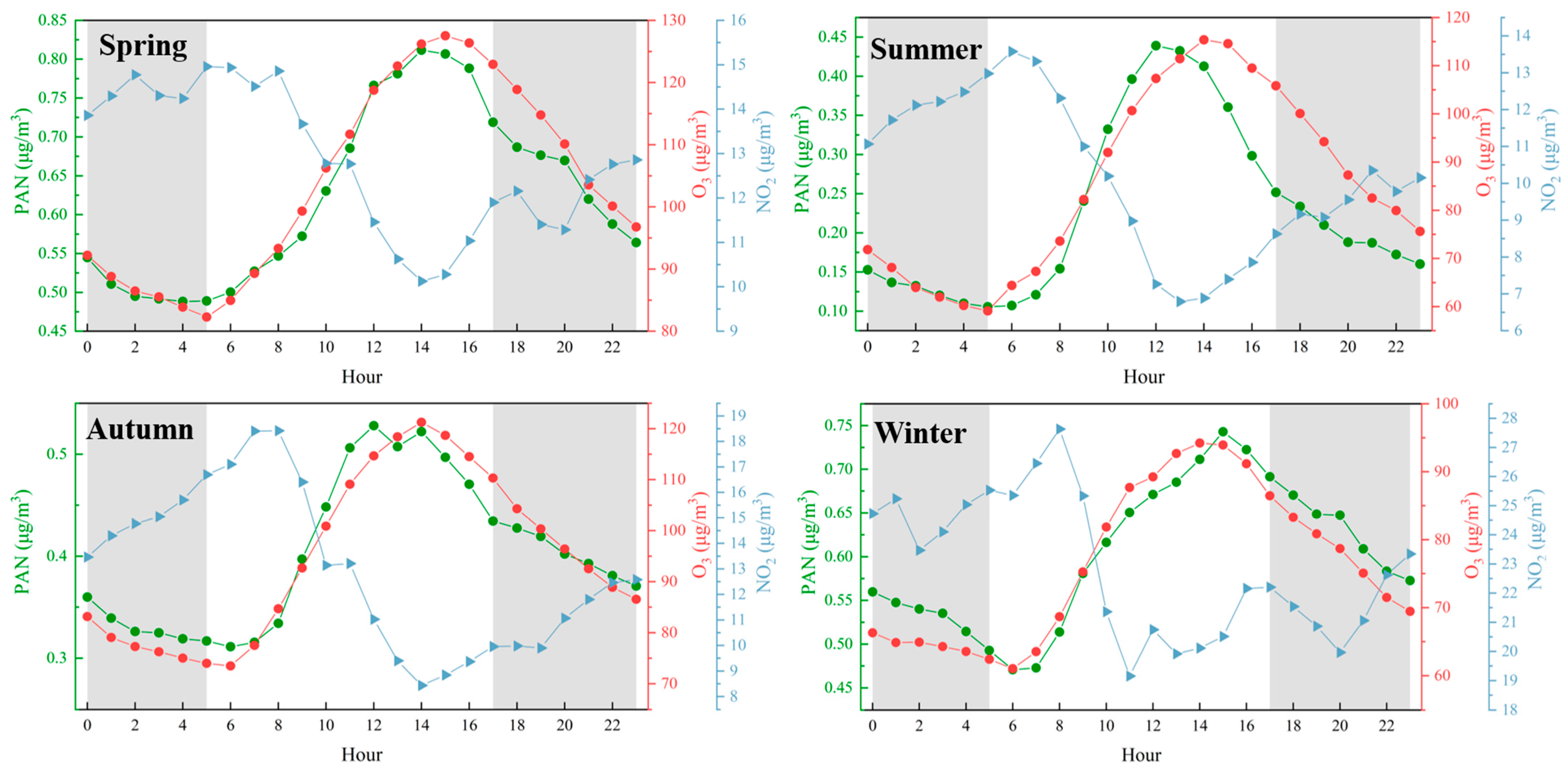
The seasonal analysis of PAN, O3, and NO2 concentrations reveals distinct temporal patterns across spring, summer, autumn, and winter. In spring, summer, and autumn, PAN concentrations peak between 10:00 and 12:00, reaching approximately 0.81 μg/m3, 0.44 μg/m3, and 0.53 μg/m3, respectively. In contrast, O3 concentrations exhibit a delayed peak between 14:00 and 16:00, with values of approximately 120 μg/m3, 130 μg/m3, and 120 μg/m3 for the same seasons. A similar pattern emerges in winter, where PAN peaks at around 0.75 μg/m3 between 10:00 and 12:00, followed by an O3 peak of approximately 90 μg/m3 between 14:00 and 16:00. This consistent 2–4 h lag between the PAN and O3 peaks suggests a potential mechanistic link between PAN decomposition and subsequent O3 formation.
As shown at Figure 3, the observed temporal relationship is consistent with known photochemical processes. PAN serves as a temporary reservoir for nitrogen oxides (NOx) and organic radicals, which are released upon its decomposition under conditions of elevated temperature and sunlight. This decomposition produces NO2 and RO2, both of which are critical precursors in O3 formation. The peak of PAN concentrations in the late morning, followed by elevated O3 levels in the early to mid-afternoon, supports the hypothesis that PAN decomposition contributes significantly to O3 production. Notably, this pattern persists across all seasons, indicating that the underlying photochemical mechanism is robust and not confined to specific seasonal conditions.
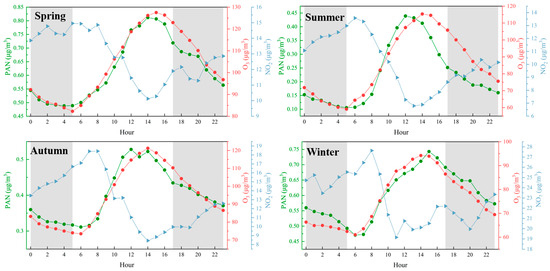
Figure 3.
Diurnal patterns of PAN, O3, and NO2 concentrations in different seasons, The red line represents O3, the blue line represents NO2, and the green line represents PAN. The shaded areas indicate nighttime periods.
While the data provide compelling evidence for the role of PAN in driving O3 formation, other factors warrant consideration. For example, the availability of VOCs plays a key role in radical cycling within photochemical systems and may enhance O3 production. Additionally, meteorological variables—such as temperature, relative humidity, and solar radiation—likely influence the rates of PAN decomposition and O3 formation. Nevertheless, the consistent lag between PAN and O3 peaks across multiple seasons suggests that PAN decomposition is a primary contributor to the observed O3 trends, even if modulated by these external factors.
These findings highlight the necessity of incorporating PAN into models of O3 formation, particularly in suburban environments where PAN concentrations are often elevated. Given its toxicity to human health and its role as a precursor to O3, a deeper understanding of PAN’s behavior and its interactions with O3 is essential for evaluating air quality and associated public health risks.
3.2. Model Performance and Feature Important
The dataset used in this study was obtained through the use of multiple instruments that measured the hourly concentrations of various atmospheric parameters. These parameters include PAN, NOx, O3, PM2.5, and VOCs. In addition, meteorological parameters such as temperature, relative humidity [33], wind speed [34], and wind direction [47] were also recorded.
Too many features may lead to overfitting of the model, so this study calculated the O3 formation potential (OFP) of all VOCs using the maximum incremental reactivity [27] method. Based on the OFP, 10 volatile organic compounds were selected as VOC features in descending order according to their OFP. These selected VOCs were then used as input features in the RF model.
In total, 6924 valid samples were obtained during this period. These samples were divided into two subsets: 5539 samples were used for training the model, while the remaining 1385 samples were reserved for testing. The training dataset was used to develop and fine-tune the RF model, enabling it to capture the relationships between the input variables (PAN, NOx, O3, PM2.5, selected VOCs, meteorological factors) and the target variable (O3 concentration). The test dataset was then employed to evaluate the model’s performance and generalizability. For more details on the observation instruments, please refer to the Supplementary Materials.
Based on the results shown in Figure S1, both random forest (RF) and XGBoost demonstrated high predictive accuracy for O3 concentration prediction. However, a closer examination revealed that RF exhibited a lower R2 variance (0.03335 for RF versus 0.04082 for XGBoost) and a slightly higher average R2 score, indicating more consistent performance across different cross-validation folds. In contrast, other models such as ANN, RNN, SVR, and KNN produced noticeably lower R2 values. Given the ecological sensitivity of the nearshore region under investigation, where robust and reliable predictions are critical, we ultimately selected random forest as the primary model for further analysis and interpretation.
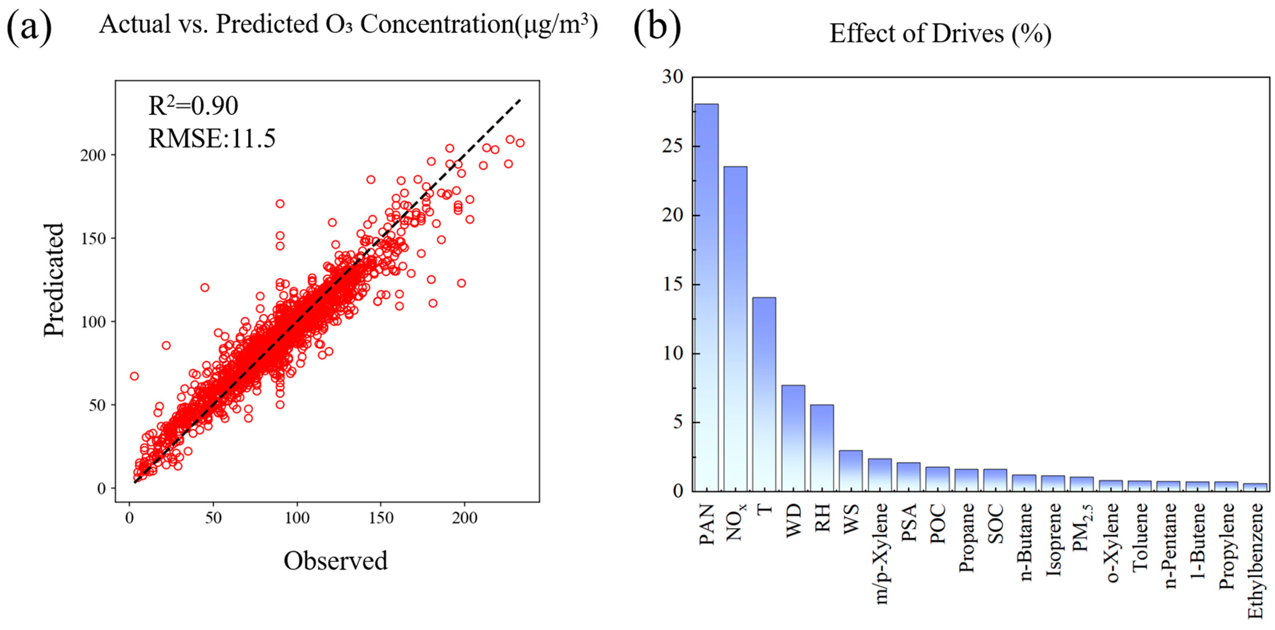
Figure 4a shows the comparison between the O3 concentration predicted by the RF model and the actual observations, and the results show that the model has good performance, with an R2 value of 0.90 and a root mean square error (RMSE) of 11.498. This indicates that the model has high accuracy in predicting O3 concentration. For a detailed model performance comparison, see the Supplementary Materials. The scatter plot of actual O3 concentration and model prediction values shows that most data points are closely distributed near the 1:1 line, especially in the medium and low concentration range (about 50–150 μg/m3), showing a strong linear correlation. This indicates that the model has high prediction accuracy. The research by Watson et al. (2019) [33] yielded analogous results when forecasting wildfire-related O3 exposure in California, with random forest demonstrating superior predictive capability among ten evaluated machine learning models. Zhan et al. (2018) [1] successfully applied random forest (RF) to predict O3 concentrations in China with high accuracy. RF is widely recognized for its strong predictive performance, particularly in capturing nonlinear relationships between input variables and the target output—a capability that distinguishes it from alternative methods such as support vector machines (SVMs) and neural networks [50,51]. However, there is a slight underestimation trend in the high concentration area (>150 μg/m3), which may be caused by the complexity and scarcity of extreme pollution events.
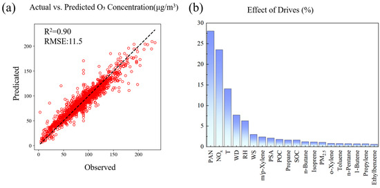
Figure 4.
Validation and analysis of O3 prediction model estimated as RF: (a) scatter plot of observed vs. predicted O3 concentrations with model performance metrics; (b) feature importance of drivers in O3 concentration prediction.
Feature importance analysis (Figure 4b) reveals the key factors affecting O3 concentration. PAN and NOx (nitrogen oxides) are identified as the most important predictors, followed by temperature, wind direction, and relative humidity [33]. This ranking emphasizes the combined role of precursors, meteorological conditions, and particulate matter in O3 generation. Yao et al.’s [52] RF-based O3 prediction study identified temperature and NOx as the most influential features through importance analysis, aligning broadly with our results. The dominance of NOx highlights the importance of controlling traffic and industrial emissions, while the higher importance of temperature illustrates the significant impact of climate factors on O3 pollution levels. Figure S3, which presents SHAP values, further supports this analysis. The SHAP plot is similar to the feature importance chart, but it reveals that NOx shows a negative effect on O3 when its concentration is high, and a positive effect when its concentration is low. This dynamic behavior of NOx emphasizes the complex relationship between precursor levels and O3 formation.
3.3. Partial Dependence Plot
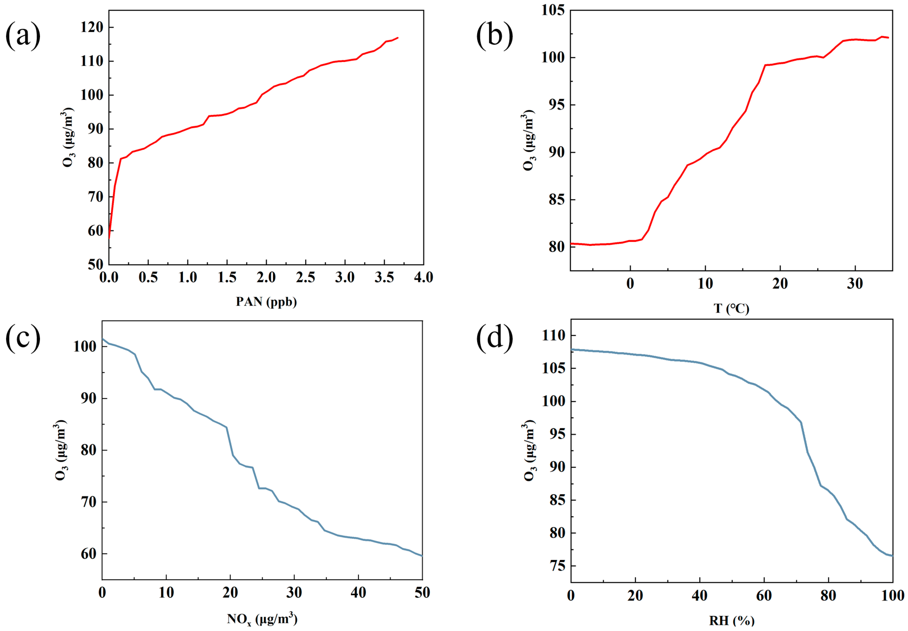
Based on the machine learning analysis using partial dependence plots (PDPs), the figure reflects the role of four key factors—PAN, temperature, NOx, and relative humidity [33]—in O3 generation. These figures, respectively, show the impact of each factor on O3 concentration changes within a specific range, from which we can identify how these factors affect O3 concentration and thus deduce their positive and negative effects in predicting O3 concentration.
Figure 5a shows that PAN has a strong positive effect on the production of O3. As PAN increases from 0 to about 3.5 ppb, O3 concentration rises from approximately 60 µg/m3 to around 110 µg/m3, suggesting that PAN contributes to O3 formation. While PAN and O3 are both products of VOC oxidation in the presence of NOx and may share similar variation characteristics, the observed trend from the PDP highlights that PAN, as a precursor, can indeed elevate O3 levels under certain conditions. Consistent with Liu’s findings, our analysis reveals that PAN contributes to O3 formation under NOx-rich conditions. As demonstrated in Figure 3 and Figure 5, the nocturnal increase in NOx concentrations leads to subsequent PAN-driven O3 enhancement, mirroring the mechanisms reported in Liu’s study [53].
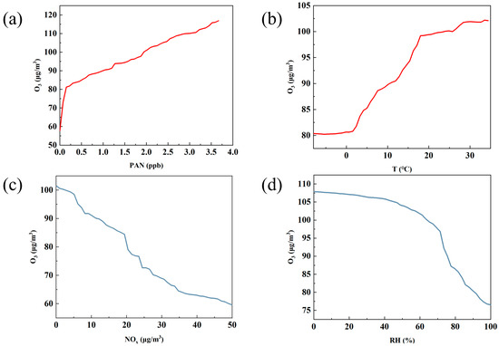
Figure 5.
Positive or negative (P/N) effects of individual drivers on O3 formation as estimated by RF-PDP. (a) PAN; (b) temperature; (c) NOx; (d) relative humidity [33].
Figure 5b shows the effect of temperature on O3 concentration. It can be seen from the figure that as the temperature increases, the O3 concentration gradually increases, showing an obvious positive effect. This is consistent with previous studies [54,55]. When the temperature increases from 10 °C to 30 °C, the O3 concentration increases from approximately 80 µg/m3 to over 100 µg/m3. This indicates that higher temperatures help promote the generation of O3, mainly because higher temperatures are usually accompanied by stronger solar radiation and more active photochemical reactions. This phenomenon is especially obvious in summer, because high temperature provides favorable conditions and accelerates the photochemical reaction rate of VOCs and NOx, resulting in a significant increase in O3 concentration. Therefore, temperature shows a positive contribution in O3 concentration prediction, especially in high-temperature seasons, when the impact is particularly significant.
Figure 5c shows the impact of NOx on O3 concentration, showing a typical negative correlation. As the NOx concentration increases from approximately 10 µg/m3 to 50 µg/m3, the O3 concentration gradually decreases from 100 µg/m3 to approximately 60 µg/m3. This negative correlation can be explained by the “NOx suppression effect”. When the NOx concentration is high, NO will react with O3 to generate NO2 and consume O3, thus inhibiting the generation of O3. When the NOx concentration is low, O3 generation is more active; however, when the NOx concentration is too high, O3 is consumed instead. This negative effect is especially obvious in urban areas with high NOx emissions, indicating that NOx is one of the keys limiting factors for O3 generation [45]. In the prediction model of O3, NOx usually shows a negative contribution, and its inhibitory effect on O3 increases as the concentration increases.
Figure 5d shows the effect of relative humidity [33] on O3 concentration, which also shows a negative effect. This is similar to previous studies [56]. As the relative humidity increases from 20% to 100%, the O3 concentration decreases from 110 µg/m3 to 80 µg/m3. High humidity conditions usually mean more cloud cover and weaker solar radiation, inhibiting photochemical reactions from occurring. In addition, high humidity helps the sedimentation of pollutants, further reducing O3 production. Therefore, increased humidity has a suppressive effect on O3 concentrations, which is particularly significant in humid climate conditions, especially during cloudy or rainy seasons. This shows that the influence of relative humidity contributes negatively to the prediction of O3, and higher humidity usually means a lower O3 production rate.
Similarly to Wang et al.’s [57] study using random forest for O3 prediction, our partial dependence plot (PDP) analysis of feature impacts on O3 concentrations revealed comparable patterns: temperature showed limited influence below 0 °C, and NOx exhibited increasing effects at higher concentrations. However, our study demonstrated a stronger impact of relative humidity [33] on O3 levels compared to Wang’s findings, which is potentially attributable to our study’s unique ecoregion characteristics.
Overall, these four variables show different directions of influence in the prediction of O3 concentration. PAN and temperature have significant positive contributions to O3 generation, while NOx and relative humidity have significant negative effects on O3 concentration. In model predictions, the combined effect of these factors reveals the complex change mechanism of O3 concentration, emphasizing the different impact paths of different meteorological conditions and precursors in the O3 generation process.
3.4. Feature Importance in Four Seasons
Since the response of O3 to different factors may vary by season, this study divides the months into different seasons, trains RF models for each season, and estimates the feature importance for each factor influencing O3 concentrations. Feature importance plots are then drawn to examine the response of O3 concentrations to different factors across the seasons.
In Figure 6, we observe the contributions of various chemical components and meteorological factors to the prediction of O3 concentrations in spring. Notably, temperature, relative humidity, NOx, and PAN all play significant roles in O3 formation. Among these, NOx is the largest contributing chemical factor in spring. Temperature and relative humidity also have key roles, which is closely related to the accelerated photochemical reaction rates and the influence of humidity on O3 generation. Changes in relative humidity notably impact O3 concentration prediction, while higher temperatures promote O3 formation [54,55]. It is worth noting that VOCs, such as ethylbenzene, n-pentane, and isoprene, contribute less in spring, likely due to the lower reactivity of VOCs under cooler conditions.
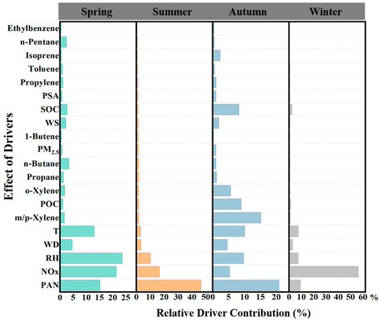
Figure 6.
Effects of individual drivers as estimated by variable importance analysis in each season.
In summer, the most significant contributor to O3 formation is PAN, followed by NOx and relative humidity. This result indicates that O3 concentrations in summer are primarily driven by high temperatures and photochemical reactions. The rise in temperature accelerates the decomposition of PAN, further intensifying O3 formation. Additionally, the longer and more intense sunlight during the summer provides abundant energy for O3 generation. Although relative humidity continues to contribute, its influence is weaker compared to spring.
As we transition to autumn, the influence of PAN on O3 concentrations becomes more pronounced. At the same time, m/p-Xylene also contributes to O3 formation. According to research by Xiao et al. [58], the main contribution of m/p-Xylene in Shanghai comes from fuel evaporation. Moreover, PAN still accounts for a significant portion of the contribution, indicating that precursor substances remain crucial for O3 formation. The photochemical reaction rate in autumn is slower than in spring and summer, so the dominant drivers of O3 formation shift toward chemical components rather than meteorological conditions.
In winter, the impact of drivers on O3 formation differs significantly from the previous seasons. The contribution of NOx sharply increases and becomes the most important factor, likely due to the lower temperature and reduced VOC reactivity in winter. Furthermore, the contribution of PM2.5 increases in winter, potentially due to the higher particle emissions from heating activities, which indirectly affect O3 formation. It is important to note that meteorological factors have a minimal effect on O3 in winter, suggesting that under low-temperature and weak-light conditions, O3 formation is primarily controlled by chemical precursors (especially NOx) and particulate matter. The contribution of VOCs, such as ethylbenzene and isoprene, is negligible in winter, further emphasizing their limited chemical reactivity under low-temperature conditions.
Overall, seasonal variations have a clear impact on the main drivers of O3 concentrations. In spring, summer, and autumn, PAN is consistently the dominant driver of O3 formation, followed by meteorological factors and NOx [54,55]. This result is in line with the typical mechanism of O3 generation, which is driven by photochemical reactions. In the hot and bright summer months, meteorological conditions dominate O3 formation, while in the colder seasons, O3 generation is more dependent on the supply of precursor substances. For pollution control, O3 emission reduction measures should focus on different aspects in different seasons. For example, in summer, emphasis should be placed on controlling O3 formation driven by meteorological factors, while in autumn and winter, reducing emissions of NOx, VOCs, and other precursor substances should be prioritized.
3.5. Two-DimensionalPartial Dependence Plot of Four Seasons
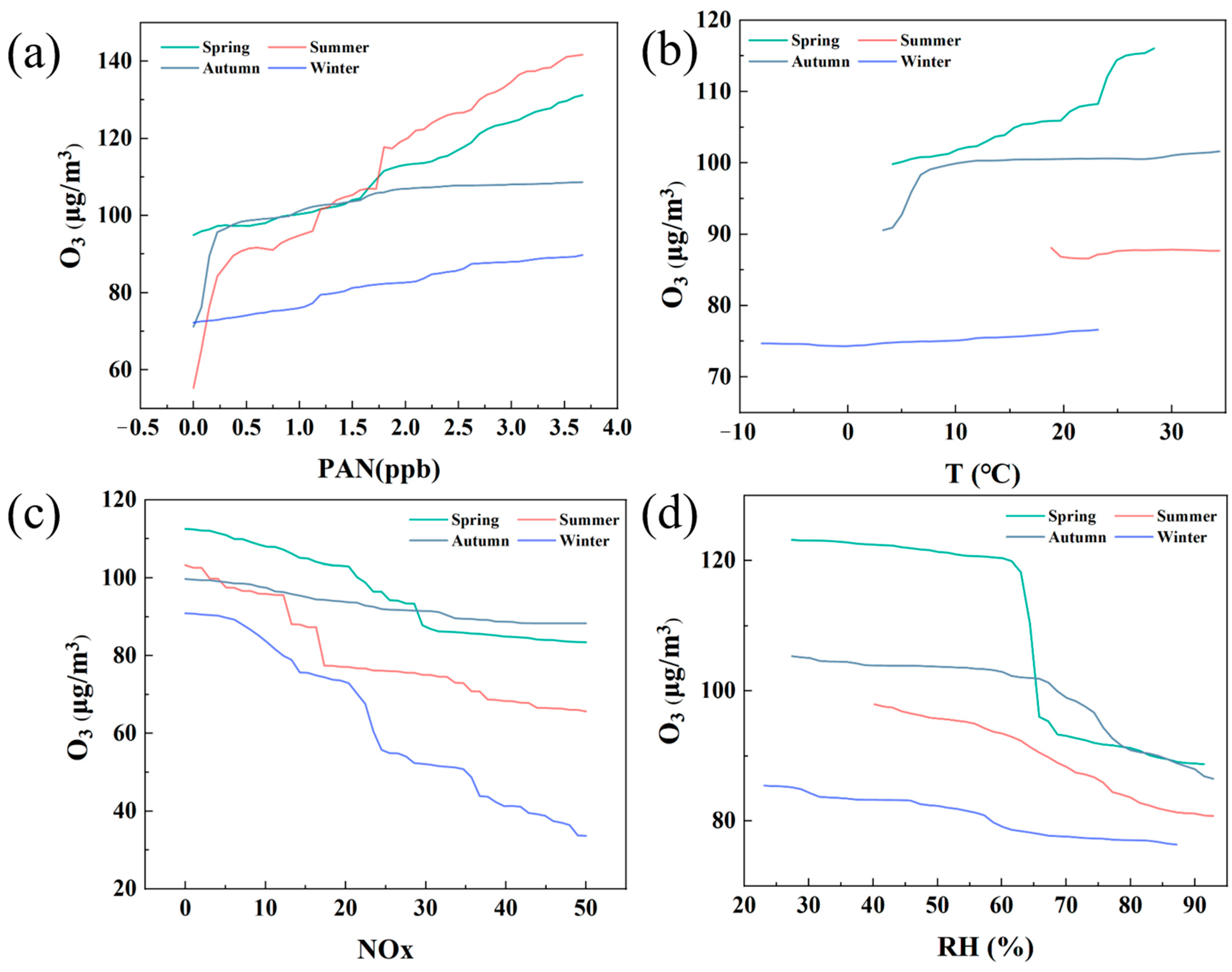
Figure 7 shows the influence of different meteorological factors and pollutants on O3 concentration by 2D-PDP analysis and compares them in spring, summer, autumn, and winter. Overall, the generation of O3 is closely related to season, precursor substances (such as PAN and NOx) and meteorological factors (such as temperature and relative humidity), and their influences show significant differences in different seasons.

Figure 7.
Positive or negative (P/N) effects of PAN, temperature, NOx, and relative humidity on O3 formation as estimated by RF−PDP. (a) PAN; (b) Temperature; (c) NOx; (d) Relative humidity.
Firstly, Figure 7a shows the influence of PAN concentration on O3 generation. In all seasons, the increase in PAN concentration leads to an increase in O3 concentration, but this upward trend is most significant in summer. This can be attributed to the fact that under the conditions of abundant sunshine and high temperature in summer, PAN, as a product of photochemical reaction, greatly promotes the generation of O3. Especially in summer, the O3 concentration rises rapidly with the increase in PAN, reflecting the strong driving effect of summer photochemical reaction. In contrast, the O3 concentration in winter is lower and less affected by the change in PAN, which reflects the characteristics of insufficient light and inactive photochemical reaction in winter.
Secondly, temperature, as another important meteorological factor, its influence on O3 generation is reflected in Figure 7b. The O3 concentration increased significantly with the increase in temperature in spring and autumn, especially in spring, where the increase in temperature was most closely related to the increase of O3 concentration. This indicates that the photochemical reaction in spring is more active, and the increase in temperature promotes the transformation of precursor substances and the generation of O3. However, the O3 concentration changes more slowly in summer and winter, especially in summer. Although high temperature is a favorable condition for the generation of O3, at a certain temperature, the O3 concentration no longer increases significantly due to other inhibitory factors (such as high humidity or the saturation effect of NOx). Similarly, the O3 concentration in winter does not increase significantly with the change in temperature, indicating that the photochemical reaction is limited in winter. Figure 7c shows the effect of NOx concentration on O3. In all seasons, the increase in NOx leads to a decrease in O3 concentration, especially in winter. This phenomenon can be attributed to the so-called “NOx saturation” effect, that is, when the NOx concentration is too high, it will not only not promote the generation of O3 but will reduce its concentration by reacting with O3. In winter, due to the weak photochemical reaction, the increase in NOx will significantly inhibit the generation of O3. In contrast, although O3 concentrations also decreased in spring and autumn, the negative effects of NOx were not as significant as in winter due to moderate sunlight and temperature. Figure 7d shows the effect of relative humidity on O3 generation. In all seasons, an increase in relative humidity will lead to a decrease in O3 concentration, especially in spring and autumn, when the humidity exceeds 60%, the O3 concentration decreases significantly. This may be because O3 in the atmosphere is more easily removed under high humidity conditions, thereby reducing its concentration. In addition, increased humidity may also inhibit the occurrence of photochemical reactions, further reducing the generation of O3. The O3 concentration in winter was originally low and did not change much with humidity, indicating that humidity had a limited effect on O3 in winter.
In summary, the figure reveals the sensitivity of O3 concentration to multiple driving factors in different seasons. In summer, the increase in PAN and temperature significantly promoted the generation of O3, while NOx and relative humidity had an inhibitory effect on it. In winter, the effect of NOx was the most significant, and high concentrations of NOx significantly inhibited the generation of O3, while humidity had little effect on O3. Spring and autumn are relatively balanced seasons, with O3 concentrations rising when temperature and PAN increase, but high humidity or NOx concentrations also inhibit their production. This seasonal difference reveals the complexity of the O3 generation mechanism and emphasizes the need to develop O3 pollution control strategies for different seasons.
3.6. Three-DimensionalPartial Dependence Plot
Figure 8 shows the predicted impact of different combinations of factors on O3 concentration through 3D-PDP analysis. The four sub-graphs in the figure, respectively, combine different meteorological and pollutant factors in binary form to explore their synergistic effects on O3 generation. The color represents the O3 concentration, and the color scale changes from light blue (low concentration) to orange (high concentration), which illustrates the trend of O3 concentration under specific conditions. From these charts, it can be seen that O3 concentration is affected by multiple factors, and the change pattern of O3 concentration under different combinations of factors shows significant differences.
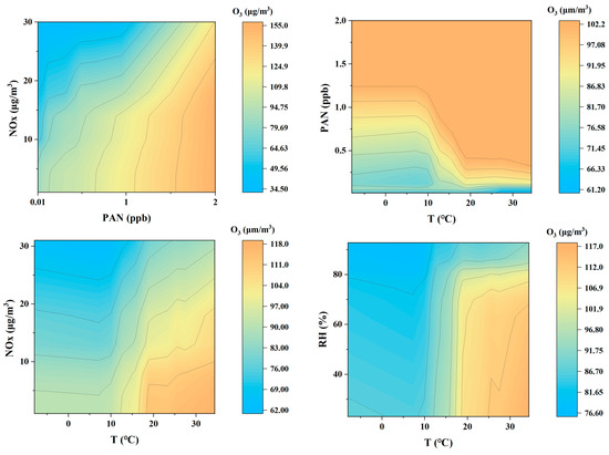
Figure 8.
Four pairs of interactions displayed through RF-3Dpdp.
First, the interaction between PAN and NOx on O3 concentration. Overall, as the concentrations of PAN and NOx increase, the concentration of O3 also increases. This is similar to previous studies [53]. In particular, when the concentration of PAN gradually increases from 0.01 ppb, the concentration of O3 increases rapidly, indicating that PAN significantly promotes the generation of O3 under high NOx concentration conditions. This is consistent with the characteristics of PAN as a photochemical reaction product, and PAN can accelerate the generation of O3 in a high NOx environment. This phenomenon shows that PAN and NOx have a synergistic effect in the generation of photochemical smog, especially in areas with more serious pollution. When NOx and PAN increase at the same time, the O3 concentration may rise sharply, leading to more serious photochemical pollution events.
From the synergistic effect of temperature and PAN concentration on O3. It can be seen that under higher PAN concentrations (1–2 ppb) and higher temperatures (20–30 °C), the O3 concentration increases significantly. This shows that high temperature and high PAN concentration jointly promote the generation of O3, especially when the temperature exceeds 20 °C, the O3 concentration rises rapidly, indicating that the photochemical reaction under high temperature conditions is very active. Elevated temperatures accelerate the thermal degradation of PAN, thereby enhancing photochemical reaction rates and subsequently increasing O3 concentrations [53]. However, at low PAN concentrations (less than 1 ppb), the O3 concentration does not change much with increasing temperature. This may be due to insufficient reactants at low PAN concentrations, which cannot fully promote the generation of O3, so the change in temperature has limited effect on the O3 concentration. This shows that PAN concentration is a prerequisite for temperature-driven O3 generation.
The interaction between NOx and temperature found that at lower NOx concentrations, increased temperature significantly promoted O3 generation [59], especially when NOx concentration was less than 10 µg/m3, and increased temperature significantly increased O3 concentration. However, as NOx concentration increased to nearly 30 µg/m3, O3 concentration showed a downward trend regardless of temperature changes and could not be reversed even under high temperature conditions. This suggests that under high NOx concentrations, a “NOx suppression effect” may occur, that is, excessive NOx will react with O3, resulting in a decrease in O3 concentration. This result highlights the complexity of the effect of temperature on O3 generation under high NOx conditions, indicating that a single control of temperature is not sufficient to effectively reduce O3 pollution in a highly polluted environment.
Finally, the lower right figure shows the effect of relative humidity and temperature on O3 concentration. It can be seen that under higher temperature conditions (20–30 °C), the increase in humidity has a significant inhibitory effect on O3 concentration, and when humidity exceeds 60%, the O3 concentration decreases significantly. This may be because the presence of water vapor under high humidity conditions accelerates the scavenging reaction of O3 or inhibits the photochemical reaction of precursor substances, thereby reducing the generation of O3. On the other hand, under low temperature conditions (less than 10 °C), the effect of humidity on O3 concentration is relatively gentle, indicating that temperature is the key factor determining the generation of O3, while the effect of humidity is mainly reflected in the inhibitory effect on O3 concentration under high temperature conditions.
In summary, this figure reveals the effect of the interaction of different meteorological factors and pollutants on O3 concentration through the 3D-PDP method. High temperature, low humidity, higher PAN, and moderate NOx concentration help promote the generation of O3, while high humidity and high NOx concentration have the effect of inhibiting the generation of O3. These findings provide important insights into the formation mechanism of O3 pollution and emphasize the need to consider the interaction of multiple factors when controlling O3 pollution, especially to formulate targeted response strategies under different meteorological and pollution conditions.
3.7. Min Depth
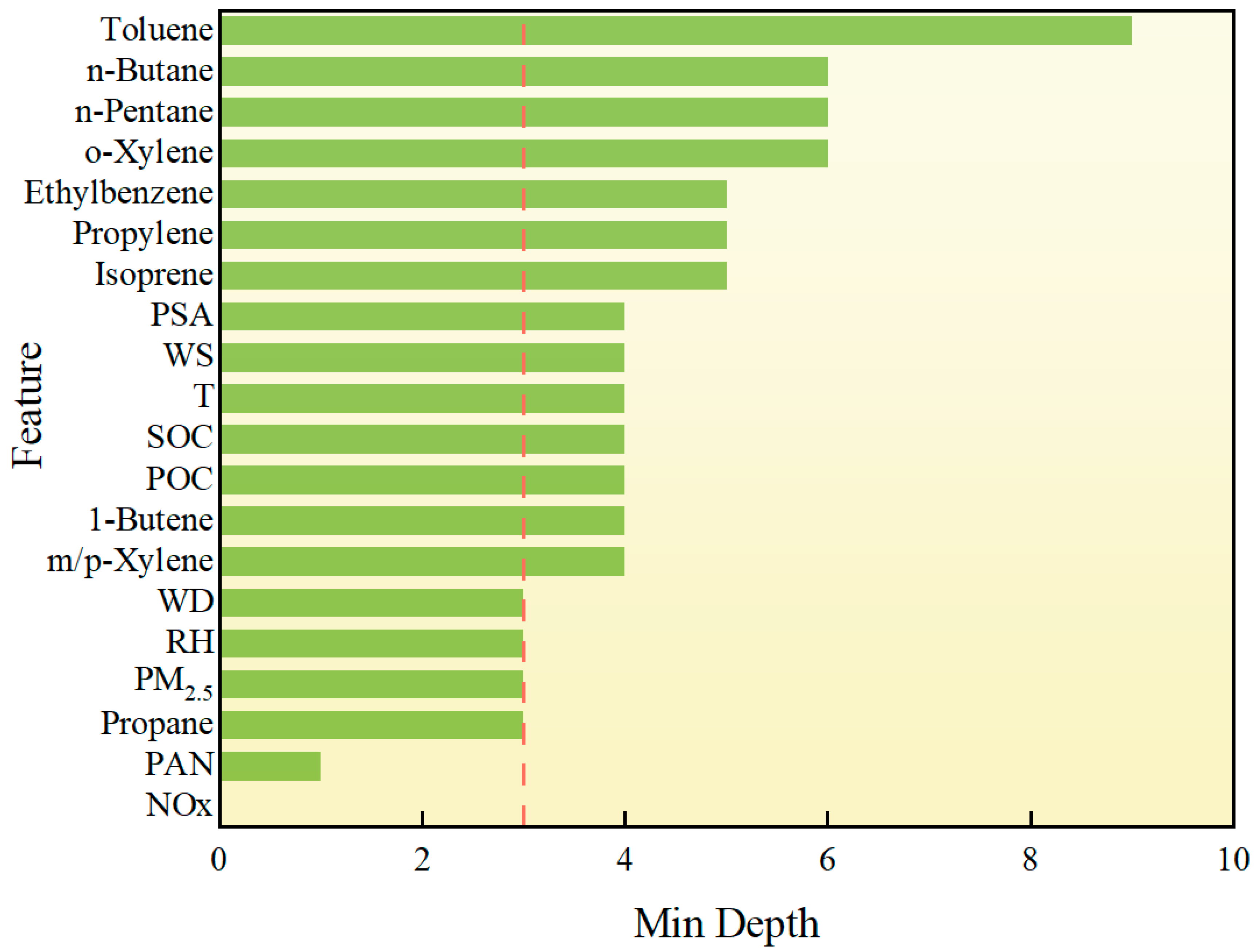
The above RF-based analysis of O3 drivers briefly illustrates their respective impacts. Since O3 is affected by multiple complex drivers, the interaction between multiple drivers also plays a vital role in the formation of O3. Therefore, it is necessary to study the different factors. Although RF cannot be directly used to study the interaction between paired drivers, exploring the structure of RF decision trees can help extract information from different factors. The main method of this structural mining analysis is based on the concept of minimum depth, that is, the minimum distance from the depth of a factor to the root of the tree. The minimum depth is within 3, which represents a strong contribution to the prediction of O3. For a single factor, if its MD is shallow, it is considered to be more important for the prediction of O3. As shown in Figure 9, in the minimum depth analysis of the RF model, NOx, and PAN are the most important features for predicting O3 concentration. The same as the previous feature importance and SHAP analysis. Although PAN itself is a secondary pollutant, it has a far-reaching impact in atmospheric chemistry, especially through its thermal decomposition to release NOx, which continues to affect O3 production. In addition, as one of the VOCs, propane also has a relatively low minimum depth, showing its greater contribution in the model. This is attributed to the reaction of propane with OH· in the atmosphere to form PAN precursors. Although PM2.5 (fine particulate matter) has a complex relationship with O3 generation, it can indirectly affect O3 concentration by adsorption, scattering, or changing the chemical environment in the atmosphere. The effects of meteorological factors such as relative humidity [33] and wind direction on O3 generation are more reflected in the transmission and diffusion of pollutants. For example, changes in wind direction may affect the accumulation and dilution of pollutants between regions, while humidity can inhibit the occurrence of certain photochemical reactions and indirectly reduce O3 generation.
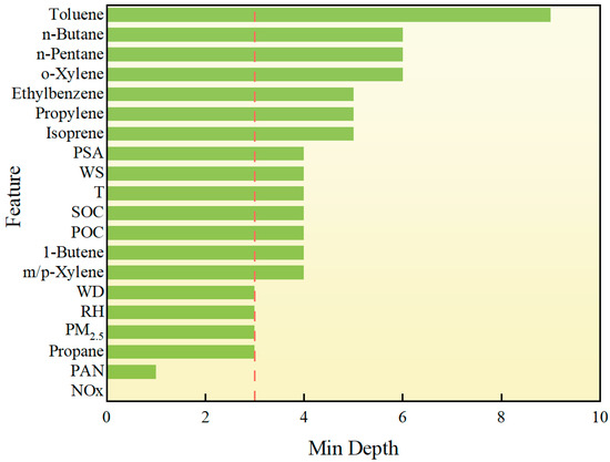
Figure 9.
Structure mining analysis of drivers. The red dashed line indicates features with a minimum depth < 3, suggesting higher relevance.
For the effect of temperature, although temperature is one of the variables with a more significant impact on O3 concentration in the previous feature importance and SHAP value analysis, its importance is lower in this minimum depth analysis. This phenomenon may be caused by a variety of factors. First, NOx and PAN show a stronger dominant role in the model, especially in the atmospheric photochemical reaction chain, where NOx is directly related to O3 production, while temperature indirectly affects O3 production mainly by regulating the reaction rate. Therefore, although temperature has an impact on atmospheric reactions, its effect may be more indirect than that of NOx and PAN, resulting in a relatively large minimum depth. Secondly, the RF model is able to capture the complex nonlinear interactions between features, and temperature may have a strong interactive effect with other meteorological variables (such as humidity or wind speed), resulting in a small contribution of temperature alone, but it is still important in the overall impact. The feature importance and SHAP value focus more on the direct impact of quantitative variables on the prediction results and may ignore the complexity of this interaction to a certain extent. This shows that although temperature still has an impact that cannot be ignored in O3 prediction.
3.8. Backward Trajectory Concentration Clustering
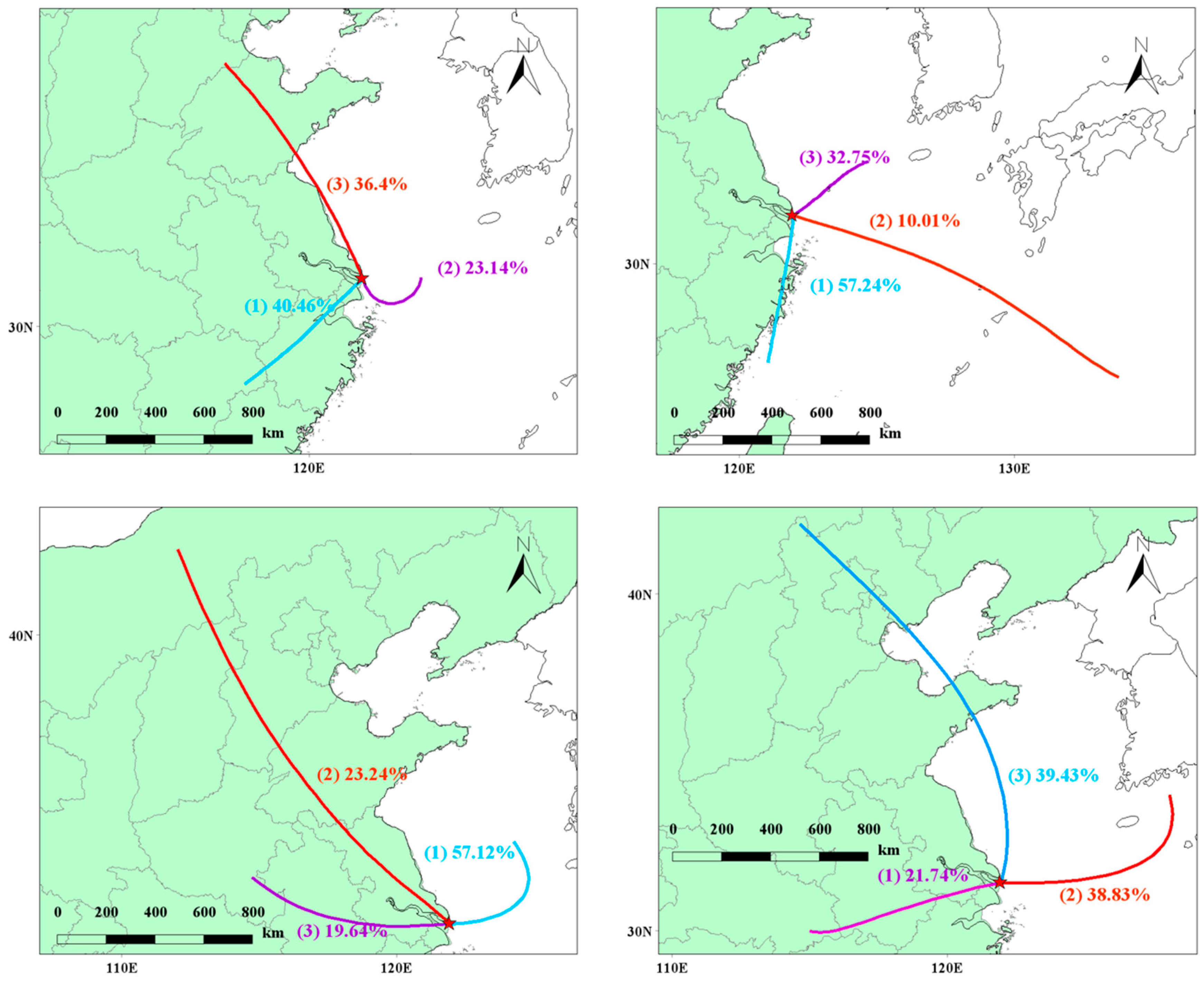
The trajectory clustering is shown in Figure 10, and the pollutant concentration clustering table is shown in Table 1. Starting from spring, the air mass clustering shows that the airflow from the inland southwest (passing through the Shanghai urban area) accounts for 40.46%, the airflow from the eastern sea direction accounts for 23.14%, and the northward airflow passing through the Shandong Peninsula along the Chinese coastline to Chongming accounts for 36.4%. The clustering analysis of pollutant concentrations reveals that the main sources of PAN and O3 are located in the inland and marine directions. This suggests that the primary pollution in Chongming Dongtan originates from Shanghai city and from the marine direction. Unlike local sources in Chongming, nitrogen oxides (NOx) emitted by ships have a positive effect on O3 generation in the marine area farther from the land. Furthermore, time series analysis shows that the variation trends of PM2.5 and PAN are similar, indicating that PAN and PM2.5 may share common sources, and PAN is likely to originate from long-range transport.
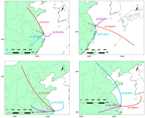
Figure 10.
Seasonal clustered trajectories over the observed site.

Table 1.
Pollutant concentration under airflow clustering.
In summer, the prevailing wind direction (Class I) is from the south of Chongming, accounting for 57.24%, passing through the Jinshan Chemical Park in Shanghai before reaching Chongming. Class II and III wind directions account for 10.01% and 32.75%, respectively, and both come from the sea. Notably, the main contribution to PAN is a result of Class I winds, especially those passing through the Jinshan Chemical Park in Shanghai. In addition, the O3 concentration contribution is higher under Class II winds, further confirming that ship emissions from the sea lead to an increase in O3 levels, which are then transported to Chongming Dongtan.
In autumn, the dominant wind direction remains the sea breeze, with Class I winds from the sea accounting for 57.12%. For this wind direction, PAN and O3 concentrations are generally higher, which further demonstrates that PAN contributes positively to the O3 levels in Chongming Dongtan after being transported from a distance. In winter, inland winds account for only 21.74%. Although PAN concentrations are higher under Class I winds, its effect on O3 concentration increase is limited due to low temperatures. However, Class II and III winds account for nearly 80%, and the O3 clustering concentrations are 87.5 μg/m3 and 88.83 μg/m3, respectively. This suggests that O3 generation in winter primarily originates from the sea and is transported long-distance, significantly influencing O3 levels in Chongming Dongtan. PAN’s promoting effect on O3 generation may exist in certain seasons (such as spring and autumn), but in other seasons (such as summer and winter), its effect may be regulated by other atmospheric factors. Therefore, it can be inferred that the role of PAN in O3 generation is seasonal and condition-dependent, rather than a simple co-transport relationship. According to the results of machine learning, PAN contributes the most to O3 in summer, indicating that under high-temperature conditions in summer, the life of PAN is reduced and it decomposes into NOx and VOCs, resulting in a higher contribution to O3 generation than in other seasons. Additionally, considering the backward trajectory analysis, it is believed that the transport of O3 from the ocean to Chongming Dongtan affects the local O3 concentration, but the high concentration of NOx in the local area has a negative impact on O3 generation.
In summary, although ship emissions play a leading role in the generation of O3 in spring and summer, especially in high-temperature and strong-light conditions, NOx emitted by ships generates a large amount of O3 through photochemical reactions; urban emissions are also not to be ignored, especially in autumn and winter, when urban emissions contribute significantly to pollutants such as PAN and PM2.5. This seasonal difference reveals the combined effect of ship and urban emission sources on the concentration of atmospheric pollutants.
4. Conclusions
In this study, we employed an interpretable random forest model to investigate the key factors influencing O3 concentrations in the Chongming region of Shanghai, with a focus on the complex interactions among precursors and meteorological conditions. The model demonstrated high predictive accuracy (R2 = 0.9), and feature importance analysis identified PAN, NOx, temperature, and relative humidity as primary drivers of O3 formation. Our analysis revealed clear seasonal patterns, with peak O3 levels in spring, and uncovered complex, nonlinear relationships between O3 and its precursors. Notably, while temperature and NOx were positively correlated with O3, NOx exhibited a dual effect—enhancing O3 formation at lower concentrations while inhibiting it at higher concentrations, particularly in summer due to intensified photochemical reactions. Relative humidity above 60% suppressed O3 formation, underscoring the intricate interplay between chemical and physical processes. Structural mining further confirmed that NOx and PAN significantly contribute to rising O3 levels. Backward trajectory clustering revealed that the remote transport of PAN and O3 from marine and urban industrial sources plays a critical role in the pollution observed on Chongming Island. These findings highlight the combined influence of precursor emissions and meteorological factors on O3 pollution, emphasizing the need for temperature-specific, multi-dimensional, and seasonally adjusted pollution management strategies. Overall, while our results are consistent with previous studies on the dual role of NOx and the positive influence of temperature, this work advances our understanding by elucidating the complex interactions between meteorological conditions and precursor emissions, particularly in ecologically sensitive wetland regions.
Supplementary Materials
The following supporting information can be downloaded at: https://www.mdpi.com/article/10.3390/atmos16040457/s1. Figure S1: Performance testing of different models for prediction, Figure S2 Comparison of wind speed at day and at night across four seasons, Figure S3 Individual sample impact of each driver on O3 as estimated by RF-SHAP; Table S1 Observed volatile organic compounds (VOCs) list Table S2 Calculated OFP of VOCs [60,61,62,63,64]. Supplementary Note S1. List of Abbreviations and Acronyms; Supplementary Note S2. Monitoring Instruments; Supplementary Note S3. Observed Volatile Organic Compounds (VOCs) List; Supplementary Note S4. Performance Testing of Different Models for Prediction; Supplementary Note S5. Calculation of OFP of VOCs Chemistry; Supplementary Note S6. Calculation of SOC, POC, and PSA; Supplementary Note S7. Method of Random Forests; Supplementary Note S8. Effects of Drivers as Estimated by RF-SHAP; Supplementary Note S9. Comparison of Wind Speed at Day and at Night across Four Seasons.
Author Contributions
Y.L.: data curation, formal analysis, investigation, validation, writing—original draft, writing—review and editing; T.H.: conceptualization, funding acquisition, methodology, project administration, supervision, writing—review and editing; Y.D. conceptualization, methodology, supervision; J.D.: investigation, writing—original draft. All authors have read and agreed to the published version of the manuscript.
Funding
This work was supported by the National Key Research and Development Program of China (no. 2022YFC3703500) and the financial support of the National Natural Science Foundation of China (51508395).
Institutional Review Board Statement
Not applicable.
Informed Consent Statement
Not applicable.
Data Availability Statement
The original contributions presented in this study are included in the article/Supplementary Material. Further inquiries can be directed to the corresponding author(s).
Conflicts of Interest
The authors declare that they have no known competing financial interests or personal relationships that could have appeared to influence the work reported in this paper.
References
- Zhan, Y.; Luo, Y.; Deng, X.; Grieneisen, M.L.; Zhang, M.; Di, B. Spatiotemporal prediction of daily ambient ozone levels across China using random forest for human exposure assessment. Environ. Pollut. 2018, 233, 464–473. [Google Scholar] [CrossRef] [PubMed]
- West, J.J.; Smith, S.J.; Silva, R.A.; Naik, V.; Zhang, Y.; Adelman, Z.; Fry, M.M.; Anenberg, S.; Horowitz, L.W.; Lamarque, J.-F. Co-benefits of mitigating global greenhouse gas emissions for future air quality and human health. Nat. Clim. Change 2013, 3, 885–889. [Google Scholar] [CrossRef] [PubMed]
- Wang, F.; Qiu, X.; Cao, J.; Peng, L.; Zhang, N.; Yan, Y.; Li, R. Policy-driven changes in the health risk of PM2.5 and O3 exposure in China during 2013–2018. Sci. Total Environ. 2021, 757, 143775. [Google Scholar] [CrossRef]
- Bureau, S.E.E. Shanghai Municipal Ecological Environment Bulletin in 2022; Shanghai Municipal Bureau of Ecology and Environment: Shanghai, China, 2022.
- Liu, P.; Song, H.; Wang, T.; Wang, F.; Li, X.; Miao, C.; Zhao, H. Effects of meteorological conditions and anthropogenic precursors on ground-level ozone concentrations in Chinese cities. Environ. Pollut. 2020, 262, 114366. [Google Scholar] [CrossRef] [PubMed]
- Yang, Y.; Liu, X.; Zheng, J.; Tan, Q.; Feng, M.; Qu, Y.; An, J.; Cheng, N. Characteristics of one-year observation of VOCs, NOx, and O3 at an urban site in Wuhan, China. J. Environ. Sci. 2019, 79, 297–310. [Google Scholar] [CrossRef]
- Koppmann, R. Chemistry of volatile organic compounds in the atmosphere. In Hydrocarbons, Oils and Lipids: Diversity, Origin, Chemistry and Fate; Springer: Berlin/Heidelberg, Germany, 2020; pp. 811–822. [Google Scholar]
- Juráň, S.; Karl, T.; Ofori-Amanfo, K.K.; Šigut, L.; Zavadilová, I.; Grace, J.; Urban, O. Drought Shifts Ozone Deposition Pathways in Spruce Forest from Stomatal to Non-Stomatal Flux. Environ. Pollut. 2025, 372, 126081. [Google Scholar] [CrossRef]
- Wang, T.; Xue, L.; Brimblecombe, P.; Lam, Y.F.; Li, L.; Zhang, L. Ozone pollution in China: A review of concentrations, meteorological influences, chemical precursors, and effects. Sci. Total Environ. 2017, 575, 1582–1596. [Google Scholar] [CrossRef]
- Xu, H.; Yu, H.; Xu, B.; Wang, Z.; Wang, F.; Wei, Y.; Liang, W.; Liu, J.; Liang, D.; Feng, Y.; et al. Machine learning coupled structure mining method visualizes the impact of multiple drivers on ambient ozone. Commun. Earth Environ. 2023, 4, 265. [Google Scholar] [CrossRef]
- Sun, M.; Zhou, Y.; Wang, Y.; Zheng, X.; Zhang, D.; Zhang, J.; Zhang, R. Seasonal discrepancies in peroxyacetyl nitrate (PAN) and its correlation with ozone and PM2. 5: Effects of regional transport from circumjacent industrial cities. Sci. Total Environ. 2021, 785, 147303. [Google Scholar] [CrossRef]
- Roberts, J.M. PAN and related compounds. In Volatile Organic Compounds in the Atmosphere; Wiley-Blackwell: Hoboken, NJ, USA, 2007; pp. 221–268. [Google Scholar]
- Moxim, W.; Levy, H.; Kasibhatla, P. Simulated global tropospheric PAN: Its transport and impact on NOx. J. Geophys. Res. Atmos. 1996, 101, 12621–12638. [Google Scholar] [CrossRef]
- Temple, P.; Taylor, O. World-wide ambient measurements of peroxyacetyl nitrate (PAN) and implications for plant injury. Atmos. Environ. 1983, 17, 1583–1587. [Google Scholar] [CrossRef]
- Zeng, L.; Fan, G.-J.; Lyu, X.; Guo, H.; Wang, J.-L.; Yao, D. Atmospheric fate of peroxyacetyl nitrate in suburban Hong Kong and its impact on local ozone pollution. Environ. Pollut. 2019, 252, 1910–1919. [Google Scholar] [CrossRef] [PubMed]
- Aneja, V.P.; Hartsell, B.E.; Kim, D.-S.; Grosjean, D.; Association, W.M. Peroxyacetyl nitrate in Atlanta, Georgia: Comparison and analysis of ambient data for suburban and downtown locations. J. Air Waste Manag. Assoc. 1999, 49, 177–184. [Google Scholar] [CrossRef] [PubMed]
- Wang, Y.; Jiang, S.; Huang, L.; Lu, G.; Kasemsan, M.; Yaluk, E.A.; Liu, H.; Liao, J.; Bian, J.; Zhang, K. Differences between VOCs and NOx transport contributions, their impacts on O3, and implications for O3 pollution mitigation based on CMAQ simulation over the Yangtze River Delta, China. Sci. Total Environ. 2023, 872, 162118. [Google Scholar] [CrossRef]
- Shen, J.; Wang, X.; Li, J.; Li, Y.; Zhang, Y. Evaluation and intercomparison of ozone simulations by Models-3/CMAQ and CAMx over the Pearl River Delta. Sci. China Chem. 2011, 54, 1789–1800. [Google Scholar] [CrossRef]
- Zhang, S.; Zhang, Z.; Li, Y.; Du, X.; Qu, L.; Tang, W.; Xu, J.; Meng, F. Formation processes and source contributions of ground-level ozone in urban and suburban Beijing using the WRF-CMAQ modelling system. J. Environ. Sci. 2023, 127, 753–766. [Google Scholar] [CrossRef]
- Al-Jarrah, O.Y.; Yoo, P.D.; Muhaidat, S.; Karagiannidis, G.K.; Taha, K. Efficient machine learning for big data: A review. Big Data Res. 2015, 2, 87–93. [Google Scholar] [CrossRef]
- Stafoggia, M.; Johansson, C.; Glantz, P.; Renzi, M.; Shtein, A.; de Hoogh, K.; Kloog, I.; Davoli, M.; Michelozzi, P.; Bellander, T. A random forest approach to estimate daily particulate matter, nitrogen dioxide, and ozone at fine spatial resolution in Sweden. Atmosphere 2020, 11, 239. [Google Scholar] [CrossRef]
- Anu, T.; Elampari, K. Forecasting of total column ozone using regression analysis and LSTM-RNN machine learning approach. Indian J. Sci. Technol. 2022, 15, 1420–1428. [Google Scholar] [CrossRef]
- Gao, M.; Yin, L.; Ning, J. Artificial neural network model for ozone concentration estimation and Monte Carlo analysis. Atmospheric Environ. 2018, 184, 129–139. [Google Scholar] [CrossRef]
- Peng, J.; Han, H.; Yi, Y.; Huang, H.; Xie, L. Machine learning and deep learning modeling and simulation for predicting PM2.5 concentrations. Chemosphere 2022, 308, 136353. [Google Scholar] [CrossRef] [PubMed]
- Kuo, C.-P.; Fu, J.S. Ozone response modeling to NOx and VOC emissions: Examining machine learning models. Environ. Int. 2023, 176, 107969. [Google Scholar] [CrossRef] [PubMed]
- Cheng, Y.; He, L.-Y.; Huang, X.-F. Development of a high-performance machine learning model to predict ground ozone pollution in typical cities of China. J. Environ. Manag. 2021, 299, 113670. [Google Scholar] [CrossRef]
- L’heureux, A.; Grolinger, K.; Elyamany, H.F.; Capretz, M.A.M. Machine learning with big data: Challenges and approaches. IEEE Access 2017, 5, 7776–7797. [Google Scholar] [CrossRef]
- Guidotti, R.; Monreale, A.; Ruggieri, S.; Turini, F.; Giannotti, F.; Pedreschi, D. A survey of methods for explaining black box models. ACM Comput. Surv. 2018, 51, 1–42. [Google Scholar] [CrossRef]
- Gudivada, V.; Apon, A.; Ding, J. Data quality considerations for big data and machine learning: Going beyond data cleaning and transformations. Int. J. Adv. Softw. 2017, 10, 1–20. [Google Scholar]
- Yang, L.; Shami, A. On hyperparameter optimization of machine learning algorithms: Theory and practice. Neurocomputing 2020, 415, 295–316. [Google Scholar] [CrossRef]
- Meng, Y.; Yang, N.; Qian, Z.; Zhang, G. What makes an online review more helpful: An interpretation framework using XGBoost and SHAP values. J. Theor. Appl. Electron. Commer. Res. 2020, 16, 466–490. [Google Scholar] [CrossRef]
- Areosa, I.; Torgo, L. Explaining the performance of black box regression models. In Proceedings of the 2019 IEEE International Conference on Data Science and Advanced Analytics (DSAA), Washington, DC, USA, 5–8 October 2019; pp. 110–118. [Google Scholar]
- Suhaimi, N.; Ghazali, N.A.; Nasir, M.Y.; Mokhtar, M.I.Z.; Ramli, N.A.; Yusof, N.F.F.M.; Ul-Saufie, A.Z. Daytime ozone concentration prediction using statistical models. J. Sustain. Sci. Manag. 2019, 14, 7–11. [Google Scholar]
- Turner, M.C.; Jerrett, M.; Pope, C.A., III; Krewski, D.; Gapstur, S.M.; Diver, W.R.; Beckerman, B.S.; Marshall, J.D.; Su, J.; Crouse, D.L.; et al. Long-term ozone exposure and mortality in a large prospective study. Am. J. Respir. Crit. Care Med. 2016, 193, 1134–1142. [Google Scholar] [CrossRef]
- Rigatti, S. Random forest. J. Insur. Med. 2017, 47, 31–39. [Google Scholar] [CrossRef] [PubMed]
- Chicco, D.; Warrens, M.J.; Jurman, G. The coefficient of determination R-squared is more informative than SMAPE, MAE, MAPE, MSE and RMSE in regression analysis evaluation. PeerJ Comput. Sci. 2021, 7, e623. [Google Scholar] [CrossRef] [PubMed]
- Merrick, L.; Taly, A. The explanation game: Explaining machine learning models using shapley values. In Proceedings of the Machine Learning and Knowledge Extraction: 4th IFIP TC 5, TC 12, WG 8.4, WG 8.9, WG 12.9 International Cross-Domain Conference, CD-MAKE 2020, Dublin, Ireland, 25–28 August 2020; Proceedings 4. pp. 17–38. [Google Scholar]
- Lundberg, S.M.; Lee, S.I. A unified approach to interpreting model predictions. Adv. Neural Inf. Process. Syst. 2017, 30, 4765–4774. [Google Scholar]
- Friedman, J.H. Greedy function approximation: A gradient boosting machine. Ann. Stat. 2001, 29, 1189–1232. [Google Scholar] [CrossRef]
- Goldstein, A.; Kapelner, A.; Bleich, J.; Pitkin, E. Peeking inside the black box: Visualizing statistical learning with plots of individual conditional expectation. J. Comput. Graph. Stat. 2015, 24, 44–65. [Google Scholar] [CrossRef]
- Moosbauer, J.; Herbinger, J.; Casalicchio, G.; Lindauer, M.; Bischl, B. Explaining hyperparameter optimization via partial dependence plots. Adv. Neural Inf. Process. Syst. 2021, 34, 2280–2291. [Google Scholar]
- Cheng, B.; Mei, L.; Long, W.-J.; Kou, S.; Li, L.; Geng, S.J.C.; Materials, B. Ai-guided proportioning and evaluating of self-compacting concrete based on rheological approach. Constr. Build. Mater. 2023, 399, 132522. [Google Scholar] [CrossRef]
- Paluszynska, A. Structure Mining and Knowledge Extraction from Random Forest with Applications to the Cancer Genome Atlas Project. Master’s Thesis, University of Warsaw, Warsaw, Poland, 2017. [Google Scholar]
- Draxler, R.; Rolph, G. HYSPLIT (HYbrid Single-Particle Lagrangian Integrated Trajectory) Model; NOAA Air Resources Laboratory: Silver Spring, MD, USA, 2010. Available online: http://ready.arl.noaa.gov/HYSPLIT.php (accessed on 15 March 2025).
- Fowler, D.; Flechard, C.; Skiba, U.; Coyle, M.; Cape, J.N. The atmospheric budget of oxidized nitrogen and its role in ozone formation and deposition. New Phytol. 1998, 139, 11–23. [Google Scholar] [CrossRef]
- Wang, Y.Q. MeteoInfo: GIS software for meteorological data visualization and analysis. Meteorol. Appl. 2014, 21, 360–368. [Google Scholar] [CrossRef]
- Wang, Q.; Sheng, D.; Wu, C.; Ou, X.; Yao, S.; Zhao, J.; Li, F.; Li, W.; Chen, J. Investigation of spatiotemporal distribution and formation mechanisms of ozone pollution in eastern Chinese cities applying convolutional neural network. J. Environ. Sci. 2025, 148, 126–138. [Google Scholar] [CrossRef]
- Gao, W.; Tie, X.; Xu, J.; Huang, R.; Mao, X.; Zhou, G.; Chang, L. Long-term trend of O3 in a mega City (Shanghai), China: Characteristics, causes, and interactions with precursors. Sci. Total Environ. 2017, 603, 425–433. [Google Scholar] [CrossRef] [PubMed]
- Wang, W.; Parrish, D.D.; Wang, S.; Bao, F.; Ni, R.; Li, X.; Yang, S.; Wang, H.; Cheng, Y.; Su, H. Long-term trend of ozone pollution in China during 2014–2020: Distinct seasonal and spatial characteristics and ozone sensitivity. Atmos Chem Phys. 2022, 22, 8935–8949. [Google Scholar] [CrossRef]
- Rahmati, O.; Tahmasebipour, N.; Haghizadeh, A.; Pourghasemi, H.R.; Feizizadeh, B. Evaluation of different machine learning models for predicting and mapping the susceptibility of gully erosion. Geomorphology 2017, 298, 118–137. [Google Scholar] [CrossRef]
- Li, R.; Cui, L.; Meng, Y.; Zhao, Y.; Fu, H. Satellite-based prediction of daily SO2 exposure across China using a high-quality random forest-spatiotemporal Kriging (RF-STK) model for health risk assessment. Atmos. Environ. 2019, 208, 10–19. [Google Scholar] [CrossRef]
- Yao, L.; Han, Y.; Qi, X.; Huang, D.; Che, H.; Long, X.; Du, Y.; Meng, L.; Yao, X.; Zhang, L.; et al. Determination of major drive of ozone formation and improvement of O3 prediction in typical North China Plain based on interpretable random forest model. Sci. Total Environ. 2024, 934, 173193. [Google Scholar] [CrossRef]
- Liu, Y.; Shen, H.; Mu, J.; Li, H.; Chen, T.; Yang, J.; Jiang, Y.; Zhu, Y.; Meng, H.; Dong, C.; et al. Formation of peroxyacetyl nitrate (PAN) and its impact on ozone production in the coastal atmosphere of Qingdao, North China. Sci. Total Environ. 2021, 778, 146265. [Google Scholar] [CrossRef]
- Stathopoulou, E.; Mihalakakou, G.; Santamouris, M.; Bagiorgas, H.J. On the impact of temperature on tropospheric ozone concentration levels in urban environments. J. Earth Syst. Sci. 2008, 117, 227–236. [Google Scholar] [CrossRef]
- Porter, W.C.; Heald, C.L. The mechanisms and meteorological drivers of the summertime ozone–temperature relationship. Atmos Chem Phys. 2019, 19, 13367–13381. [Google Scholar] [CrossRef]
- Tu, J.; Xia, Z.-G.; Wang, H.; Li, W. Temporal variations in surface ozone and its precursors and meteorological effects at an urban site in China. Atmos. Res. 2007, 85, 310–337. [Google Scholar] [CrossRef]
- Wang, S.; Ren, Y.; Xia, B. PM2.5 and O3 concentration estimation based on interpretable machine learning. Atmos. Pollut. Res. 2023, 14, 101866. [Google Scholar] [CrossRef]
- Xiao, Z.; Yang, X.; Gu, H.; Hu, J.; Zhang, T.; Chen, J.; Pan, X.; Xiu, G.; Zhang, W.; Lin, M. Characterization and sources of volatile organic compounds (VOCs) during 2022 summer ozone pollution control in Shanghai, China. Atmos. Environ. 2024, 327, 120464. [Google Scholar] [CrossRef]
- Coates, J.; Mar, K.A.; Ojha, N.; Butler, T.M. The influence of temperature on ozone production under varying NO x conditions—A modelling study. Atmos. Chem. Phys. 2016, 16, 11601–11615. [Google Scholar] [CrossRef]
- Guo, Y.; Mirrezaei, M.A.; Sorooshian, A.; Arellano, A.F. Source contribution to ozone pollution during June 2021 in Arizona: Insights from WRF-Chem tagged O3 and CO. EGUsphere 2024, 2024, 1–41. [Google Scholar]
- Cardelino, C.A.; Chameides, W.L. An observation-based model for analyzing ozone precursor relationships in the urban atmosphere. J. Air Waste Manag. Assoc. 1995, 45, 161–180. [Google Scholar] [CrossRef]
- Carter, W.P. Development of a condensed SAPRC-07 chemical mechanism. Atmos. Environ. 2010, 44, 5336–5345. [Google Scholar] [CrossRef]
- Gao, Y.; Wang, H.; Zhang, X.; Jing, S.; Peng, Y.; Qiao, L.; Zhou, M.; Huang, D.D.; Wang, Q.; Li, X.; et al. Estimating secondary organic aerosol production from toluene photochemistry in a megacity of China. Environ. Sci. Technol. 2019, 53, 8664–8671. [Google Scholar] [CrossRef]
- Wang, F.; Wang, W.; Wang, Z.; Zhang, Z.; Feng, Y.; Russell, A.G.; Shi, G. Drivers of PM 2.5-O3 co-pollution: From the perspective of reactive nitrogen conversion pathways in atmospheric nitrogen cycling. Sci. Bull. 2022, 67, 1833–1836. [Google Scholar] [CrossRef]


Disclaimer/Publisher’s Note: The statements, opinions and data contained in all publications are solely those of the individual author(s) and contributor(s) and not of MDPI and/or the editor(s). MDPI and/or the editor(s) disclaim responsibility for any injury to people or property resulting from any ideas, methods, instructions or products referred to in the content. |
© 2025 by the authors. Licensee MDPI, Basel, Switzerland. This article is an open access article distributed under the terms and conditions of the Creative Commons Attribution (CC BY) license (https://creativecommons.org/licenses/by/4.0/).