A New Approach to Estimating the Sensible Heat Flux in Bare Soils

Abstract

The estimation of sensible heat flux (H) in drylands is important because it constitutes a significant portion of the net available surface energy. A model to estimate H half-hourly measurements for bare soils was derived by combining the surface renewal (SR) theory and the Monin–Obukhov similarity theory (MOST), involving the land surface temperature (LST), wind speed, and the air temperature in a period of half an hour, H_SR-LST. The surface roughness lengths for momentum ($z_{om}$) and for heat (z_0h) were estimated at neutral conditions. The dataset included dry climates and different measurement heights (1.5 m up to 20 m). Root mean square error ($\mathrm{R}\mathrm{M}\mathrm{S}\mathrm{E}$) over the mean actual sensible heat flux estimate (H_EC), E $={\displaystyle \frac{\mathrm{R}\mathrm{M}\mathrm{S}\mathrm{E}}{\overline{\mathrm{H}\mathrm{E}\mathrm{C}}}}100\%$, was considered excellent, good, and moderate for E values of up to 25%, 35%, and 40%, respectively. In stable conditions, H_SR-LST and H_MOST values were comparable and both were unacceptable (E > 40%). However, the RMSE using H_SR-LST ranged between 8 Wm² and 12 Wm² and performed slightly better than H_MOST. In unstable conditions, H_SR-LST was in excellent, good, and moderate agreement in 3, 6, and 5 cases, respectively; H_MOST was good in 3 cases; and the remaining 11 cases were intolerable because they required site-specific calibration.

1. Introduction

The surface boundary layer determines the exchange of heat, moisture, and momentum between the Earth’s surface and the free atmosphere, and modulates the atmosphere at weather and climatic time scales [1,2]. Consequently, understanding the partitioning of the surface water balance and the energy budget is crucial. In particular, the estimation of sensible heat flux (H) in drylands is important because it constitutes a significant portion of the net available surface energy. Models and theories for estimating H vary based on the input and the number of heat sources [3]. Disregarding models that require high-frequency measurements as input [4,5,6], H was estimated using the single and the two-source models [7,8,9,10]. The accurate estimation of H for areas with sparse vegetation and bare soil is important for land management, but to some extent, its estimation requires an applicable model for bare soils [11,12,13]. The atmospheric surface layer is subdivided into an inertial sublayer and a roughness sublayer. While the inertial sublayer is characterized by a more homogeneous airflow, the roughness sublayer exhibits greater coherence which makes the surface renewal (SR) theory a more suitable approach for modeling heat transfer [14,15,16,17]. It explains why on bare soils the aerodynamic gradient method of the Monin–Obukhov similarity theory (MOST) was traditionally used [18]. This study proposes a new one-source model valid for bare soil for estimating the sensible heat flux that integrates concepts from both MOST and SR theory. The method utilizes half-hourly means of wind speed and air temperature at a single measurement height, along with land surface temperature (LST), to estimate the sensible heat flux (H_SR-LST). The latter input requires the estimation of the surface roughness length for momentum ($z_{0m}$), a property of the surface. However, H_SR-LST is performed effectively without the calibration of the parameter $k{B}^{-1}$ (= $\mathit{ln}\left({\displaystyle \frac{z_{0m}}{z_{0h}}}\right)$, with ${\mathrm{z}}_{0\mathrm{h}}$ being the surface roughness length for heat transfer).

2. Theory

From the Monin–Obukhov similarity theory, the estimation of the sensible heat flux is [18]

$$H_{MOST}=\rho C_p{\displaystyle \frac{LST-T}{r_{\mathrm{a}\mathrm{h}}}}$$

(1)

ρ is the density of the air, C_p is the specific heat capacity of the air at a constant pressure, T is air temperature measured at the reference height, z (in this case, z = Z given that the zero-plane displacement is zero), $\left(LST-T\right)$ expresses the heat source strength (assuming that LST nearly matches the aerodynamic surface temperature) and $r_{\mathrm{a}\mathrm{h}}$ is the aerodynamic resistance [18]

$${\mathrm{r}}_{\mathrm{a}\mathrm{h}}={\displaystyle \frac{1}{\mathrm{k}{\mathrm{u}}_{*}}}\left(\ln {\displaystyle \frac{\mathrm{z}}{{\mathrm{z}}_{0\mathrm{h}}}}-{\mathsf{\Psi }}_{h \left({\displaystyle \raisebox{1ex}{$z$}\!\left/ \!\raisebox{-1ex}{$L$}\right.}\right)}\right)$$

(2)

k is the Von Kármán constant, ${\mathsf{\Psi }}_h$ is the integrated stability function for heat transfer evaluated at ${\displaystyle \raisebox{1ex}{$z$}\!\left/ \!\raisebox{-1ex}{$L$}\right.}$ where L is the Obukhov length, $\mathrm{L}=-{\displaystyle \frac{u_{*}^3}{kgH}}\rho C_{p}T$ (g is the gravitational acceleration rate), and u_* is the friction velocity estimated from the wind log-law [18]

$$u_{*}={\displaystyle \frac{ku}{\left(ln\left(\frac{z}{z_{0m}}\right)-{\mathsf{\Psi }}_{m \left(\raisebox{1ex}{$z$}\!\left/ \!\raisebox{-1ex}{$L$}\right.\right)}\right)}}$$

(3)

$u$ is the wind speed velocity, and ${\mathsf{\Psi }}_m$ is the integrated stability function for momentum. For stable conditions, the similarity relationships are ${\mathsf{\Psi }}_m={\mathsf{\Psi }}_h=-$5${\displaystyle \frac{z}{L}}$. For unstable conditions, ${\mathsf{\Psi }}_m=2\ln \left({\displaystyle \frac{1+x}{2}}\right)+\ln \left({\displaystyle \frac{1+x^2}{2}}\right)-2arctang \left(x\right)+\pi /2$ and Ψ_h(z/L) =$2ln\left({\displaystyle \frac{1+x^2}{2}}\right)$, where $x={\left(1-16{\displaystyle \frac{z}{L}}\right)}^{{\displaystyle \frac{1}{4}}}$ [19]. The range of applications of the formulae is for −1 < ${\displaystyle \frac{z}{L}}$ < 1 [18].

Combining MOST and SR Theory

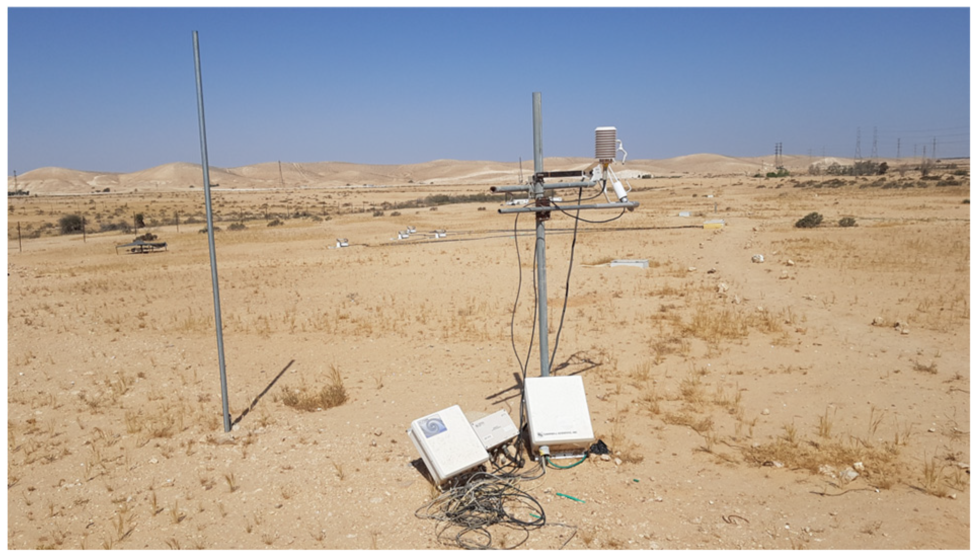
Figure 1 shows the difference between both methods.

SR analysis for estimating H assumes that a descending large parcel of air following a coherent motion remains in contact with the surface for a period (τ) during which sensible heat transfers from the surface to the parcel of air, Q (and vice versa, under stable conditions) (Figure 1). For unstable conditions, the parcel of air is warmed while remaining in contact with the surface, and its mean net temperature increase is denoted by A. By continuity (i.e., following the coherent motion), another large parcel of air sweeps into the surface, replacing the previous one and injecting sensible heat into upper air layers. Assuming continuous injections of sensible heat over half an hour, the mean H is related to the sweep–ejection frequency, 1/τ, and to the mean net amount of heat transferred from the surface into the parcel of air during τ. The net enrichment of sensible heat can be determined as Q = (ρ αZ) C_p A, where Z is the measurement height and (αZ) represents the volume per unit surface of the parcel ejected. To determine A and τ, the temperature of the air should be measured at high frequency, typically 10 Hz. Thus, in the framework of SR, the vertical velocity for the transfer of heat near the surface (w) is expressed as

$$w_{SR}={\displaystyle \frac{\alpha Z}{\tau }}$$

(4)

and the sensible heat flux is expressed as $H_{SR}=\rho C_p{w}_{SR}A$; where the parameter α is an empirical coefficient dependent on the measurement height and atmospheric stability [14,16,20,21,22,23]. The rearrangement of H_SR yields the following [16,17]:

$$H_{SR}=\rho C_p\sqrt{{\displaystyle \frac{kz{u}_{*}{{\phi }_h}^{-1}}{\pi \tau }}}A$$

(5)

ϕ_h is the stability correction function for heat transfer evaluated at z/L. Using thermal infrared imagery with a large field of view and operating at a high frequency (1 Hz–52 Hz), spatial trends in LST along transects in the wind direction were related to coherent motions [24]. Under unstable conditions, LST abruptly drops when a descending cool parcel of air reaches the ground, and after the sweep, LST gradually increases. Provided that the surface is homogeneous, the difference between the land surface temperature and the temperature of the air measured at a reference height is related to the net temperature increase for a parcel of air following a coherent motion. Assuming regular injections of sensible heat over half an hour and using the definition of mean kinematic sensible heat, the following approach was proposed:

$${\displaystyle \frac{A}{\left(LST-T\right)}}={\displaystyle \frac{w_{MOST}}{w_{SR}}}$$

(6)

where A and $\left(LST-T\right)$ both express the heat source strength and $w_{MOST}$ is the vertical velocity for the transfer of heat near the surface. It is expressed as $w_{MOST}={\displaystyle \frac{1}{r_{\mathrm{a}\mathrm{h}}}}$. The following relationship is used, involving the ramp period of a coherent motion determined at the measurement height z and the friction velocity [22]:

$${\displaystyle \frac{1}{\tau }}={\displaystyle \frac{u_{*}}{z}}\lambda$$

(7)

where $\lambda$ is an empirical coefficient. Combining Equations (6) and (7), the vertical velocity ratio is

$${\displaystyle \frac{w_{MOST}}{w_{SR}}}={\displaystyle \frac{1}{r_{\mathrm{a}\mathrm{h}}}}\left({\displaystyle \frac{1}{\alpha \lambda }}\right){\displaystyle \frac{1}{u_{*}}}$$

(8)

Stable conditions. Combining Equations (2)–(8), the sensible heat flux is

$$H_{SR-LST}=\rho C_p{\left({\displaystyle \frac{k^3}{\pi }}{\left({\displaystyle \frac{1}{{\lambda \alpha }^2 }}\right)\varphi }_h^{-1} \right)}^{1/2}{ u}_{*}\left({\displaystyle \frac{LST-T}{\mathit{ln}\left(\frac{z}{z_{0\mathrm{h}}}\right){-\mathsf{\Psi }}_h}}\right)$$

(9)

The similarity relationship is ${\varphi }_h$= $\left(1+5{\displaystyle \frac{z}{L}}\right)$ [19].

Unstable conditions. Defining the non-dimensional relationship,

$${\displaystyle \frac{1}{\lambda }}{\left({\displaystyle \frac{k}{\alpha }}\right)}^2{\left({\displaystyle \frac{kz}{z_{0h}}}\right)}^{1/3}\left({\displaystyle \frac{u_{*}}{u}}\right)=C$$

(10)

and combining Equations (9) and (10), the sensible heat flux is

$$H_{SR-LST}=\rho C_p{\left({\displaystyle \frac{k}{\pi }}{C\left({\displaystyle \frac{z_{0h}}{kz}}\right)}^{1/3}{\varphi }_h^{-1} u{ u}_{*}\right)}^{1/2}\left({\displaystyle \frac{LST-T}{\mathit{ln}\left(\frac{z}{z_{0\mathrm{h}}}\right){-\mathsf{\Psi }}_h}}\right)$$

(11)

We note that the proposal of Equation (10) was found as a result of a number of different parameter fittings. For unstable conditions the ratio ${\displaystyle \frac{w_{MOST}}{w_{SR}}}$ (Equation (8)) has to be evaluated assuming neutral conditions [25,26,27]. Thus, combining Equation (11) along with the relationship ${\varphi }_h^{-1}$ = ${\displaystyle \frac{1}{0.31}}$ ${\left(-{\displaystyle \frac{z}{L}}\right)}^{1/3}$ [28]

$$H_{SR-LST}=\rho C_p{\left({\displaystyle \frac{k}{\pi }}{\displaystyle \frac{C}{0.31}}{\left({\displaystyle \frac{g{z}_{0\mathrm{h}}}{T}}\right)}^{1/3}u\right)}^{3/5}{\left({\displaystyle \frac{LST-T}{\mathit{ln}\left(\frac{z}{z_{0\mathrm{h}}}\right)}}\right)}^{6/5}$$

(12)

Hypotheses. Regardless of the stability conditions, here, is proposed to evaluate $z_{0m}$,$z_{0h}$, $\lambda$, and $\alpha$ under neutral conditions. The corresponding values of $\lambda$ and $\alpha$ were determined, as shown in Section 3.1. Therefore, the parameter $k{B}^{-1}$ = $\mathit{ln}\left({\displaystyle \frac{z_{0m}}{z_{0h}}}\right)$ was set to 2 [29], and thus $z_{0h}=z_{0m}{e}^{-2}$. Regardless of the climate, the surface and measurement height the values of $\lambda$, $\alpha$, and the parameter C were assumed to be fairly constant.

3. Data and Methods

The H_SR-LST was tested using data collected in four experiments conducted over bare soil: the Tibetan Plateau (URL accessed 8 April 2025, https://archive.eol.ucar.edu/projects/ceop/dm/insitu/sites/ceop_ap/Tibet/Amdo-Tower/), north-eastern China (two locations, URL accessed 8 April 2025, https://archive.eol.ucar.edu/projects/ceop/dm/insitu/sites/ceop_ap/Tongyu/Grassland/ and https://archive.eol.ucar.edu/projects/ceop/dm/insitu/sites/ceop_ap/Tongyu/Cropland/), and the Negev desert, Israel (Figure 2).

The dataset has been analyzed in different international projects and a national project (see

Table 1. Experimental description.

Site: 1 Project Lat, Lon, Alt (m)	Amdo GAME-Tibet 32.2, 91.6, 4700	TY-Crop CEOP 44.4, 122.8, 184	TY-Grass CEOP 44.4, 122.8, 184	Wadi Mashash Nacional 31.13, 34.88, 400
Campaign	May–September 1998	October 2002–December 2004	October 2002–December 2004	January–August 2022
Bare surface	Up to June 15	November–March	November–March	Always
Landscape	Flat	Flat	Flat	Flat
Zom (mm)	2.2	6.10	2.24	4.50
Wind speed (m)	1.9, 6.0, 14.1	2.36, 4.36, 8.36, 12.36,	1.76, 4.36, 8.36,	2
		16.65	12.86, 17.46
Air Temp. (m)	1.55, 5.65, 13.75	1.95, 3.95, 7.95,	1.35, 3.95, 7.95,	2
		11.95, 17.36	12.45, 17.05
LST (m)	4	3	2	2
Emissivity	0.97	0.96	0.96	0.95
EC system (m)	2.85	3.5	2	2

¹ Global Energy and Water cycle Experiment (GEWEX) Asian Monsoon Experiment on the Tibetan Plateau (GAME-Tibet). Coordinated Enhanced Observing Period (CEOP).

). The sites represent a range of arid and semiarid environments, covering surface roughness lengths for momentum in the range of 2.2–6.1 mm [30] and measurement heights between 0.5 and 20 m. The $z_{om}$ was determined using the wind log-law under neutral conditions, and thus the optimal value corresponds to the peak frequency in the histogram of ln ($z_{om}$) obtained at neutral conditions (ln ($z_{om}$) = ln (z) − k u/u_*).

In the Tibetan Plateau, the station was located at Amdo (or Anduo; 32.2 Lat., 91.6 Lon., 4700 m asl), a relatively smooth and flat surface, which was bare until mid-June (pre-monsoon dry season). The wind speed and air temperature were measured using WS-51 (Ogasawara) and HMP35D (Vaisala), respectively, and LST was measured via extraction from the two longwave radiation measurements (PIR, Eppley) using an emissivity of 0.97 for the soil surface. Longwave radiation was corrected for the dome temperature. The surface was dry during the pre-monsoon period [31]. The EC system was composed of a three-dimensional sonic anemometer (DAT-300, Kaijo-Denky, Tokyo, Japan) and an infrared hygrometer (AH-300, Kaijo). The surface roughness length for the determined momentum was 2.2 mm. We note that, accounting for the stability conditions, the latter was reported as $z_{0m}$= 0.86 mm [30].

In north-eastern China, two stations were installed at Tongyu, one over corn (TY-crop; 44.4 Lat., 122.8 Lon, 184 m asl) and the other over degraded grassland (TY-grass; 44.4 Lat., 122.8 Lon., 184 m asl). The landscape was flat and the distance between stations was 5 km. The soil in both sites was bare from late fall to early spring [32]. The data for both sites were analyzed for the bare soil periods during the period 2002–2004. In both sites, wind speed and the air temperature were measured using 034A_L (Met-One) and HMP35D (Vaisala), respectively, and the longwave components of the radiation (CG4, Kipp and Zonen) were used to retrieve the land surface temperature. The EC systems were composed of a CSAT3 (Campbell Scientific Inc.) and a CS7500 (LI-COR). However, the friction velocity was not available and, therefore, the surface roughness length for momentum reported in [33] was taken as an approximation.

In the Negev desert, Israel, a measurement system was installed at the Mashash Experimental Farm (31.08 Lat., 34.53 Lon., 400 m asl) over a bare flat surface of loess soil [33]. Wind speed and air temperature were measured using 014A (Met-One) and HMP35D (Vaisala), the LST was calculated from two longwave radiation sensors (CG4; Kipp and Zonen), and the EC system was composed of a CSAT3 (Campbell Scientific Inc., North Logan, UT, USA) and a CS7500 (LI-COR). The optimum surface roughness length for momentum was 4.5 mm and the emissivity was 0.95. Even at night, the EC sensible heat flux was positive. Therefore, no stable cases were available. Additional relevant details of the experimental sites are summarized in Table 1.

3.1. Determining SR Parameters $\lambda$ and $\alpha$ and C Under Neutral Conditions

From data collected in an experiment conducted on a bare plot during 19 July–18 September, at the University of British Columbia (Plant Science Research Station in Vancouver), 1994 [22]. The air temperature was measured at z = 0.03 m with fine-wire thermocouples (chromel-constantan, 25 μm in diameter) was used to determine the $\alpha$ parameter with the measured sensible heat flux [21,22]. The $z_{om}$ was determined from mean horizontal wind speed profiles measured using custom-made miniature hot-wire anemometers. The plot was non-irrigated and the fetch was considered unlimited (25 × 25 m² fetch). The measurements were made for nearly neutral conditions (dawn (0600–0700 PST) and dusk (1700–1800 PST)) simultaneously at four different heights, at z = 4, 7, 10, and 13 cm above the bare soil. They were used to estimate $z_{om}$ using the standard technique of fitting to the logarithmic law. The reported optimal value for $z_{om}$ determined at neutral conditions was $z_{om}$ = 0.005 m. With the $u_{*}$ (obtained from the wind log-law), the coeficient $\lambda$ was determined. The mean values of $\alpha$ and $\lambda$ (both determined at z = 0.03 m) were 0.684 and 0.398, respectively [22]. Under neutral conditions, $z_{0h}=z_{0m}{e}^{-2}$, and therefore the C value, was 0.5. Provided that the mean values of $\alpha$ and $\lambda$ were the same, and assuming surfaces with $z_{om}$ ranged between 0.001 m and 0.007 m, the maximum C value differed by 10% (with respect to 0.5). We note that the value ${\displaystyle \frac{1}{\lambda }} {\left({\displaystyle \frac{k}{\alpha }}\right)}^2$ plays a role in Equation (10). For bare soil the latter was 0.86. However, it appears rather robust given that, in other contexts such as in Douglas fir forests (16.7 m tall and Z was 23 m), it was 0.85 [22].

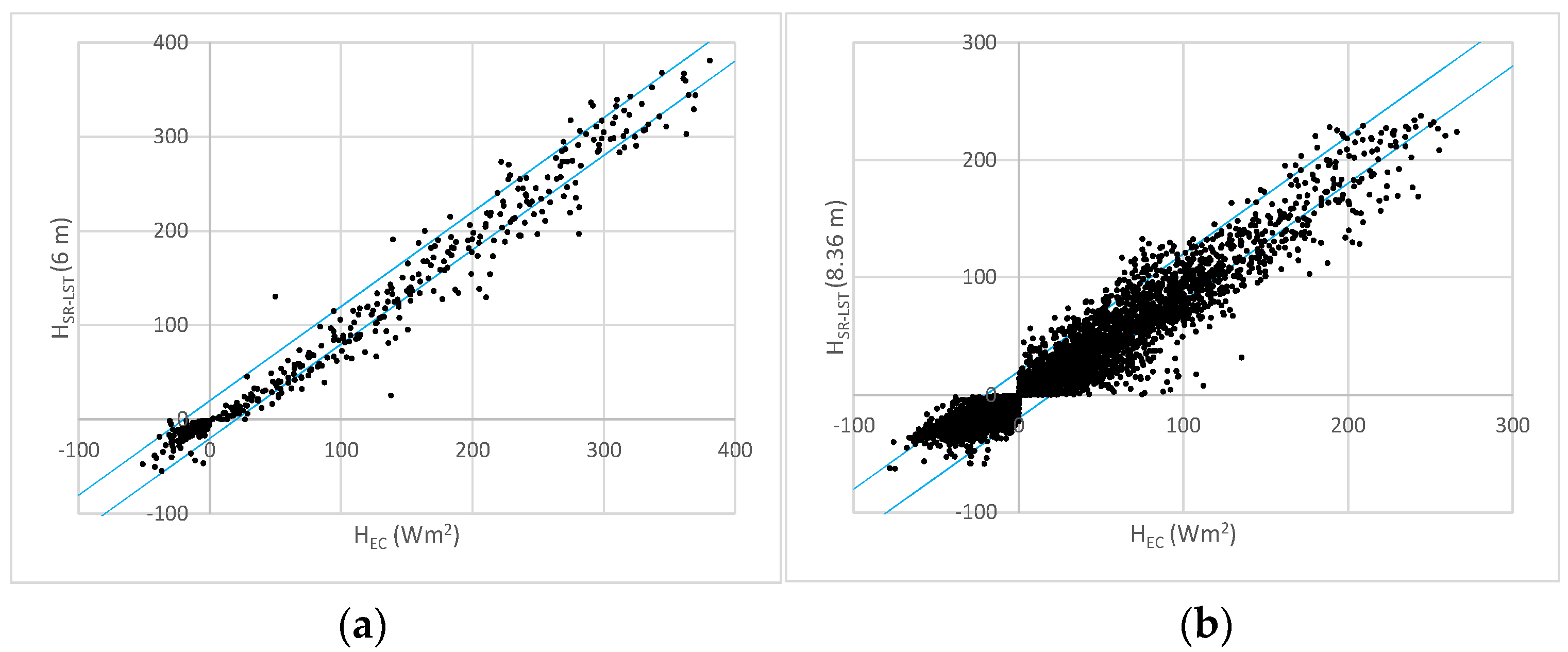
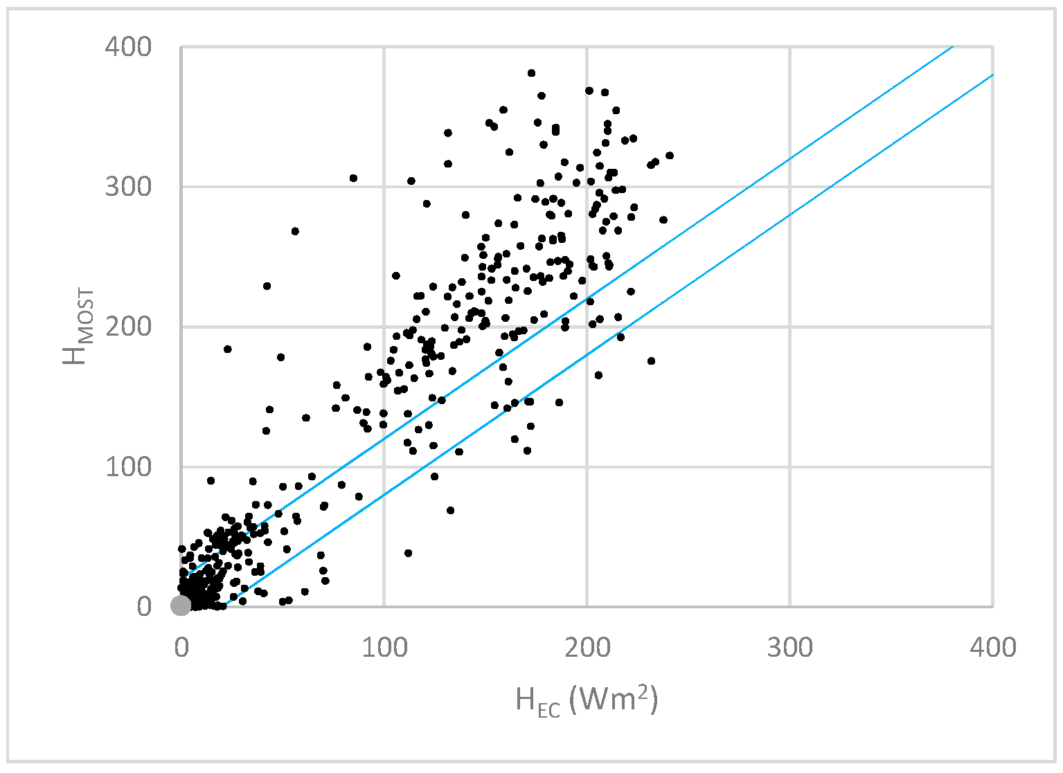
3.2. Estimating the Sensible Heat Flux. Comparison and Evaluation

For MOST, the sensible heat flux was estimated iteratively because the equations converged. Starting at neutral conditions, the first approximation of $H_{MOST}$ was estimated from the wind log-law. Next, the stability parameter was calculated, so the second approximation of $H_{MOST}$ was calculated and so on. A similar procedure was applied to determine $H_{SR-LST}$ under stable conditions. For unstable cases, $H_{SR-LST}$ determination is direct.

Uncertainties in the measurement of the actual sensible heat flux were taken into account. Therefore, as a rule of thumb, the comparison was made for samples accomplishing that error in the surface energy balance closure, which was less than 150 Wm² (R_n–G–LE_EC–H_EC $\le$150 Wm², where R_n, G and LE_EC are the net radiation, the soil heat flux, and the EC latent heat flux, respectively); the wind speed measured at the lowest level was u $\ge$0.5 m/s (to ensure turbulent mixing), and the signs of (LST–T) and H_EC were the same.

The results of the linear regression analysis (a and b denoting the slope and the intercept in Wm⁻², respectively), the coefficient of determination (R²), the root mean square error (RMSE in Wm⁻²) and the RMSE over the mean H_EC, E $(\mathrm{R}\mathrm{M}\mathrm{S}\mathrm{E}/\overline{H_{EC}}$ expressed in %), comparing H_SR-LST and H_MOST against H_EC, were used to evaluate performance. Given the inherent 10% variability in the surface boundary layer [18], an E value of up to 15% is expected. Accounting for other potential errors, uncertainties of measurements, and calculating the reference [34,35], as rule of the thumb, E values of up to 25%, 30% and 40% were considered excellent, good, and tolerable, respectively. The accuracy of the CSAT3 in measuring the sensible heat flux is ±20 Wm⁻² [34,36,37,38]. The intercepts below the latter threshold were considered negligible.

4. Results and Discussion

Figure 3 compares the performance of H_SR-LST at two sites, Ambo and TY- grass, showing the range of the sensible heat flux at these sites.

4.1. Stable Cases

Table 2. Comparing H_SR-LST and H_MOST against H_EC for different measurement heights and sites. Setting $k{B}^{-1}$ = 2. H is the measurement height, a is the slope, and b is the intersect (Wm⁻²), RMSE in Wm⁻² and N represent the available data.

Method:		HSR-LST					HMOST
H (m)	N:	a	b	R2	RMSE	E (%)	a	b	R2	RMSE	E (%)
Amdo	177
1.95		0.78	−3	0.58	8	63	1.08	−3	0.53	11	81
6		0.76	−2	0.53	8	57	1.14	−1	0.55	11	72
14.1		0.70	−1	0.53	8	56	1.11	1	0.53	10	65
TY-grass	4401
1.76		0.49	−8	0.42	10	61	0.60	−11	0.40	12	70
4.36		0.46	−8	0.45	10	58	0.64	−10	0.47	11	60
8.36		0.46	−7	0.51	10	58	0.68	−7	0.54	9	50
12.86		0.41	−5	0.51	11	62	0.63	−5	0.53	10	47
17.46		0.40	−5	0.54	11	63	0.62	−4	0.54	10	48
TY-crop	2985
2.36		0.84	−8	0.63	11	59	1.05	−11	0.62	16	81
4.36		0.76	−6	0.62	9	48	0.99	−7	0.58	13	62
8.36		0.63	−4	0.62	9	47	0.86	−3	0.52	11	47
12.36		0.57	−3	0.61	10	53	0.77	−2	0.44	13	52
17.05		0.51	−2	0.62	12	58	0.69	−1	0.40	10	39

shows the results obtained for Ambo, TY-grass, and TY-crop. The intercepts were considered small, ranging between −11 Wm⁻² and 1 Wm⁻². Regardless of the site, the slopes from H_SR-LST were lower than 1 (0.84 ≤ a ≤ 0.40), and they were consistently lower compared to height. So, H_SR-LST was z-dependent. The slopes from H_MOST ranged between 1.14 and 0.60. When the slopes were calculated through the origin, they were z-dependent (i.e., consistently lower compared to height). The range was 0.72 ≤ a ≤ 1.40. Assuming that the H_EC was correct, this issue appears to be related to the modelling itself, such as the estimation of friction velocity. The coefficients of determination obtained using H_SR-LST (0.42 ≤ a ≤ 0.63) and H_MOST (0.40 ≤ a ≤ 0.62) were, in practice, the same. The RMSE values were similar, being slightly lower for H_SR-LST (8 Wm⁻² ≤ RMSE ≤ 12 Wm⁻²) than for H_MOST (9 Wm⁻² ≤ RMSE ≤ 16 Wm⁻²). The RMSE values were considered, in practice, constant and, in any case, were not z-dependent. Either for H_SR-LST and H_MOST, the E values were intolerable (Table 2). However, given the low values of the H_EC, the best statistics for comparison were the R² and the RMSE. Thus, considering the RMSE, H_SR-LST was slightly better than H_MOST. Despite the underestimation, the statistic R² was distorted by a few samples. For instance, after filtering three samples (over 177 in total), as shown in Figure 3a (for stable cases), the performance improved with the following results: a = 0.81, b = −1 Wm², R² = 0.67, RMSE = 6 Wm², and E = 45%.

4.2. Unstable Cases

Table 3. Comparing H_SR-LST and H_MOST against H_EC for different measurement heights and sites. Setting $k{B}^{-1}$ = 2. H is the measurement height, a is the slope, b is the intersect (Wm⁻²), RMSE in Wm⁻² and N are the available data.

Method:		HSR-LST					HMOST
H (m)	N:	a	b	R2	RMSE	E (%)	a	b	R2	RMSE	E (%)
Amdo	312
1.95		1.04	−15	0.96	23	15	1.26	−12	0.93	53	33
6		1.01	−14	0.96	25	15	1.26	−12	0.93	53	33
14.1		0.97	−11	0.95	28	17	1.25	−10	0.93	51	32
TY-grass	2744
1.76		0.93	−2	0.83	23	38	1.18	3	0.85	31	50
4.36		0.89	0	0.86	20	34	1.15	4	0.87	27	46
8.36		0.88	0	0.87	20	34	1.15	3	0.88	26	44
12.86		0.86	1	0.87	19	33	1.14	4	0.88	25	44
17.46		0.85	1	0.87	20	34	1.13	3	0.88	24	42
TY-crop	2386
2.36		1.27	−13	0.89	33	40	1.51	−10	0.87	56	68
4.36		1.24	−12	0.89	31	38	1.47	−9	0.88	52	64
8.36		1.20	−7	0.88	30	37	1.44	−5	0.88	52	64
12.36		1.17	−8	0.89	27	33	1.42	−7	0.88	48	60
17.05		1.12	−6	0.89	25	32	1.38	−5	0.89	45	58
Wadi M.	1782
2		1.10	−9	0.78	51	39	1.25	−5	0.76	69	56
Morning	470	1.04	−10	0.66	50	44	1.21	−8	0.63	69	64
Noon	768	1.17	−19	0.70	64	34	1.26	26	0.45	133	70
Afternoon	464	1.11	1	0.89	33	40	1.37	6	0.86	62	78

shows the results obtained for the Ambo, TY-grass, TY-crop and Wadi Mashash sites. The intercepts obtained ranged between -15 Wm² and 4 Wm². The performance for H_SR-LST at Ambo was excellent (Figure 3a for unstable cases), the slopes and the coefficients of determination were close to 1, 0.97 ≤ a ≤ 1.04 and 0.95 ≤ R² ≤ 0.96, respectively, and the E values had a range of 14% ≤ E ≤ 17%. These results were the best (Table 3), partly because Ambo was windy (minimum and the average wind speeds measured at 2 m were 0.7 m/s and 5.7 m/s, respectively) and, therefore, the mechanical turbulence predominated. The latter reinforces the best SR performance at high wind speeds [27,39]. The slopes obtained at TY were lower than 1 at TY-grass (0.85 ≤ a ≤ 0.93) and greater than 1 for TY-crop (1.12 ≤ a ≤ 1.27). The coefficients of determination were good, ranging between 0.83 and 0.89 at TY. In general, Table 3 shows that the E values were slightly smaller at TY-grass (33% ≤ E ≤ 38%) than at TY-crop (32% ≤ E ≤ 40%). The wind speed was similar at both sites (minimum and the average wind speeds at 1.95 m were 0.5 and 0.55 m/s and 4.6 m/s and 4.7 m/s at TY-grass and TY-crop, respectively). Likely, the difference with the slopes obtained at TY-grass and TY-crop may not be wind-speed-related. Perhaps, the z_0m (reported in Table 1) was different to the corresponding values at neutral conditions. Regardless of potential uncertainties, the performance was tolerable at TY sites. At Wadi Mashash, the slope was slightly greater than 1, thus, on average, H_SR-LST overestimated H_EC by the 1.06 (determined using linear regression forced though the origin). The coefficient of determination was 0.78 and the E value was 39%, so the performance was tolerable (Table 3). To analyze the latter correlation, the dataset was split into three sub-datasets called morning (from sunrise to 11.00 h), noon (11.30 h up to 14.00 h), and afternoon (14.30 h to sunset), representing the different size of coherent structures and stability conditions. Using linear regression forced through the origin, on average, H_SR-LST was 0.97, 1.08 and 1.10 times the H_EC. The coefficients of determination were 0.66, 0.70, and 0.87, the E values were 44%, 34%, and 40% (Table 3) and Figure 4 show the Bland–Altman plots for the morning, noon, and afternoon, respectively. Perhaps the reference taken underestimated the actual sensible heat flux, especially around noon in the summer, when the biggest size of the thermal coherent structures predominated. The latter explains the tendency of SR to overestimate EC [39,40,41,42,43,44]. A few samples were able to distort the statistics in Figure 4. For instance, after filtering 29 samples (corresponding to the ±1.96 standard deviation; over 464 in total) in the afternoon subset, the performance was excellent; a = 1.09, b = −1 Wm², R² = 0.95, RMSE = 22 Wm², and E = 28%. All the samples that distorted the statistics (Figure 4c) were taken during the period ranging between 15.00 h and 16.00 h; most of them were gathered in summer. However, in principle, the data filtered should not treated as outliers (there are too many unknowns related to the estimation of the actual H).

Regardless of the site and the measurement height, the correlations obtained by MOST were similar to SR. However, H_MOST overestimated H_EC, leading to the slopes ranging in the interval 1.13 ≤ a ≤ 1.51, and the E values were, in general, intolerable (32% ≤ E ≤ 68%). H_MOST was tolerable at Amdo, however, never superior to H_SR-LST. Given the good correlation obtained by MOST, H_MOST improved when using the site-specific values of $k{B}^{-1}$. When using $k{B}^{-1}$ values of 2.36, 4.49, 3.64 at Amdo, TY-crop, and TY-grass, respectively, H_MOST performed well, yielding slopes close to one and intercepts close to zero [30]. This issue was also observed at Wadi Mashash, requiring a $k{B}^{-1}$ of around 5 to achieve a performance similar to H_SR-LST. Figure 5 shows the H_MOST performance in the afternoon using $k{B}^{-1}$ = 2. Using $k{B}^{-1}$ = 4.9, the slope, intercept, and R² values were 1.00, 5 Wm⁻², and 0.85, respectively, and E was 38%.

Finally, further research is required to evaluate the H_SR-LST for different climates to explore its performance over the glove, especially in the summer season.

5. Conclusions

The key for estimating the sensible heat flux combining SR and MOST concepts was to set the parameter $k{B}^{-1}$ as a constant ($k{B}^{-1}$ = 2 valid at neutral conditions). For stable conditions, the performances of H_SR-LST and H_MOST were similar and both were considered unacceptable (E > 40%). However, in terms of the root mean square error, the H_SR-LST performance was slightly better than H_MOST. The former’s RMSE ranged between 8 Wm⁻² and 12 Wm⁻² and the latter between 9 Wm⁻² and 16 Wm⁻². For unstable conditions, the key was to implement a non-dimensional invariant parameter. H_SR-LST performed, in general, rather close to the EC method ($15\%\le$ E $\le$ 40%) while H_MOST required site-specific calibration of $k{B}^{-1}$. The local meteorological features and soil conditions had a minor impact on H_SR-LST than on H_MOST. The latter is important for practical implications of H SR-LST for climate change studies or water resource management in drylands. It was concluded that H_SR-LST was, at least, comparable to H_MOST for stable conditions and was more suitable for unstable conditions because it was exempt from calibration.

References

1. Schmid, P.; Niyogi, D. A method for estimating planetary boundary layer heights and its application over the ARM Southern Great Plains site. J. Atmos. Ocean. Technol. 2012, 29, 316–322. [Google Scholar] [CrossRef]
2. Compton, J.C.; Delgado, R.; Berkoff, T.A.; Hoff, R.M. Determination of planetary boundary layer height on short spatial and temporal scales: A demonstration of the covariance wavelet transform in ground-based wind profiler and lidar measurements. J. Atmos. Ocean. Technol. 2013, 30, 1566–1575. [Google Scholar] [CrossRef]
3. Brunet, Y. Turbulent flow in plant canopies: Historical perspective and overview. Bound-Layer Meteorol. 2020, 177, 315–364. [Google Scholar] [CrossRef]
4. Kustas, W.P.; Blanford, J.H.; Stannard, D.I.; Daughtry, C.S.T.; Nichols, W.D.; Weltz, M.A. Local energy flux estimates for unstable conditions using variance data in semiarid rangelands. Water Resour. Res. 1994, 30, 1351–1361. [Google Scholar] [CrossRef]
5. Drexler, J.Z.; Snyder, R.L.; Spano, D.; Paw, U.K.T. A review of models and micrometeorological methods used to estimate wetland evapotranspiration. Hydrol. Process. 2004, 18, 2071–2101. [Google Scholar] [CrossRef]
6. Pozníková, G.; Fischer, M.; van Kesteren, B.; Orság, M.; Hlavinka, P.; Žalud, Z.; Trnka, M. Quantifying turbulent energy fluxes and evapotranspiration in agricultural field conditions: A comparison of micrometeorological methods. Agric. Water Manag. 2018, 209, 249–263. [Google Scholar] [CrossRef]
7. Verhoef, A.; Mcnaughton, K.G.; Jacobs, A.F.G. A parameterization of momentum roughness length and displacement height for a wide range of canopy densities. Hydrol. Earth Syst. Sci. Discuss. 1997, 1, 81–91. [Google Scholar] [CrossRef]
8. Timmermans, W.J.; Kustas, W.P.; Anderson, M.C.; French, A.N. An intercomparison of the Surface Energy Balance Algorithm for Land (SEBAL) and the Two-Source Energy Balance (TSEB) modeling schemes. Remote Sens. Environ. 2007, 108, 369–384. [Google Scholar] [CrossRef]
9. Sun, S.K.; Li, C.; Wang, Y.B.; Zhao, X.N.; Wu, P.T. Evaluation of the mechanisms and performances of major satellite-based evapotranspiration models in Northwest China. Agric. For. Meteorol. 2020, 291, 108056. [Google Scholar] [CrossRef]
10. Anderson, M.C.; Kustas, W.P.; Norman, J.M.; Diak, G.T.; Hain, C.R.; Gao, F.; Yang, Y.; Knipper, K.R.; Xue, J.; Yang, Y.; et al. A brief history of the thermal IR-based Two-Source Energy Balance (TSEB) model—Diagnosing evapotranspiration from plant to global scales. Agric. For. Meteorol. 2024, 350, 109951. [Google Scholar] [CrossRef]
11. Norman, J.M.; Kustas, W.P.; Humes, K.S. Source approach for estimating soil and vegetation energy fluxes in observations of directional radiometric surface temperature. Agric. For. Meteorol. 1995, 77, 263–293. [Google Scholar] [CrossRef]
12. Sánchez, J.M.; López-Urrea, R.; Valentín, F.; Caselles, V.; Galve, J.M. Lysimeter assessment of the Simplified Two-Source Energy Balance model and eddy covariance system to estimate vineyard evapotranspiration. Agric. For. Meteorol. 2019, 274, 172–183. [Google Scholar] [CrossRef]
13. Castellví, F.; González-Dugo, M.P. A one–source model to estimate sensible heat flux in agricultural landscapes. Agric. For. Meteorol. 2021, 310, 108628. [Google Scholar] [CrossRef]
14. Paw, U.K.T.; Qiu, J.; Su, H.B.; Watanabe, T.; Brunet, Y. Surface renewal analysis: A new method to obtain scalar fluxes without velocity data. Agric. For. Meteorol. 1995, 74, 119–137. [Google Scholar] [CrossRef]
15. Raupach, M.R.; Finnigan, J.J.; Brunet, Y. Coherent eddies in vegetation canopies: The mixing-layer analogy. Bound-Layer Meteorol. 1996, 78, 351–382. [Google Scholar] [CrossRef]
16. Castellví, F. Combining surface renewal analysis and similarity theory: A new approach for estimating sensible heat flux. Water Resour. Res. 2004, 40, W05201. [Google Scholar] [CrossRef]
17. Fisher, M.; Katul, G.G.; Noormets, A.; Poznikova, G.; Domec, J.C.; Orság, M.; Zalud, Z.; Trnka, M.; King, J.S. Merging flux-variance with surface renewal methods in the roughness sublayer and the atmospheric surface layer. Agric. For. Meteorol. 2023, 342, 109692. [Google Scholar] [CrossRef]
18. Brutsaert, W.H. Evaporation into the Atmosphere. Environmental Fluid Mechanics, 1st ed.; Kluwer Academic Publishers: Dordrecht, Switzerland; Boston, MA, USA; London, UK, 1982; pp. 1–400. [Google Scholar]
19. Dyer, A.J. A review of flux-profile relationships. Bound-Layer Meteorol. 1974, 7, 363–372. [Google Scholar] [CrossRef]
20. Katul, G.G.; Hsieh, C.I.; Oren, R.; Ellsworth, D.; Philips, N. Latent and sensible heat flux predictions from a uniform pine forest using surface renewal and flux variance methods. Bound-Layer Meteorol. 1996, 80, 249–282. [Google Scholar] [CrossRef]
21. Chen, W.; Novak, M.D.; Black, T.A.; Lee, X. Coherent eddies and temperature structure functions for three contrasting surfaces. Part I. Ramp model with finite micro-front time. Bound-Layer Meteorol. 1997, 84, 99–123. [Google Scholar] [CrossRef]
22. Chen, W.; Novak, M.D.; Black, T.A.; Lee, X. Coherent eddies and temperature structure functions for three contrasting surfaces. Part II. Renewal model for sensible heat flux. Bound-Layer Meteorol. 1997, 84, 125–147. [Google Scholar] [CrossRef]
23. Haymann, N.; Lukyanov, V.; Tanny, J. Effects of variable fetch and footprint on surface renewal measurements of sensible and latent heat fluxes in cotton. Agric. For. Meteorol. 2019, 268, 63–73. [Google Scholar] [CrossRef]
24. Garai, A.; Kleissl, J. Air and surface temperature coupling in the convective atmospheric boundary layer. J. Atmos. Sci. 2011, 68, 2945–2954. [Google Scholar] [CrossRef]
25. Castellví, F.; Gavilan, P.; Gonzalez-Dugo, M.P. Combining the bulk transfer formulation and surface renewal analysis for estimating the sensible heat flux without involving the parameter kB−1. Water Resour. Res. 2014, 50, 8179–8190. [Google Scholar] [CrossRef]
26. Castellví, F.; Cammalleri, C.; Ciraolo, G.; Maltese, A.; Rossi, F. Daytime sensible heat flux estimation over heterogeneous surfaces using multitemporal land-surface temperature observations. Water Resour. Res. 2016, 52, 3457–3476. [Google Scholar] [CrossRef]
27. Castellví, F.; Oliphant, A.J. Daytime sensible and latent heat flux estimates for a mountain meadow using in-situ slow-response measurements. Agric. For. Meteorol. 2017, 236, 135–144. [Google Scholar] [CrossRef]
28. Grachev, A.; Fairall, C.; Bradley, E. Convective Profile Constants Revisited. Bound-Layer Meteorol. 2000, 94, 495–515. [Google Scholar] [CrossRef]
29. Crago, R.D.; Qualls, R.J. Use of land surface temperature to estimate surface energy fluxes: Contributions of Wilfried Brutsaert and collaborators. Water Resour. Res. 2014, 50, 3396–3408. [Google Scholar] [CrossRef]
30. Yang, K.; Koike, T.; Ishikawa, H.; Kim, J.; Li, X.; Liu, H.; Liu, S.; Ma, Y.; Wang, J. Turbulent Flux Transfer over Bare-Soil Surfaces: Characteristics and Parameterization. J. Appl. Meteorol. Climatol. 2008, 47, 276–290. [Google Scholar] [CrossRef]
31. Tanaka, K.; Ishikawa, H.; Hayashi, T.; Tamagawa, I.; Ma, Y. Surface energy budget at Amdo on Tibetan Plateau using GAME/Tibet IOP98 data. J. Meteor. Soc. Jpn. 2001, 79, 505–517. [Google Scholar] [CrossRef]
32. Yan, X.; Yang, H.; Liu, F. Modeling of surface flux in Tongyu using the Simple Biosphere Model (SiB2). J. For. Res. 2010, 21, 183–188. [Google Scholar] [CrossRef]
33. Agam, N.; Berliner, P.R. Diurnal Water Content Changes in the Bare Soil of a Coastal Desert. J. Hydromet. 2004, 5, 922–933. [Google Scholar] [CrossRef]
34. Mauder, M.; Liebethal, C.; Göckede, M.; Leps, J.P.; Beyrich, F.; Foken, T. Processing and quality control of flux data during LITFASS-2003. Bound-Layer Meteorol. 2006, 121, 67–88. [Google Scholar] [CrossRef]
35. Frank, J.M.; Massman, W.J.; Ewers, B.E. Underestimates of sensible heat flux due to vertical velocity measurement errors in non-orthogonal sonic anemometers. Agric. For. Meteorol. 2013, 171, 72–81. [Google Scholar] [CrossRef]
36. Mauder, M.; Oncley, S.P.; Vogt, R.; Weidinger, T.; Ribeiro, L.; Bernhofer, C.; Foken, T.; Kohsiek, W.; de Bruin, H.A.R.; Liu, H. The Energy Balance Experiment EBEX-2000. Part II: Intercomparison of eddy-covariance sensors and post-field data processing methods. Bound-Layer Meteorol. 2007, 123, 29–54. [Google Scholar] [CrossRef]
37. Foken, T. Micrometeorology, 1st ed.; Springer: Berlin/Heidelberg, Germany, 2008; pp. 1–306. [Google Scholar]
38. Foken, T.; Oncley, S.P. Results of the workshop ‘Instrumental and methodical problems of land surface flux measurements’. Bull. Amer. Meteorol. Soc. 2005, 76, 1191–1193. [Google Scholar] [CrossRef]
39. Castellví, F.; Snyder, R.L.; Baldocchi, D.D. Surface energy-balance closure over rangeland grass using the eddy covariance method and surface renewal analysis. Agric. For. Meteorol. 2008, 148, 1147–1160. [Google Scholar] [CrossRef]
40. Horst, T.W.; Semmer, S.R.; Maclean, G. Correction of a Non-orthogonal, Three-Component Sonic Anemometer for Flow Distortion by Transducer Shadowing. Bound-Layer Meteorol. 2015, 155, 371–395. [Google Scholar] [CrossRef]
41. Frank, J.M.; Massman, W.J.; Swiatek, E.; Zimmerman, H.A.; Ewers, B.E. All Sonic Anemometers Need to Correct for Transducer and Structural Shadowing in Their Velocity Measurements. J. Atmos. Ocean. Technol. 2016, 33, 149–167. [Google Scholar] [CrossRef]
42. Frank, J.M.; Massman, W.J.; Stephen, C.W.; Nowicki, K.; Rafkin, S.C.R. Coordinate Rotation–Amplification in the Uncertainty and Bias in Non-orthogonal Sonic Anemometer Vertical Wind Speeds. Bound-Layer Meteorol. 2020, 175, 203–235. [Google Scholar] [CrossRef]
43. Mauder, M.; Eggert, M.; Gutsmuths, C.; Oertel, S.; Wilhelm, P.; Voelksch, I.; Wanner, L.; Tambke, J.; Bogoev, I. Comparison of turbulence measurements by a CSAT3B sonic anemometer and a high-resolution bistatic Doppler lidar. Atmos. Meas. Tech. 2020, 13, 969–983. [Google Scholar] [CrossRef]
44. Qi, Y.; Xiaodong, S.; Chen, G.; Gao, Z.; Bi, X.; Yu, L.; Mao, H. Re-estimation of the vertical sensible heat flux by determining the environmental temperature on a single-point tower measurement. Front. Earth Sci. 2024, 12, 1269252. [Google Scholar] [CrossRef]
Figure 1. Scheme for an unstable case. (a) From a Eulerian point of view, MOST assumes that the thermal mixing of the air is driven by the half-hourly wind speed measured at height, Z, and the difference between the temperatures observed at the surface, LST, and at the measurement height, T, (LST − T). The kinematic sensible heat flux is as follows: w M O S T ( L S T T ) , where w M O S T is the vertical velocity for the transfer of heat near the surface (i.e., the inverse of the aerodynamic resistance, r a h ). (b) From a Lagrangian point of view, SR analysis focuses on the role of a coherent structure (CS) through the determination of the ramp period ( τ CS) and amplitude (ACS). After a quiescent period (q), the macro-parcel of air (red) is heated for a period (l) until, by continuity, it is replaced for a period (f) by a cooler parcel (blue) coming from above with a mean temperature Tb, representing the signature of the CS (thin solid line). The kinematic sensible heat flux is as follows: w S R A , where w S R is the vertical velocity and w S R = α Z τ , with ( α Z ) being the volume of the macro-parcel of air.
Atmosphere 16 00458 g001
Figure 2. The meteorological station in Wadi Mashash.
Atmosphere 16 00458 g002
Figure 3. HSR-LST versus HEC at (a) Ambo (6 m) and (b) TY-grass (8.36 m). The blue lines represent the CSAT3 accuracy (±20 Wm−2).
Atmosphere 16 00458 g003
Figure 4. Bland–Altman plots for (a) morning, (b) noon, and (c) afternoon. SD is the standard deviation.
Atmosphere 16 00458 g004
Figure 5. HMOST versus HEC for the afternoon using k B 1 = 2. The blue lines represent the CSAT3 accuracy (±20 Wm−2).
Atmosphere 16 00458 g005