
Spatial Modeling of Trace Element Concentrations in PM10 Using Generalized Additive Models (GAMs)
 , , , , ,
  and
and
Abstract
:1. Introduction
2. Materials and Methods
2.1. Study Area
2.2. Sampling and Analysis
- Two sites (RI, MA) situated near the waste treatment power plant in the western part of the city;
- Three sites (GI, CR, HG) located near the railway in the northwest of the city;
- Six sites (CZ, HV, SA, UC, CA, CO) encompassing the busiest streets in the city center;
- Two sites representing industrial biomass heating (FA and CB, corresponding to carpentry and craftsmanship laboratories) in the southwest of the city;
- Six sites (FR, BR, AR, PI, PV, LG) designated for domestic biomass heating in townhouses located in the northern and southern regions of the city;
- Four sites (RO, OB, PR, CP) surrounding the extensive steel plant to the east of the city.

2.3. Potential Spatial Explanatory Variables
- Land use, calculated in the domain of interest at a spatial resolution of 10 m:
- Continuous urban fabric representative of continuous areas with high urban fabric (>80% coverage);
- Discontinuous urban fabric represented area with varying urban fabric densities: dense (50–80%), medium (30–50%), low (10–30%), and very low (<10%);
- Industrial commercial public representative of industrial, commercial, and public areas;
- Imperviousness, which was representative of impervious surfaces.
- 2.
- Urban morphology:
- Building heights were extracted from the Urban Atlas 2018 section of the CLMS, weighted for the corresponding urban fabric area.
- Road lengths and distances were assessed for main, secondary, tertiary, and local roads, as well as proximity to railways, utilizing Open Street Map layers (https://www.openstreetmap.org; accessed on 1 January 2024).
- Further street configuration variables were included from Urban Atlas 2018, distinguishing between fast transit roads and other roads with associated land.
- Cold and hot areas, along with scrapyard, were identified as primary point sources associated with the Terni steel plant, represented by the minimum distance from each sampling site.
- 3.
- Population:
- The number of inhabitants in 2018 was referenced from the most recent ISTAT census sections of 2011 (https://www.istat.it/it/archivio/104317; accessed on 1 January 2024).
- 4.
- Normalized Vegetation Index (NDVI):
- NDVI was included as a predictor variable, given that it serves as a better proxy for vegetation density compared to Corine Land Cover categories (urban green, natural areas). Daily updates were provided at a spatial resolution of 10 m × 10 m.
2.4. Potential Temporal Explanatory Variables—Meteorological Parameters
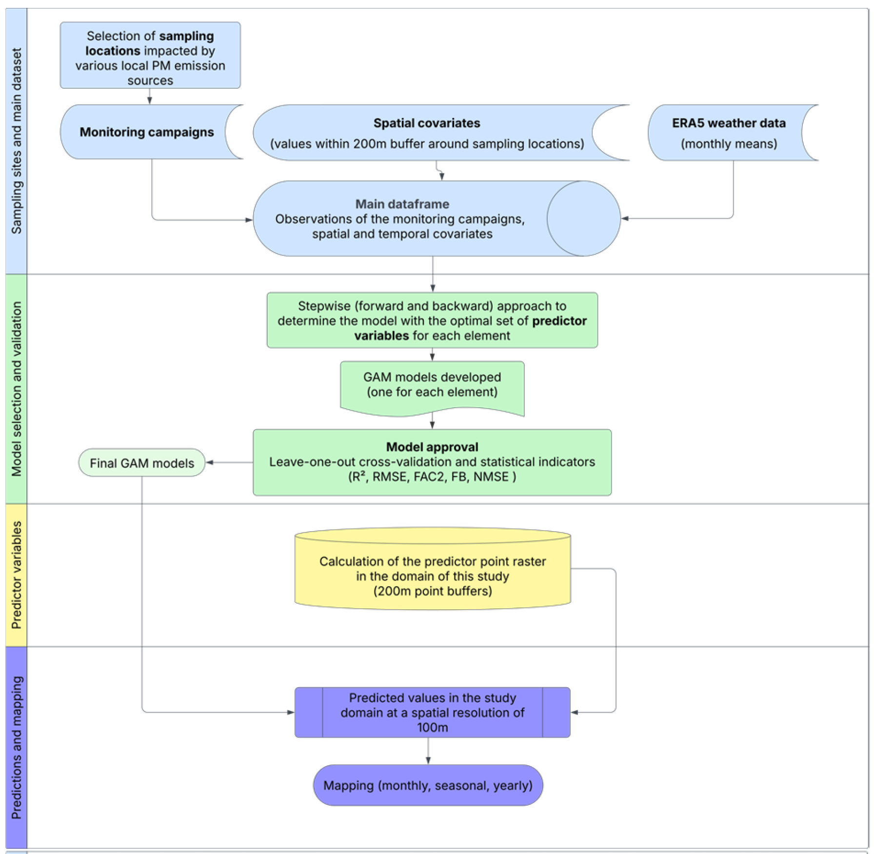
2.5. Generalized Additive Model Development
3. Results and Discussion
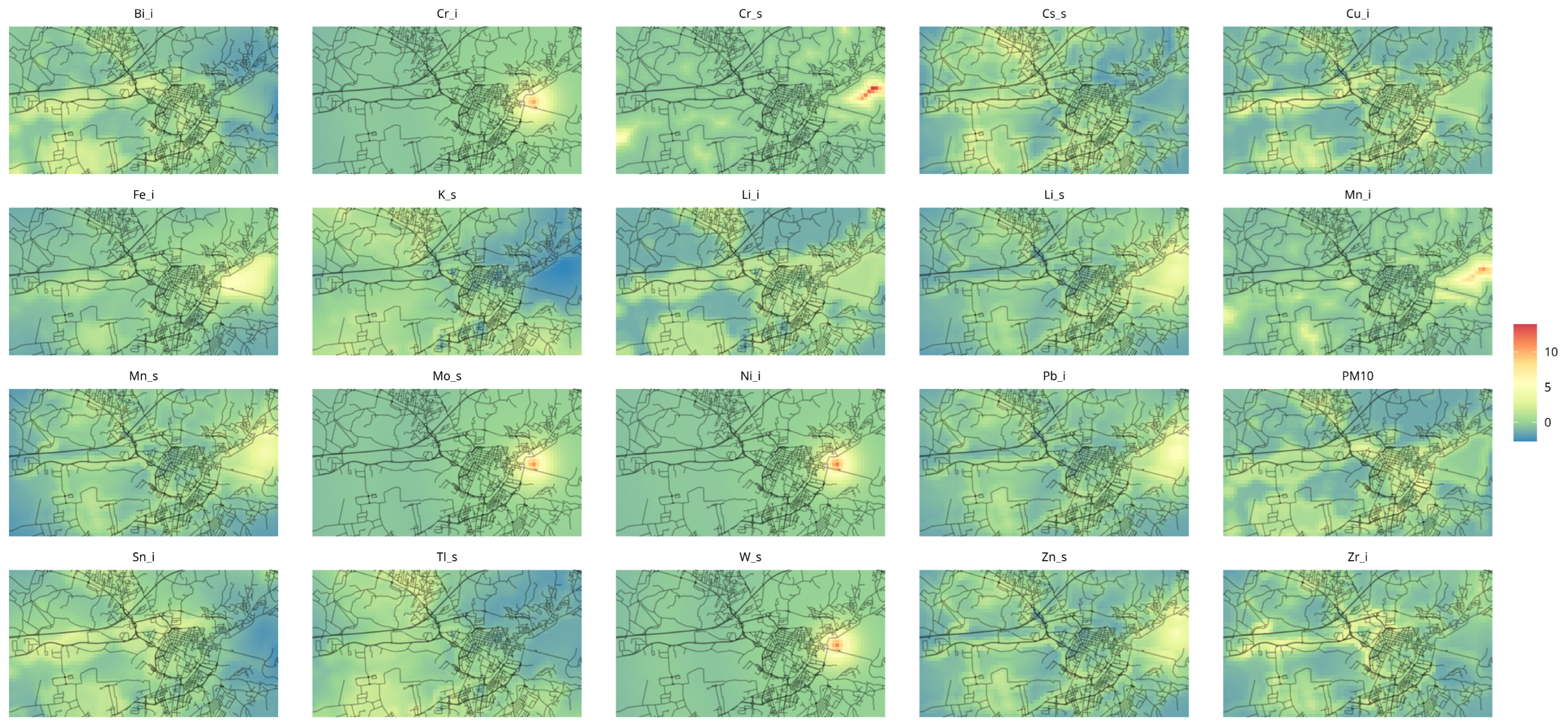
3.1. Spatial Distribution
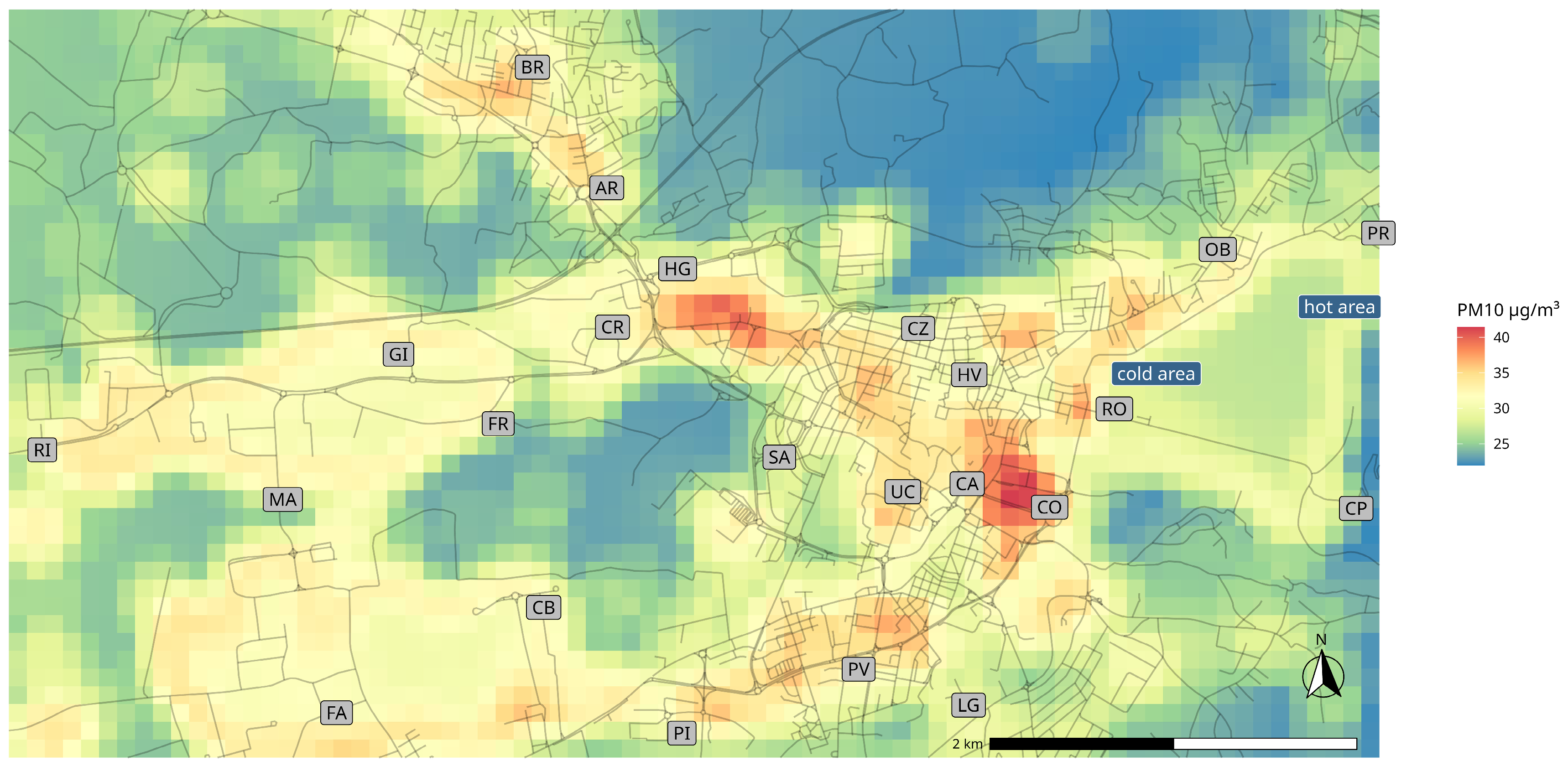
3.1.1. PM10
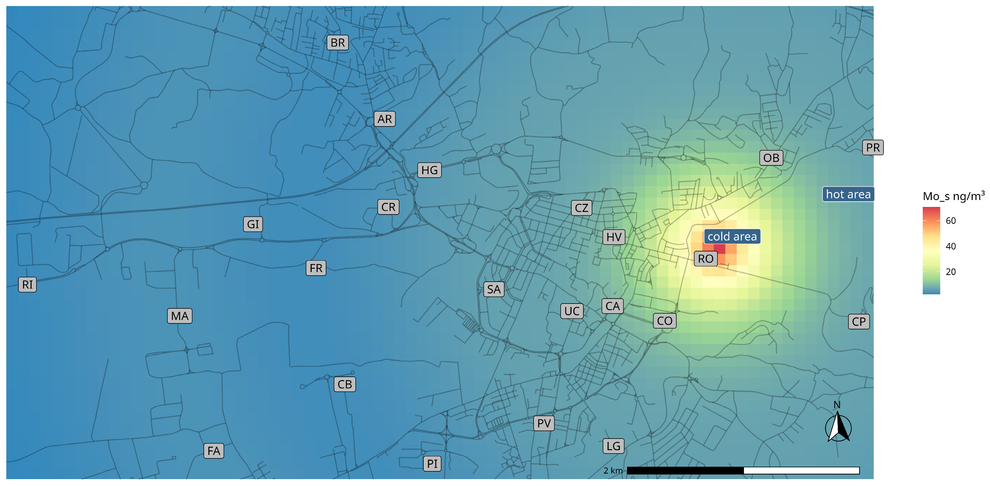
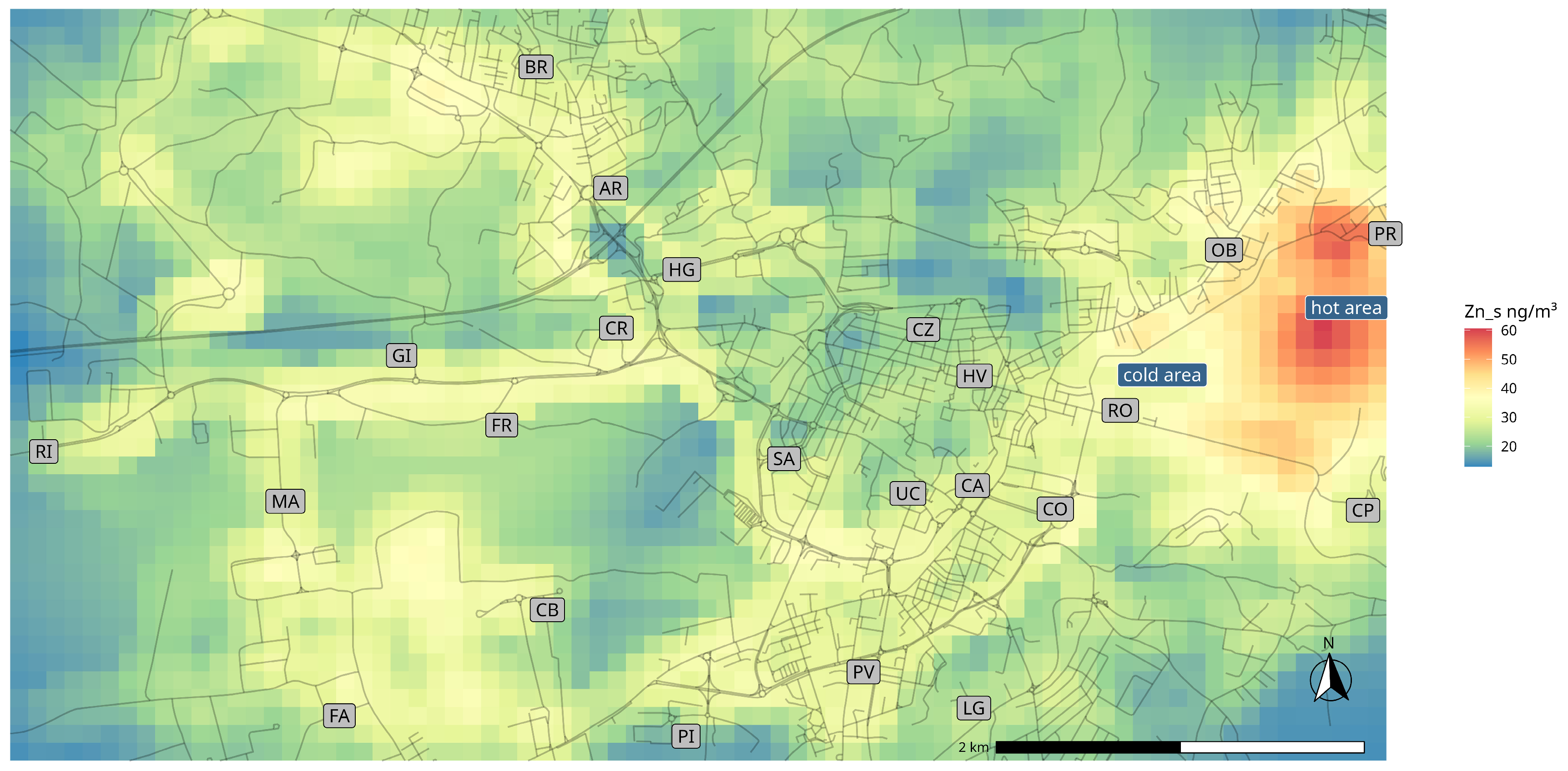
3.1.2. Steel Plant
3.1.3. Biomass Heating
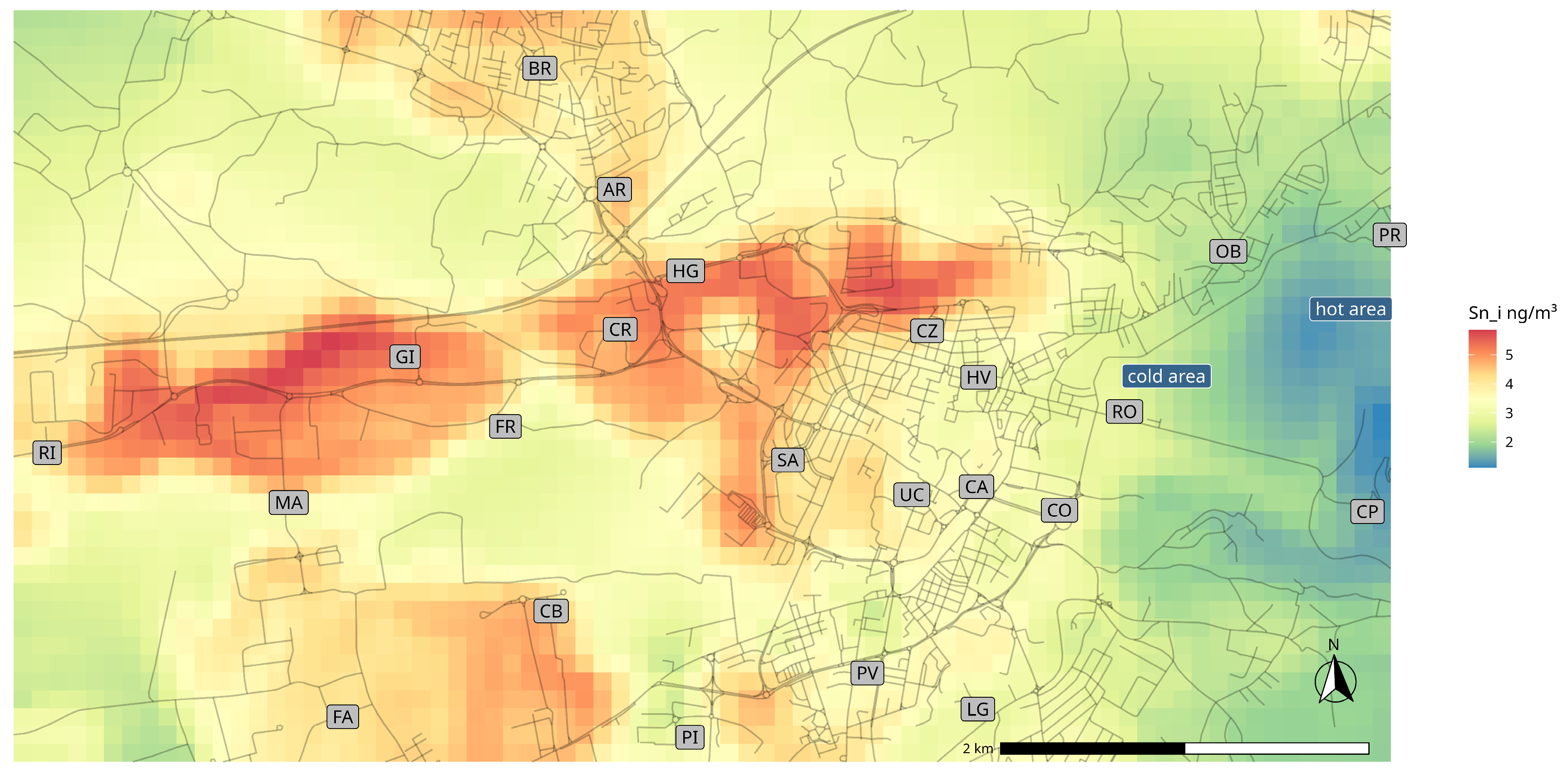
3.1.4. Road Dust
3.1.5. Brake Dust
4. Conclusions
Supplementary Materials
Author Contributions
Funding
Institutional Review Board Statement
Informed Consent Statement
Data Availability Statement
Acknowledgments
Conflicts of Interest
References
- Dockery, D.W.; Pope, C.A., 3rd; Xu, X.; Spengler, J.D.; Ware, J.H.; Fay, M.E.; Ferris, B.G., Jr.; Speizer, F.E. An association between air pollution and mortality in six U.S. cities. N. Engl. J. Med. 1993, 329, 1753–1759. [Google Scholar] [CrossRef] [PubMed]
- Pope, C.A.; Dockery, D.W. Health effects of fine particulate air pollution: Lines that connect. J. Air Waste Manag. Assoc. 2006, 56, 709–742. [Google Scholar] [CrossRef] [PubMed]
- Chen, H.; Goldberg, M.S.; Villeneuve, P.J. A systematic review of the relation between long-term exposure to ambient air pollution and chronic diseases. Rev. Environ. Health 2008, 23, 243–297. [Google Scholar] [CrossRef] [PubMed]
- Hoek, G.; Krishnan, R.M.; Beelen, R.; Peters, A.; Ostro, B.; Brunekreef, B.; Kaufman, J.D. Long-term air pollution exposure and cardio- respiratory mortality: A review. Environ. Health 2013, 12, 43. [Google Scholar] [CrossRef]
- Cesaroni, G.; Badaloni, C.; Gariazzo, C.; Stafoggia, M.; Sozzi, R.; Davoli, M.; Forastiere, F. Long-term exposure to urban air pollution and mortality in a cohort of more than a million adults in Rome. Environ. Health Perspect. 2013, 121, 324–331. [Google Scholar] [CrossRef]
- WHO. WHO Global Air Quality Guidelines: Particulate Matter (PM2.5 and PM10), Ozone, Nitrogen Dioxide, Sulfur Dioxide and Carbon Monoxide; World Health Organization: Geneva, Switzerland, 2021; ISBN 9789240034228/9789240034211 . [Google Scholar]
- European Environment Agency, Harm to Human Health from Air Pollution in Europe—Burden of Disease Status, 2024; Publications Office of the European Union: Luxemburg, 2024; ISBN 978-92-9480-695-6. [CrossRef]
- Beckerman, B.S.; Jerrett, M.; Serre, M.; Martin, R.V.; Lee, S.J.; van Donkelaar, A.; Ross, Z.; Su, J.; Burnett, R.T. A hybrid approach to estimating national scale spatiotemporal variability of PM2.5 in the contiguous United States. Environ. Sci. Technol. 2013, 47, 7233–7241. [Google Scholar] [CrossRef]
- Tsai, M.-Y.; Hoek, G.; Eeftens, M.; de Hoogh, K.; Beelen, R.; Beregszászi, T.; Cesaroni, G.; Cirach, M.; Cyrys, J.; De Nazelle, A.; et al. Spatial variation of PM elemental composition between and within 20 European study areas—Results of the ESCAPE project. Environ. Int. 2015, 84, 181–192. [Google Scholar] [CrossRef]
- Zhang, J.J.Y.; Sun, L.; Barrett, O.; Bertazzon, S.; Underwood, F.E.; Johnson, M. Development of land-use regression models for metals associated with airborne particulate matter in a North American city. Atmos. Environ. 2015, 106, 165–177. [Google Scholar] [CrossRef]
- Lee, M.; Kloog, I.; Chudnovsky, A.; Lyapustin, A.; Wang, Y.; Melly, S.; Coull, B.; Koutrakis, P.; Schwartz, J. Spatiotemporal prediction of fine particulate matter using high-resolution satellite images in the Southeastern US 2003–2011. J. Expo. Sci. Environ. Epidemiol. 2015, 26, 377–384. [Google Scholar] [CrossRef]
- Di, Q.; Kloog, I.; Koutrakis, P.; Lyapustin, A.; Wang, Y.; Schwartz, J. Assessing PM2.5 exposures with high spatiotemporal resolution across the continental United States. Environ. Sci. Technol. 2016, 50, 4712–4721. [Google Scholar] [CrossRef]
- Stafoggia, M.; Schwartz, J.; Badaloni, C.; Bellander, T.; Alessandrini, E.; Cattani, G.; Donato, F.D.; Gaeta, A.; Leone, G.; Lyapustin, A.; et al. Estimation of daily PM10 concentrations in Italy (2006–2012) using finely resolved satellite data, land use variables and meteorology. Environ. Int. 2016, 99, 234–244. [Google Scholar] [CrossRef] [PubMed]
- Gariazzo, C.; Carlino, G.; Silibello, C.; Renzi, M.; Finardi, S.; Pepe, N.; Radice, P.; Forastiere, F.; Michelozzi, P.; Viegi, G.; et al. A multi-city air pollution population exposure study: Combined use of chemical-transport and random-Forest models with dynamic population data. Sci. Total Environ. 2020, 724, 138102. [Google Scholar] [CrossRef] [PubMed]
- Massimi, L.; Ristorini, M.; Simonetti, G.; Frezzini, M.A.; Astolfi, M.L.; Canepari, S. Spatial mapping and size distribution of oxidative potential of particulate matter released by spatially disaggregated sources. Environ. Pollut. 2020, 266, 115271. [Google Scholar] [CrossRef] [PubMed]
- Massimi, L.; Pietrantonio, E.; Astolfi, M.L.; Canepari, S. Innovative experimental approach for spatial mapping of source-specific risk contributions of potentially toxic trace elements in PM10. Chemosphere 2022, 307, 135871. [Google Scholar] [CrossRef]
- EC. Ambient Air Pollution by As, Cd and Ni Compounds; Position Paper; Office for Official Publications of the European Communities: Luxembourg, 2001. [Google Scholar]
- WHO. Air Quality Guidelines for Europe, 2nd ed.; Regional Office for Europe Regional Publications, European Series, n. 91; World Health Organization: Copenhagen, Denmark, 2000. [Google Scholar]
- Potter, N.A.; Meltzer, G.Y.; Avenbuan, O.N.; Raja, A.; Zelikoff, J.T. Particulate Matter and Associated Metals: A Link with Neurotoxicity and Mental Health. Atmosphere 2021, 12, 425. [Google Scholar] [CrossRef]
- IARC. A review of human carcinogens: Part F: Chemical agents and related occupations. In IARC Mono-Graphs on the Evaluation of Carcinogenic Risks to Humans; IARC Working Group on the Evaluation of Carcinogenic Risks to Humans: Lyon, France, 2012; Volume 100F. [Google Scholar]
- Yuan, L.; Zhang, Y.; Gao, Y.; Tian, Y. Maternal fine particulate matter (PM2.5) exposure and adverse birth outcomes: An updated systematic review based on cohort studies. Environ. Sci. Pollut. Res. Int. 2019, 26, 13963–13983. [Google Scholar] [CrossRef]
- Montagne, D.; Hoek, G.; Nieuwenhuijsen, M.; Lanki, T.; Pennanen, A.; Portella, M.; Meliefste, K.; Wang, M.; Eeftens, M.; Yli-Tuomi, T.; et al. The association of LUR modeled PM2.5 elemental composition with personal exposure. Sci. Total Environ. 2014, 493, 298–306. [Google Scholar] [CrossRef]
- Ho, C.-C.; Chan, C.-C.; Cho, C.-W.; Lin, H.-I.; Lee, J.-H.; Wu, C.-F. Land use regression modeling with vertical distribution measurements for fine particulate matter and elements in an urban area. Atmos. Environ. 2015, 104, 256–263. [Google Scholar] [CrossRef]
- Li, H.Z.; Dallmann, T.R.; Gu, P.; Presto, A.A. Application of mobile sampling to investigate spatial variation in fine particle composition. Atmos. Environ. 2016, 142, 71–82. [Google Scholar] [CrossRef]
- Tripathy, S.; Tunno, B.J.; Michanowicz, D.R.; Kinnee, E.; Shmool, J.L.; Gillooly, S.; Clougherty, J.E. Hybrid land use regression modeling for estimating spatio-temporal exposures to PM2.5, BC, and metal components across a metropolitan area of complex terrain and industrial sources. Sci. Total Environ. 2019, 673, 54–63. [Google Scholar] [CrossRef]
- Brokamp, C.; Jandarov, R.; Rao, M.B.; LeMasters, G.; Ryan, P. Exposure assessment models for elemental components of particulate matter in an urban environment: A comparison of regression and random forest approaches. Atmos. Environ. 2017, 151, 1–11. [Google Scholar] [CrossRef] [PubMed]
- Yin, X.; Franklin, M.; Fallah-Shorshani, M.; Shafer, M.; McConnell, R.; Fruin, S. Exposure models for particulate matter elemental concentrations in Southern California. Environ. Int. 2022, 165, 107247. [Google Scholar] [CrossRef] [PubMed]
- Hastie, T.; Tibshirani, R. Generalized Additive Models. Stat. Sci. 1986, 1, 297–310. [Google Scholar] [CrossRef]
- Hastie, T.; Tibshirani, R. Generalized Additive Models; Monographs on Statistics and Applied Probability; Chapman and Hall: London, UK, 1990. [Google Scholar]
- Wood, S.N. Generalized Additive Models: An Introduction with R, 2nd ed.; Chapman & Hall/CRC: New York, NY, USA, 2017. [Google Scholar]
- Carslaw, D.C.; Beevers, S.D.; Tate, J.E. Modelling and assessing trends in traffic-related emissions using a generalised additive modelling approach. Atmos. Environ. 2007, 41, 5289–5299. [Google Scholar] [CrossRef]
- Carslaw, D.C.; Carslaw, N. Detecting and characterising small changes in urban nitrogen dioxide concentrations. Atmos. Environ. 2007, 41, 4723–4733. [Google Scholar] [CrossRef]
- Barmpadimos, I.; Hueglin, C.; Keller, J.; Henne, S.; Prévôt, A.S.H. Influence of meteorology on PM10 trends and variability in Switzerland from 1991 to 2008. Atmos. Chem. Phys. 2011, 11, 1813–1835. [Google Scholar] [CrossRef]
- Ordóñez, C.; Garrido-Perez, J.M.; García-Herrera, R. Early spring near-surface ozone in Europe during the COVID-19 shutdown: Meteorological effects outweigh emission changes. Sci. Total Environ. 2020, 747, 141322. [Google Scholar] [CrossRef]
- Gerling, L.; Wiedensohler, A.; Weber, S. Statistical modelling of spatial and temporal variation in urban particle number size distribution at traffic and background sites. Atmos. Environ. 2021, 244, 117925. [Google Scholar] [CrossRef]
- Hua, J.; Zhang, Y.; de Foy, B.; Shang, J.; Schauer, J.J.; Mei, X.; Sulaymon, I.D.; Han, T. Quantitative estimation of meteorological impacts and the COVID-19 lockdown reductions on NO2 and PM2.5 over the Beijing area using Generalized Additive Models (GAM). J. Environ. Manag. 2021, 291, 112676. [Google Scholar] [CrossRef]
- Gaeta, A.; Leone, G.; Di Menno di Bucchianico, A.; Cusano, M.; Gaddi, R.; Pelliccioni, A.; Reatini, M.A.; Di Bernardino, A.; Cattani, G. Spatio-Temporal Modeling of Small-Scale Ultrafine Particle Variability Using Generalized Additive Models. Sustainability 2022, 14, 313. [Google Scholar] [CrossRef]
- Leone, G.; Cattani, G.; Cusano, M.; Gaeta, A.; Pellis, G.; Vitullo, M.; Morelli, R. Wildfires Impact Assessment on PM Levels Using Generalized Additive Mixed Models. Atmosphere 2023, 14, 231. [Google Scholar] [CrossRef]
- Guan, L.; Liang, Y.; Tian, Y.; Yang, Z.; Sun, Y.; Feng, Y. Quantitatively analyzing effects of meteorology and PM2.5 sources on low visual distance. Sci. Total Environ. 2019, 659, 764–772. [Google Scholar] [CrossRef] [PubMed]
- de Foy, B.; Heo, J.; Kang, J.-Y.; Kim, H.; Schauer, J.J. Source attribution of air pollution using a generalized additive model and particle trajectory clusters. Sci. Total Environ. 2021, 780, 146458. [Google Scholar] [CrossRef] [PubMed]
- Sofowote, U.M.; Healy, R.M.; Su, Y.; Debosz, J.; Noble, M.; Munoz, A.; Jeong, C.-H.; Wang, J.M.; Hilker, N.; Evans, G.J.; et al. Sources, variability and parameterizations of intra-city factors obtained from dispersion-normalized multi-time resolution factor analyses of PM2.5 in an urban environment. Sci. Total Environ. 2021, 761, 143225. [Google Scholar] [CrossRef]
- Matthaios, V.N.; Lawrence, J.; Martins, M.A.G.; Ferguson, S.T.; Wolfson, J.M.; Harrison, R.M.; Koutrakis, P. Quantifying factors affecting contributions of roadway exhaust and non-exhaust emissions to ambient PM10–2.5 and PM2.5–0.2 particles. Sci. Total Environ. 2022, 835, 155368. [Google Scholar] [CrossRef]
- Ferrero, L.; Cappelletti, D.; Moroni, B.; Sangiorgi, G.; Perrone, M.G.; Crocchianti, S.; Bolzacchini, E. Wintertime aerosol dynamics and chemical composition across the mixing layer over basin valleys. Atmos. Environ. 2012, 56, 143–153. [Google Scholar] [CrossRef]
- Peel, M.C.; Finlayson, B.L.; McMahon, T.A. Updated world map of the Köppen-Geiger climate classification. Hydrol. Earth Syst. Sci. Discuss. 2007, 4, 439–473. [Google Scholar] [CrossRef]
- Morini, E.; Touchaei, A.; Castellani, B.; Rossi, F.; Cotana, F. The impact of albedo increase to mitigate the urban heat island in Terni (Italy) using the WRF model. Sustainability 2016, 8, 999. [Google Scholar] [CrossRef]
- Massimi, L.; Ristorini, M.; Eusebio, M.; Florendo, D.; Adeyemo, A.; Brugnoli, D.; Canepari, S. Monitoring and evaluation of Terni (Central Italy) air quality through spatially resolved analyses. Atmosphere 2017, 8, 200. [Google Scholar] [CrossRef]
- Massimi, L.; Ristorini, M.; Astolfi, M.L.; Perrino, C.; Canepari, S. High resolution spatial mapping of element concentrations in PM10: A powerful tool for localization of emission sources. Atmos. Res. 2020, 244, 105060. [Google Scholar] [CrossRef]
- Capelli, L.; Sironi, S.; Del Rosso, R.; Céntola, P.; Rossi, A.; Austeri, C. Olfactometric approach for the evaluation of citizens’ exposure to industrial emissions in the city of Terni, Italy. Sci. Total Environ. 2011, 409, 595–603. [Google Scholar] [CrossRef] [PubMed]
- Guerrini, R. Qualità Dell’aria Nella Provincia di Terni Tra il 2002 e il 2011; Quad ARPA Umbria: Terni, Italy, 2012; pp. 81–87. [Google Scholar]
- Canepari, S.; Astolfi, M.L.; Farao, C.; Maretto, M.; Frasca, D.; Marcoccia, M.; Perrino, C. Seasonal variations in the chemical composition of particulate matter: A case study in the Po Valley. Part II: Concentration and solubility of micro- and trace-elements. Environ. Sci. Pollut. Res. 2014, 21, 4010–4022. [Google Scholar] [CrossRef] [PubMed]
- Canepari, S.; Astolfi, M.L.; Catrambone, M.; Frasca, D.; Marcoccia, M.; Marcovecchio, F.; Massimi, L.; Rantica, E.; Perrino, C. A combined chemical/size fractionation approach to study winter/summer variations, ageing and source strength of atmospheric particles. Environ. Pollut. 2019, 253, 19–28. [Google Scholar] [CrossRef]
- Massimi, L.; Pietrodangelo, A.; Frezzini, M.A.; Ristorini, M.; De Francesco, N.; Sargolini, T.; Perrino, C. Effects of COVID-19 lockdown on PM10 composition and sources in the Rome Area (Italy) by elements’ chemical fractionation-based source apportionment. Atmos. Res. 2022, 266, 105970. [Google Scholar] [CrossRef]
- R Core Team. R: A Language and Environment for Statistical Computing; R Foundation for Statistical Computing: Vienna, Austria, 2024; Available online: https://www.R-project.org/ (accessed on 31 December 2024).
- Zuur, A.F. Beginner’s Guide to Generalized Additive Models with R; Highland Statistics Ltd.: Newburgh, UK, 2012; ISBN 978-0-957-17412-2. Available online: https://www.highstat.com/index.php?view=article&id=20&catid=18 (accessed on 4 April 2025).
- Clifford, S.; Choy, S.L.; Hussein, T.; Mengersen, K.; Morawska, L. Using the Generalised Additive Model to model the particle number count of ultrafine particles. Atmos. Environ. 2011, 45, 5934–5945. [Google Scholar] [CrossRef]
- Wood, S. Package ‘Mgcv’. 2023. Available online: https://cran.r-project.org/web/packages/mgcv/mgcv.pdf (accessed on 21 December 2023).
- Kumar, A.; Luo, J.; Bennett, G. Statistical Evaluation of Lower Flammability Distance (LFD) using Four Hazardous Release. Models. Process Saf. Prog. 1993, 12, 1–11. [Google Scholar] [CrossRef]
- Hanna, S.; Chang, J. Acceptance criteria for urban dispersion model evaluation. Meteorol. Atmos. Phys. 2012, 116, 133–146. [Google Scholar] [CrossRef]
- Querol, X.; Viana, M.; Alastuey, A.; Amato, F.; Moreno, T.; Castillo, S.; Pey, J.; de la Rosa, J.; Sánchez de la Campa, A.; Artíñano, B.; et al. Source origin of trace elements in PM from regional background, urban and industrial sites of Spain. Atmos. Environ. 2007, 41, 7219–7231. [Google Scholar] [CrossRef]
- Owoade, K.O.; Hopke, P.K.; Olise, F.S.; Ogundele, L.T.; Fawole, O.G.; Olaniyi, B.H.; Jegede, O.O.; Ayoola, M.A.; Bashiru, M.I. Chemical compositions and source identification of particulate matter (PM2.5 and PM2.5–10) from a scrap iron and steel smelting industry along the Ife–Ibadan highway, Nigeria. Atmos. Pollut. Res. 2015, 6, 107–119. [Google Scholar] [CrossRef]
- Duan, F.; Liu, X.; Yu, T.; Cachier, H. Identification and estimate of biomass burning contribution to the urban aerosol organic carbon concentrations in Beijing. Atmos. Environ. 2004, 38, 1275–1282. [Google Scholar] [CrossRef]
- Zhang, Z.; Gao, J.; Engling, G.; Tao, J.; Chai, F.; Zhang, L.; Zhang, R.; Sang, X.; Chan, C.; Lin, Z.; et al. Characteristics and applications of size-segregated biomass burning tracers in China’s Pearl River Delta region. Atmos. Environ. 2015, 102, 290–301. [Google Scholar] [CrossRef]
- Frasca, D.; Marcoccia, M.; Tofful, L.; Simonetti, G.; Perrino, C.; Canepari, S. Influence of advanced wood-fired appliances for residential heating on indoor air quality. Chemosphere 2018, 211, 62–71. [Google Scholar] [CrossRef] [PubMed]
- Simonetti, G.; Frasca, D.; Marcoccia, M.; Farao, C.; Canepari, S. Multi-elemental analysis of particulate matter samples collected by a particle-into-liquid sampler. Atmos. Pollut. Res. 2018, 9, 747–754. [Google Scholar] [CrossRef]
- Massimi, L.; Simonetti, G.; Buiarelli, F.; Di Filippo, P.; Pomata, D.; Riccardi, C.; Canepari, S. Spatial distribution of levoglucosan and alternative biomass burning tracers in atmospheric aerosols, in an urban and industrial hot-spot of Central Italy. Atmos. Res. 2020, 239, 104904. [Google Scholar] [CrossRef]
- Samara, C.; Kouimtzis, T.; Tsitouridou, R.; Kanias, G.; Simeonov, V. Chemical mass balance source apportionment of PM10 in an industrialized urban area of Northern Greece. Atmos. Environ. 2003, 37, 41–54. [Google Scholar] [CrossRef]
- Amato, F.; Pandolfi, M.; Viana, M.; Querol, X.; Alastuey, A.; Moreno, T. Spatial and chemical patterns of PM10 in road dust deposited in urban environment. Atmos. Environ. 2009, 43, 1650–1659. [Google Scholar] [CrossRef]
- Pant, P.; Harrison, R.M. Estimation of the contribution of road traffic emissions to particulate matter concentrations from field measurements: A review. Atmos. Environ. 2013, 77, 78–97. [Google Scholar] [CrossRef]
- Bencharif-Madani, F.; Ali-Khodja, H.; Kemmouche, A.; Terrouche, A.; Lokorai, K.; Naidja, L.; Bouziane, M. Mass concentrations, seasonal variations, chemical compositions and element sources of PM10 at an urban site in Constantine, Northeast Algeria. J. Geochem. Explor. 2019, 206, 106356. [Google Scholar] [CrossRef]
- Soleimanian, E.; Taghvaee, S.; Mousavi, A.; Sowlat, M.H.; Hassanvand, M.S.; Yunesian, M.; Naddafi, K.; Sioutas, C. Sources and temporal variations of coarse particulate matter (PM) in central Tehran, Iran. Atmosphere 2019, 10, 291. [Google Scholar] [CrossRef]
- Perrino, C.; Catrambone, M.; Canepari, S. Chemical composition of PM10 in 16 urban, industrial and background sites in Italy. Atmosphere 2020, 11, 479. [Google Scholar] [CrossRef]
- Weckwerth, G. Verification of traffic emitted aerosol components in the ambient air of Cologne (Germany). Atmos. Environ. 2001, 35, 5525–5536. [Google Scholar] [CrossRef]
- Abbasi, S.; Olander, L.; Larsson, C.; Olofsson, U.; Jansson, A.; Sellgren, U. A field test study of airborne wear particles from a running regional train. Proc. IMechE Part F J. Rail Rapid Transit. 2012, 226, 95–109. [Google Scholar] [CrossRef]
- Querol, X.; Moreno, T.; Karanasiou, A.; Reche, C.; Alastuey, A.; Viana, M.; Font, O.; Gil, J.; de Miguel, E.; Capdevila, M. Variability of levels and composition of PM10 and PM2.5 in the Barcelona metro system. Atmos. Chem. Phys. 2012, 12, 5055–5076. [Google Scholar] [CrossRef]
- Kam, W.; Delfino, R.J.; Schauer, J.J.; Sioutas, C. A comparative assessment of PM2.5 exposures in light-rail, subway, freeway, and surface street environments in Los Angeles and estimated lung cancer risk. Environ. Sci. Process. Impacts 2013, 15, 234–243. [Google Scholar] [CrossRef]
- Namgung, H.G.; Kim, J.B.; Woo, S.H.; Park, S.; Kim, M.; Kim, M.S.; Bae, G.N.; Park, D.; Kwon, S.B. Generation of nanoparticles from friction between railway brake disks and pads. Environ. Sci. Technol. 2016, 50, 3453–3461. [Google Scholar] [CrossRef]
- Ma, X.; Zou, B.; Deng, J.; Gao, J.; Longley, I.; Xiao, S.; Guo, B.; Wu, Y.; Xu, T.; Xu, X.; et al. A comprehensive review of the development of land use regression approaches for modeling spatiotemporal variations of ambient air pollution: A perspective from 2011 to 2023. Environ. Int. 2024, 183, 108430. [Google Scholar] [CrossRef]


| FAC2 | |FB| | NMSE |
|---|---|---|
| ≥0.50 | ≤0.30 | ≤3 |
| Variable 1 | Description | Unit of Measure |
|---|---|---|
| code_12100 | Industrial, commercial, and public areas | m2 |
| code_12220 | Local street area | m2 |
| bh_index | Height of the buildings weighted on the related area of the urban fabric | m/m2 |
| dist_ferr | Distance from railway | m |
| imp_200 | Impermeable surfaces in a buffer of 200 m | % |
| pop_200 | Number of inhabitants in a buffer of 200 m | n. |
| dist_strade | Distance of the nearest road | m |
| ml_200 | Lengths of road in a buffer of 200 m | m |
| cold_area | Distance from cold area of the steel plant | m |
| hot_area | Distance from the hot area of the steel plant | m |
| Variable 1 | Description | Unit of Measure |
|---|---|---|
| t2m_mean | Mean, over the air quality sampling periods, of the air temperature at 2 m from ground level | °C |
| tmin2m_mean | Mean of the daily minimum air temperature at 2 m from ground level | °C |
| tmax2m_mean | Mean of the daily maximum air temperature at 2 m from ground level | °C |
| tp_mean | Mean of the daily accumulated precipitation at 2 m from ground level | mm |
| rh_mean | Mean of the relative humidity of the air at 2 m from ground | % |
| u10m_mean | Mean of the eastward horizontal wind component at 10 m height | m/s |
| v10m_mean | Mean of the northward vertical wind component at 10 m height | m/s |
| wspeed_mean | Mean of the wind speed intensity at 10 m height | m/s |
| wspeed_max_mean | Mean of the daily maximum wind speed intensity at 10 m height | m/s |
| sp_mean | Mean ground level pressure | hPa |
| nirradiance_mean | Mean solar radiation intensity | W/mq |
| pbl00_mean | Mean of the planetary boundary layer height at 00:00 | km |
| pbl12_mean | Mean of the planetary boundary layer height at 12:00 | km |
| pblmin_mean | Mean of the minimum planetary boundary layer height | km |
| pblmax_mean | Mean of the maximum planetary boundary layer height | km |
| Pollutant | Model Formula * |
|---|---|
| PM10 | value ~ s(pbl00) + s(wspeed_max) + s(pop, k = 1) + s(code_12100, k = 1) + s(sp) + s(rh) + s(hot_area, k = 6) |
| Bi_i | value ~ s(rh) + s(hot_area, k = 6) + s(code_12100, k = 1) + s(v10m) + s(wspeed) + s(imp, k = 1) |
| Cr_i | value ~ s(cold_area, k = 6) + s(u10m) |
| Cr_s | value ~ s(hot_area, k = 6) + s(rh) + s(dist_ferr, k = 1) + s(code_12100, k = 1) + s(dist_strade, k = 1, bs = “gp”) + s(imp, k = 1) |
| Cs_s | value ~ season + s(u10m) + s(cold_area, k = 6) + s(dist_ferr, k = 1) + s(ml, k = 1) + s(sp) + s(code_12100, k = 1) |
| Cu_i | value ~ s(u10m) + s(code_12100, k = 1) + s(code_12220, k = 1) + s(v10m) + s(pblmin) |
| Fe_i | value ~ s(cold_area, k = 6) + s(u10m) + s(code_12100, k = 1) + s(dist_ferr, k = 1) + s(v10m) |
| K_s | value ~ season + s(pblmax) + s(hot_area, k = 6) + s(dist_ferr, k = 1) + s(bh_index, k = 1) |
| Li_i | value ~ s(pbl12) + s(imp, k = 1) + s(wspeed_max) + s(bh_index, k = 1) |
| Li_s | value ~ s(hot_area, k = 6) + s(rh) + s(dist_ferr, k = 1) + s(pop, k = 1) + s(code_12220, k = 1) |
| Mn_i | value ~ s(cold_area, k = 6) + s(dist_ferr, k = 1) + s(wspeed_max) + s(imp, k = 1) + s(pop, k = 1) + s(pblmin) + s(dist_strade, k = 1, bs = “gp”) |
| Mn_s | value ~ s(nirradiance) + s(hot_area, k = 6) + s(dist_ferr, k = 1) + s(code_12220, k = 1) + s(pop, k = 1) + s(pbl00) |
| Mo_s | value ~ s(cold_area, k = 6) + s(wspeed_max) + s(pbl00) |
| Ni_i | value ~ s(cold_area, k = 6) + s(tmin2m) + s(wspeed_max) + s(tp) |
| Pb_i | value ~ season + s(hot_area, k = 6) + s(dist_ferr, k = 1) + s(t2m) + s(code_12220, k = 1) + s(pop, k = 1) |
| Sn_i | value ~ s(pbl12) + s(hot_area, k = 6) + s(dist_ferr, k = 1) + s(bh_index, k = 1) + s(imp, k = 1) |
| Tl_s | value ~ season + s(hot_area, k = 6) + s(sp) + s(bh_index, k = 1) + s(dist_ferr, k = 1) + s(imp, k = 1) |
| W_s | value ~ s(cold_area, k = 6) + s(v10m) |
| Zn_s | value ~ s(pblmax) + s(hot_area, k = 6) + s(dist_ferr, k = 1) + s(code_12220, k = 1) + s(pop, k = 1) |
| Zr_i | value ~ s(code_12220, k = 1) + s(pblmax) + s(bh_index, k = 1) + s(cold_area, k = 6) + s(imp, k = 1) + s(dist_ferr, k = 1) + s(wspeed_max) |
| Pollutant | Adj R2 | CV-R2 | RMSE | FAC2 | FB | NMSE |
|---|---|---|---|---|---|---|
| PM10 | 0.80 | 0.81 | 6.59 | 1.00 | 0.09 | 0.05 |
| Bi_i | 0.79 | 0.80 | 0.08 | 0.84 | 0.20 | 0.14 |
| Cd_s | 0.74 | 0.75 | 0.06 | 0.87 | 0.16 | 0.13 |
| Cr_i | 0.68 | 0.69 | 19.32 | 0.78 | 0.23 | 0.43 |
| Cr_s | 0.70 | 0.72 | 0.76 | 0.89 | 0.16 | 0.18 |
| Cs_s | 0.86 | 0.87 | 0.01 | 0.91 | 0.16 | 0.08 |
| Cu_i | 0.63 | 0.65 | 3.29 | 0.94 | 0.21 | 0.13 |
| Fe_i | 0.56 | 0.59 | 223.08 | 0.90 | 0.22 | 0.20 |
| K_s | 0.84 | 0.84 | 124.49 | 0.93 | 0.13 | 0.09 |
| Li_i | 0.56 | 0.58 | 0.04 | 0.92 | 0.12 | 0.12 |
| Li_s | 0.74 | 0.76 | 0.04 | 0.95 | 0.14 | 0.09 |
| Mn_i | 0.69 | 0.71 | 3.36 | 0.97 | 0.12 | 0.09 |
| Mn_s | 0.71 | 0.73 | 2.26 | 0.95 | 0.16 | 0.12 |
| Mo_s | 0.83 | 0.82 | 4.35 | 0.76 | 0.26 | 0.47 |
| Ni_i | 0.81 | 0.81 | 8.54 | 0.74 | 0.27 | 0.57 |
| Pb_i | 0.75 | 0.77 | 1.61 | 0.92 | 0.20 | 0.14 |
| Rb_s | 0.72 | 0.73 | 0.38 | 0.91 | 0.14 | 0.13 |
| Sn_i | 0.88 | 0.89 | 1.01 | 0.91 | 0.23 | 0.10 |
| Tl_s | 0.86 | 0.87 | 0.03 | 0.92 | 0.18 | 0.10 |
| W_s | 0.85 | 0.85 | 0.04 | 0.77 | 0.24 | 0.37 |
| Zn_s | 0.73 | 0.75 | 10.44 | 0.91 | 0.16 | 0.12 |
| Zr_i | 0.56 | 0.59 | 0.59 | 0.21 | 0.87 | 0.19 |
Disclaimer/Publisher’s Note: The statements, opinions and data contained in all publications are solely those of the individual author(s) and contributor(s) and not of MDPI and/or the editor(s). MDPI and/or the editor(s) disclaim responsibility for any injury to people or property resulting from any ideas, methods, instructions or products referred to in the content. |
© 2025 by the authors. Licensee MDPI, Basel, Switzerland. This article is an open access article distributed under the terms and conditions of the Creative Commons Attribution (CC BY) license (https://creativecommons.org/licenses/by/4.0/).
Share and Cite
Cusano, M.; Gaeta, A.; Morelli, R.; Cattani, G.; Canepari, S.; Massimi, L.; Leone, G. Spatial Modeling of Trace Element Concentrations in PM10 Using Generalized Additive Models (GAMs). Atmosphere 2025, 16, 464. https://doi.org/10.3390/atmos16040464
Cusano M, Gaeta A, Morelli R, Cattani G, Canepari S, Massimi L, Leone G. Spatial Modeling of Trace Element Concentrations in PM10 Using Generalized Additive Models (GAMs). Atmosphere. 2025; 16(4):464. https://doi.org/10.3390/atmos16040464
Chicago/Turabian StyleCusano, Mariacarmela, Alessandra Gaeta, Raffaele Morelli, Giorgio Cattani, Silvia Canepari, Lorenzo Massimi, and Gianluca Leone. 2025. "Spatial Modeling of Trace Element Concentrations in PM10 Using Generalized Additive Models (GAMs)" Atmosphere 16, no. 4: 464. https://doi.org/10.3390/atmos16040464
APA StyleCusano, M., Gaeta, A., Morelli, R., Cattani, G., Canepari, S., Massimi, L., & Leone, G. (2025). Spatial Modeling of Trace Element Concentrations in PM10 Using Generalized Additive Models (GAMs). Atmosphere, 16(4), 464. https://doi.org/10.3390/atmos16040464