Abstract
In realistic water resource planning, fuzzy constraints can be violated but still allowed to certain acceptance degrees. To address this issue, in this study, a bi-objective pseudo-interval type 2 (T2) linear programming approach with a ranking order relation between the intervals is proposed for water system allocation. This developed approach can transform normal T2 fuzzy sets, including both trapezoidal and triangular types, into the bi-objective linear programming approach solved with the proposed algorithm with mathematical rigor, which improves the flexibility of the decision supports. The new model is applied in the utilization of regional water resource management in Xiamen city, China. Concurrently, a local water system model is established by considering the aspects of industrial, agricultural, and municipal requirements. Thus, by analysis of the solution algorithm, decision-makers can obtain different optimal results by selecting different acceptance degrees. The results also demonstrate the superiority of the proposed method. Therefore, this approach not only augments the theory of the optimal allocation method in water resource management, but also provides the support for meeting the requirements of the 13th five-year plan for Xiamen ecological planning.
1. Introduction
With the rapid development of the social economy and high growth of the world population, a shortage in water resources is unavoidable. Therefore, it is necessary to rationally allocate water resources and make full use of the limited resources [1,2,3,4]. However, in the process of water resource management, there are numerous environmental, social, and economic factors and other uncertain information parameters, which introduce unpredictable uncertainties in the management of water resources [5,6]. Concurrently, there are mutual constraints between the uncertain social economic and environmental factors in the water resource allocation system. These mutual constraints make the process continuous but variant in the water resource management system [7]. Analyzing the effect of each factor in the water management model on the system and determining its degree of impact can provide a decision-making basis for water resource managers [8]. Therefore, rational optimization of water resource management should consider the uncertainties posed by these other factors.
In this area, numerous optimization research studies have been performed to meet the demands of socio-economic development. In the 1940s, researchers began to use optimization methods to solve the problem of reservoir scheduling. Early studies mainly used system analysis methods for achieving a reasonable allocation of water resources [9]. However, there is uncertainty in the spatial and temporal changes in the water supply and their relationship, so that the required water allocation patterns can change over different periods. In more recent years, many studies on the uncertain algorithms for water resource systems have been proposed to deal with such uncertainties existing in the process of decision-making [10,11,12,13,14,15]. For example, an actual water resource management will include meeting the administrative needs, economic needs, security guarantees, and humanistic needs. These demands are typically subject to various interventions, and thus, there are large fluctuations within a certain range in the usage patterns. These uncertain factors are typically expressed as linguistic factors and dynamic processes. Thus, the coefficients in the water system models are generally shown as fuzzy, interval, and/or stochastic uncertainties [16]. Although conventional optimal methods have seemed to be effective for water planning in the past, they still have some limitations and are unable to satisfy their complex social needs. Concurrently, both the environmental regulations and economic needs for water usage usually require the orientation of each respective need individually. The efforts for the maximization of the economic profit may be at the cost of environmental policies. For example, industries need to consider wastewater treatment requirements when they use a certain amount of water sources. This problem often involves multiple conflicting objectives, for which there exists no feasible solution that simultaneously optimizes all the objectives [17]. Therefore, the decision-makers (DMs) have to completely understand the factors that are traded-off before making the decisions. Thus, with formal optimal methods it is impossible to improve the value of the objective without the dissatisfaction of other constraints [18,19]. Consequently, the bi-objective linear program (BOLP) was developed for satisfying the multiple objective demands in system engineering problems. For example, Naderi and Psihvaee [20] introduced a bi-objective robust optimization approach for adjusting the level of reliability for municipal water supply system redesign and rehabilitation problem. Their solutions indicated that neglecting uncertainty can significantly increase the system cost and lead to unsatisfied demands. Irawan et al. [21] proposed a bi-objective optimization programming approach to deal with the conflicting objectives of installation and scheduling on an offshore wind farm. The proposed model was employed to determine the optimal installation schedule considering several constraints such as weather conditions and availability of vessels. The solutions of the bi-objective programming, involving two objectives—namely, minimization of both the total installation cost and total completion period—yielded good results within a reasonable computing time. Belmonte et al. [22] developed a bi-objective mixed-integer linear programming approach, with profit and carbon sequestration serving as the objective functions. The optimal results of the bi-integer approach in which the system-prescribed limits for the contaminants were calculated and met the requirements.
Although BOLP has a one-sided advantage of solving such problems with conflicting objectives, its single framework cannot entirely handle the uncertain coefficients present in the allocation process [23]. BOLP is incapable of mimicking the distribution of water resources under conditions such as floods, droughts, and other catastrophic situations. It also cannot determine the degree of effect of various uncertain factors on the water resource system. Moreover, water resource management is an uncertain, complex, and dynamic process. The existing BOLP model cannot reflect the degree of satisfaction of an objective function and the feasibility of the constraints. Therefore, comprehensive analysis of the uncertainty impact on the water resource system by mathematical methods, coupling with the development of uncertain coefficients—fuzzy or interval or stochastic—can effectively provide DMs with a reasonable water management schedule for sustainable social development. Even if the most basic water allocation system is employed, the seasonal fluctuations in the water resources will cause the program to utilize the uncertainty algorithms for completing the data processing process. For example, Vahdani [23] developed a bi-objective approach, which the embedded interval fuzzy possibilities chance-constraint method for demonstrating the applicability of BOLP in uncertainty. However, the solutions of the Vahdani method will generate numerous objective functions and constraints in the model, so that it will be very difficult to solve and understand the method.
There are numerous fuzzy linear programming methods for the communication of fuzzy sets (FSs) under uncertainty, e.g., the interval fuzzy linear program [24], fully fuzzy linear program [25], fuzzy bi-level linear program [26], fuzzy multi-level program [27], fuzzy multi-objective linear program [28], and hesitant fuzzy mathematical program [29]. However, these methods either transfer FSs into a crisp linear programming model or set excessive constraints or objective functions. Such changes can easily cause distortion or a loss of generality along with a significant increase in the workforce cost. To better solve these issues present in the uncertain linear program, the motivation of this study is to develop a new algorithm applied with the type-2 (T2) fuzzy linear program. However, in the area of water resource management, as an extension concept of FSs, the bi-objective interval T2 FS method is not reported either in the bi-objective program or fuzzy linear program. More essentially, the new method will deliberate on the acceptance degrees at which the fuzzy constraints may be violated, so that the results are accepted even when the constraints might be not satisfied under realistic conditions.
Therefore, the purpose of this study is to newly attempt to investigate a novel bi-objective interval T2 linear programming approach for a real case of water system allocation in Xiamen city in China under multiple uncertainties. The developed model will integrate the interval T2 FS linear programming and BOLP in an optimal framework. The novel model sufficiently reflects the acceptance degree of the fuzzy constraints even if they are violated. It can enhance the flexibility of the process of water allocation. In addition, the developed model can treat the higher levels of FSs in which the traditional fuzzy linear program can easily cause significant distortion or loss of information during the allocation process. The developed model can offer the DMs solutions when the fuzzy constraints may sometimes not be satisfied in reality. Moreover, this new program combines the advantages of the T2 FSs for making the decision process more accurate and detailed than the previous programs. Overall, the advantages of the proposed model can be summarized as follows: (a) the bi-objective interval T2 method is integrated into a previous fuzzy linear programming framework; (b) the fuzzy ranking order relationship method can improve the process of conventional solution steps; (c) the developed interval bi-objective T2 linear model is applied to Xiamen, where there is a shortage of city water, for municipal water resource management. In this process, the wastewater treatment rates are labeled, which is a concrete manifestation of meeting the requirements of the 13th five-year plan for Xiamen ecological planning.
2. Methodology
In this section, the concepts of the interval fuzzy order relation, BOLP, T2 FS linear program, and bi-objective pseudo-interval T2 linear program will be introduced for further convenience.
2.1. Order Relations for Interval Fuzzy Sets
In the framework of the fuzzy optimal linear model, Zadeh [30] defined a fuzzy relation between coefficients and in the theory of FSs. Similarly, Huang [31] defined intervals and with known upper and lower bounds but unknown distribution information. As in previous years, Hu et al. [32] proved the fuzzy partial-order relation between the intervals. More recently, Dong et al. [33] developed fuzzy linear program re-coupled fuzzy and intervals concepts. According to their theories, the membership degree of the fuzzy relation, , can be re-defined as follows:
Definition 1.
Letdenotinganddenotingbe two intervals. The premise,, is regarded as an FS. Accordingly, the membership degree of the upper boundary of the interval is defined as
where is a fuzzy number less than one, reflecting the reality that interval is slightly smaller than interval .
Similarly, the membership degree of the lower boundary of the interval, , can be defined as
where is a fuzzy number larger than zero, which implies that interval is slightly larger than interval .
Therefore, the above definition sets up the quantitative methods for obtaining a certainty degree of membership for the intervals. Thus, the equivalent forms of the interval inequality relations are introduced by satisfying fuzzy ranking index . Thus, the interval inequality relation can be defined as follows:
Definition 2.
A satisfactory crisp equivalent form of an upper boundary of the interval inequality relationis defined as
where denotes the acceptance degree of the interval inequality constraint. It may have the possibility to violate. Thereby, a satisfactory crisp equivalent form of the lower boundary of the interval inequality relation, , is defined as
Thus, according to the lower and upper membership functions, the interval relation, , has a certain acceptance degree of the violated interval relation, , in Equations (3) and (4). Thus, if acceptance degree , the violated relation absolutely cannot be accepted. Concurrently, if acceptance degree , then it represents that interval relation no longer be established. Accordingly, when degree is larger than 0 but less than 1, the DMs allow the interval relation, , to exist with a certain degree of violation. Similarly, the same explanations can be applied to interval relation .
2.2. Bi-Objective Linear Program
According to the research by Ishibuchi and Tanaka [34], BOLP with interval functions can be introduced as follows:
Definition 3.
Let objective coefficient(i = 1, 2, …, m) be defined in intervals. Thus, linear programming with an interval objective function can be formulated as
subject to
Thus, from previous research, Equation (5) can be rewritten as BOLP as
subject to
where X is a set of constraints, which variable x should satisfy the requirements of actual scenarios.
2.3. T2 Fuzzy Set and Its Order Relations
As an extension concept of FSs, the T2 FSs were introduced by Karnik and Mendel [35]. The membership function of the T2 FSs was embedded with an FS to answer the question of the levels of uncertainty. Thus, T2 FSs for the right-hand coefficients have been defined as
Definition 4.
(Uncertain parameter):Consider technological coefficientof a linear program similar to the interval T2 FS. The membership function, which represents the fuzzy space is:
where denotes an interval in (0, 1) and denotes the union over all admissible x and u.
Definition 5.
(Crisp bounds of an ): Consider left to right interval T2 FSs with certain membership functions for both the upper and lower boundaries. Thus, and can be denoted as the left and right interval-valued bounds of Equation (7), respectively. In addition, let bounds of be defined as the boundaries of the α-cuts of the shapes of each left to right FS as
Thus, Equation (8) can be rewritten
Definition 6.
Let T2 FSequate toandequate to. Both of the coefficients denote the interval T2 FSs. Then, according to the previous equation, the order relations betweenandare stipulated as
where , .
2.4. Pseudo-Interval T2 Fuzzy Sets Linear Program
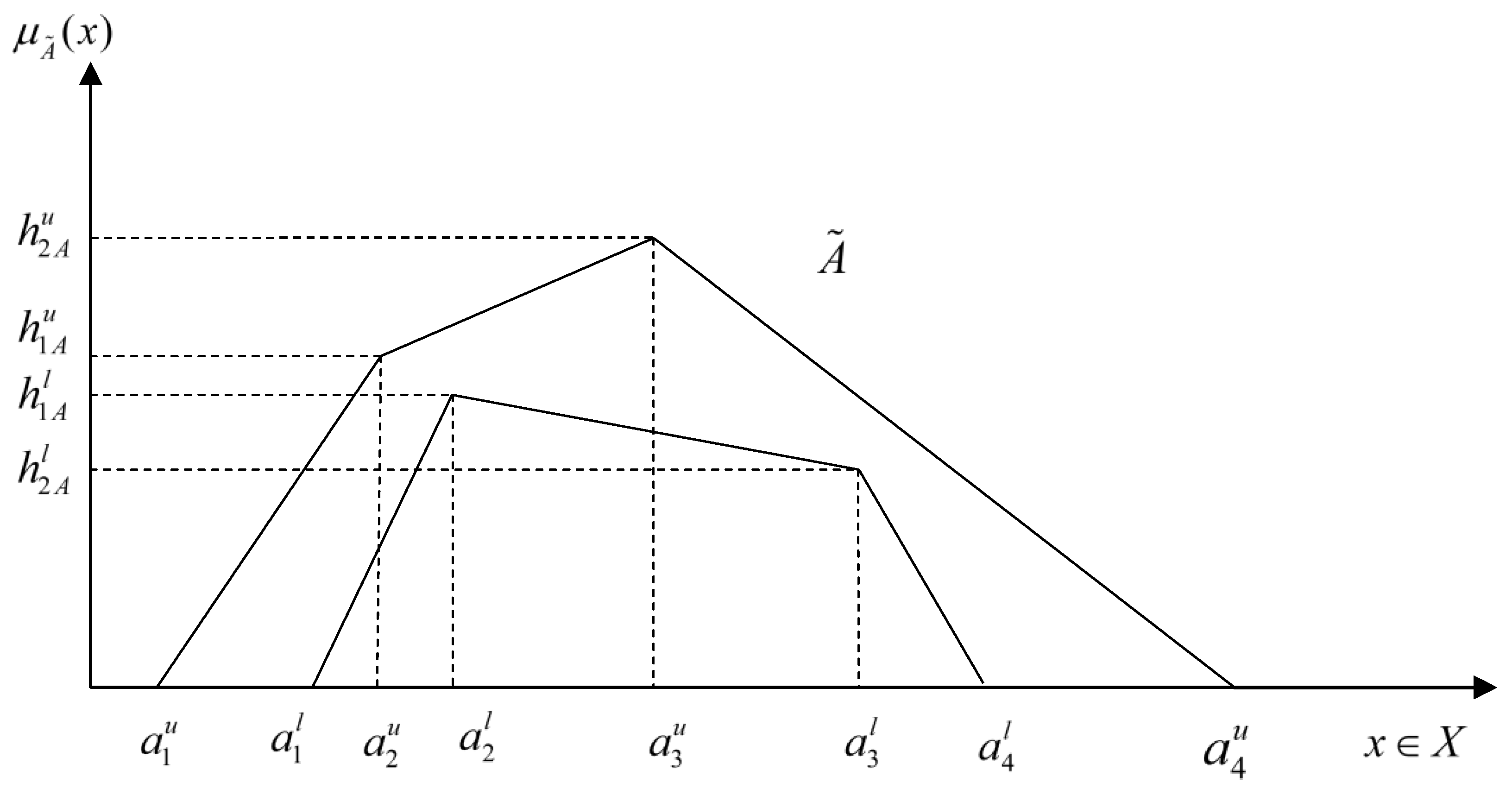
Pseudo-Interval T2 FSs play a central role in the models for their engineering applications [36]. They are a distinct type of FSs that can be described by a trapezoidal shape. Figure 1 shows the general interval T2 trapezoidal FSs. According to [37], the pseudo-interval T2 FS linear program can be described as
subject to
where is the technological coefficient matrix, is the resource coefficient of the right hand side, is the objective coefficient, and is the decision variable coefficient. , , and (i = 1, 2, …, m; j = 1, 2, …, n) denote interval T2 FSs.
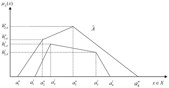
Figure 1.
A general interval type 2 fuzzy set.
Thus, the trapezoidal fuzzy linear program in Equation (11) can be rewritten as
subject to
where , , and denote the interval expectation coefficients as well as the matrix of the corresponding T2 FSs. To solve Equation (11), Definition 2 is employed to deal with the system of interval inequalities, i.e., .
2.5. Bi-Objective Pseudo-Interval T2 Linear Program
According the above statement, thus, the bi-objective pseudo-interval T2 linear programming can be transformed from the Equations (12) to the model as
subject to
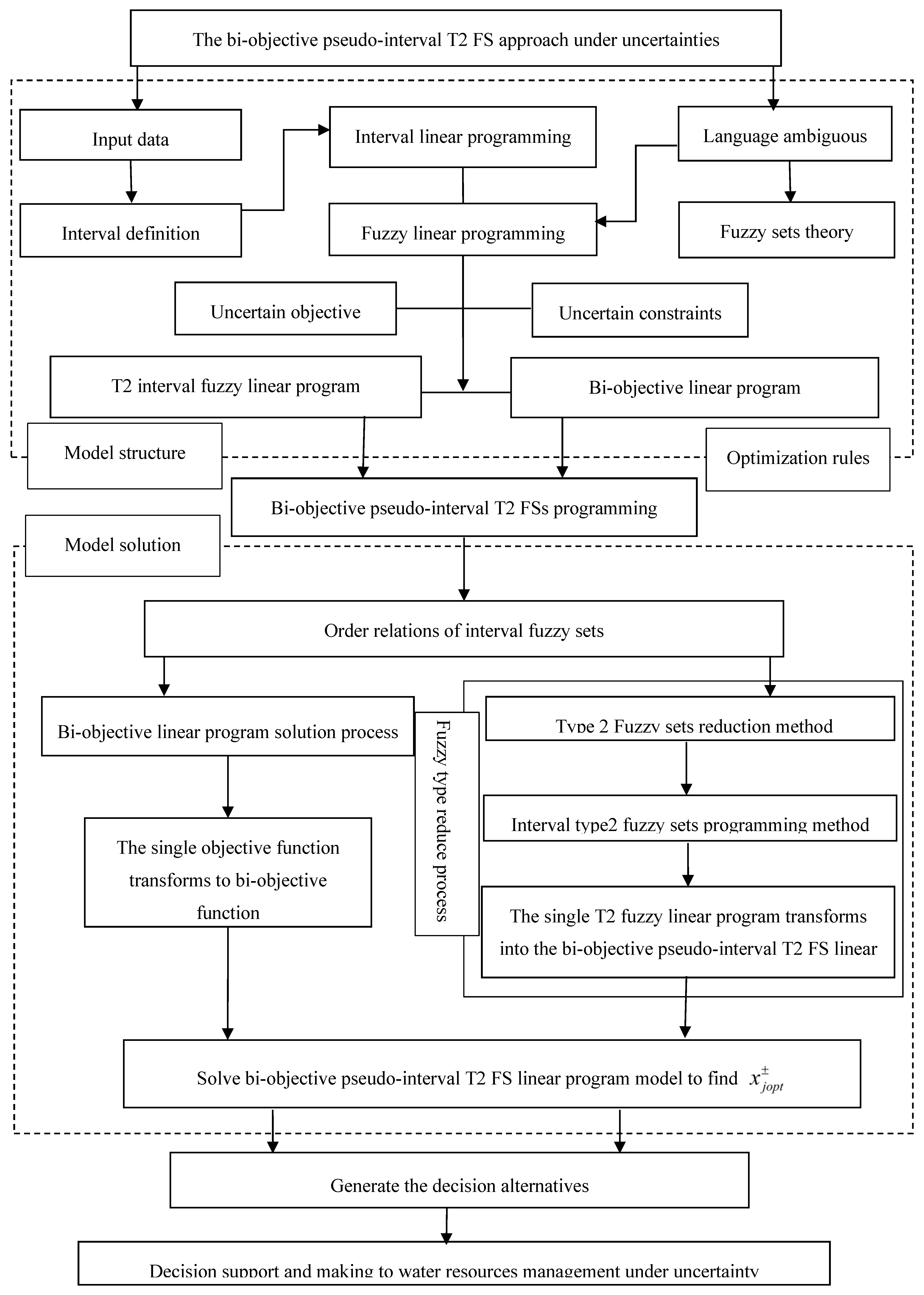
Then the final solution can be obtained as and . The flow diagram, Figure 2, represents the clear details of the methodology. Briefly, the procedure formulation of the bi-objective pseudo-interval T2 FSs linear programming model can be summarized as follows:
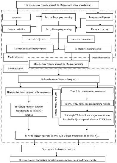
Figure 2.
Flow chart of developed approach model.
Step 1—The interval fuzzy linear program is formulated.
Step 2—The membership function for the interval FSs is defined.
Step 3—The single objective function is transformed into the bi-objective function.
Step 4—Define the order relations for all coefficients of T2 interval fuzzy sets.
Step 5—The single T2 fuzzy linear program is transformed into the bi-objective pseudo-interval T2 FS linear program.
Step 6—The bi-objective pseudo-interval T2 FS is solved by applying the order relations.
3. Case Study
3.1. Overview
Xiamen is affiliated to the Fujian province. It is also known as the “Egret Island”. Xiamen is a sub-provincial city and special economic zone. It is an important central city in the southeast coastal areas of China. It also a port and scenic tourist city. Xiamen is located in the southeastern corner of Fujian province, bordering with Zhangzhou in the west and Nanan and Jinjiang in the north. It faces the Jinmen and Dadan island across the sea in the southeast. It is the main city in the southern Fujian province and also known to form the Golden Triangle Economic Zone with Zhangzhou and Quanzhou.
The total land area of Xiamen is 1699.39 square kilometers. In 2015, the total household population of Xiamen was 2,111,500, of which the urban population was 1,681,800 and rural population was 429,700. The GDP of the entire year was 346.601 billion yuan, of which the added values of the primary and secondary industries were 23.94. 100 million yuan and 150.89 billion yuan (industrial value added was 125.046 billion-yuan, construction industry added value was 23.932 billion yuan), respectively, tertiary industry added value was 193.308 billion yuan, and industrial output value was 503.081 billion yuan (cited).
In this year, the average rainfall in the city was 1622.1 mm, corresponding to an increase of approximately 7.19% on an average over the years. The surface water resources, groundwater resources, and total water resources of Xiamen amounted to 1.374 billion cubic meters, 260.9 million cubic meters, and 1.388 billion cubic meters, respectively. At the end of the year 2015, compared with the end of the previous year, the storage capacity of the medium-sized and major small reservoirs increased by 49.013 million cubic meters. Out of this, the storage capacity increase by 31.956 million cubic meters and 705.7 cubic meters was for medium-sized reservoirs and main small reservoirs, respectively.
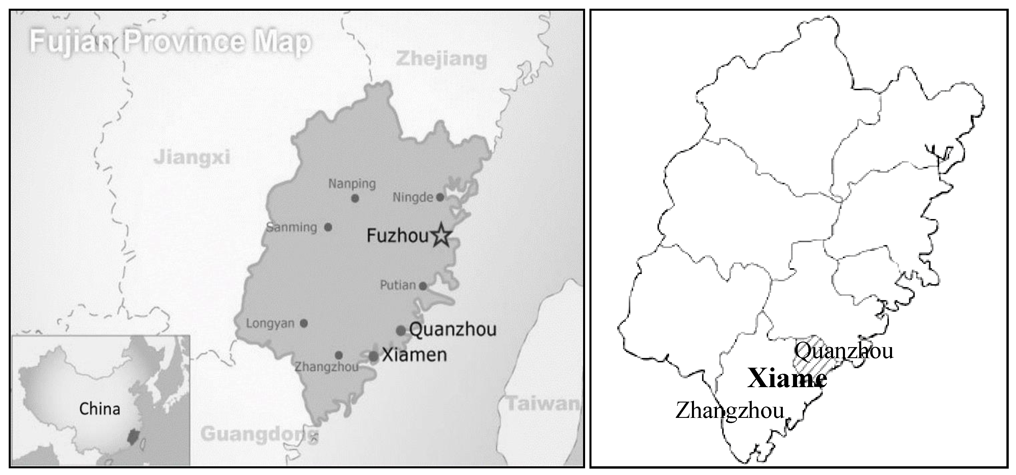
The annual water supply of the city is 63.073 million cubic meters, of which 59.342 million cubic meters comes from the largest surface water supply, accounting for 94.09% of the total water supply. The urban residents have the largest amount of water consumption, which is 181.57 million cubic meters, 28.79% of the total water consumption. The test results from the water quality monitoring site of the city show that the water quality of the drinking water sources and most of the important water bodies in the city is up to the standard. Except for a few, most of the river sections have been polluted to varying degrees. Figure 3 displays the location of Xiamen city in the Fujian province of China.
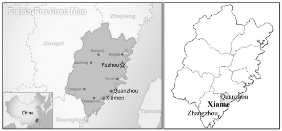
Figure 3.
The location of Xiamen in Fujian province.
3.2. Model Framework
In the model framework described in this section, the assumption was that the historical influence of the local water resources was limited. Although in some cases, the planning model may have been constructed based on nonlinear points, this work uses a linear function and constraints instead of nonlinear functions to avoid the intrinsic nonlinear physical characteristics in the small-scope problems of water allocation. A few model coefficients were given as crisp numbers owing to the data collection process of the Xiamen Statistics Bureau [38]. Table 1, Table 2 and Table 3 present the data collected from a reference book. Based on the analysis of the scale and structure of the industry and characteristics of the water and water sources of Xiamen, a water resource allocation optimization model was constructed as
subject to

Table 1.
Water planning targets for users (106 m3).

Table 2.
Available and demand water with T2 fuzzy features under different inflow levels.

Table 3.
Local economic parameters used in the water system model.
Water quality constraints,
Water consumption constraints,
Reused water capacity,
Sewage treatment constraints,
Non-negative constraints.
In the above-mentioned water planning model, the procedure for converting from the T2 fuzzy linear programming model to the BOLP model can be re-written as Equations (15) to (16), which are mathematically rigorous because they ingeniously combine the fuzzy order relation with the objective program. By this mathematical transformation, this newly developed model can solve both the trapezoidal and triangular fuzzy linear programming models. This implies that the wider application process can increase the diversity and accuracy of the decision supports.
According to the processes in Equation (13) and objective functions in (15), the first objective function can be rewritten as
Thus, the second objective function can be rewritten as
Based on the superiority of the novel methods, the model can be solved by a linear programming software through the following process: (1) the acceptance degree for the DMs is selected; (2) the optimal results of the model are obtained; (3) the optimal values of the objective function as well as the coefficients are captured; (4) the global optimal solution of the water planning for Xiamen city is derived.
4. Results and Discussion
4.1. Bi-Objective Water Model Solutions
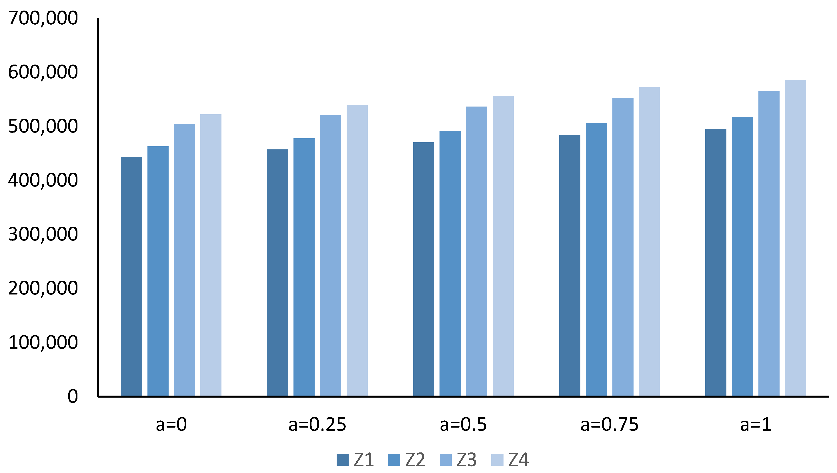
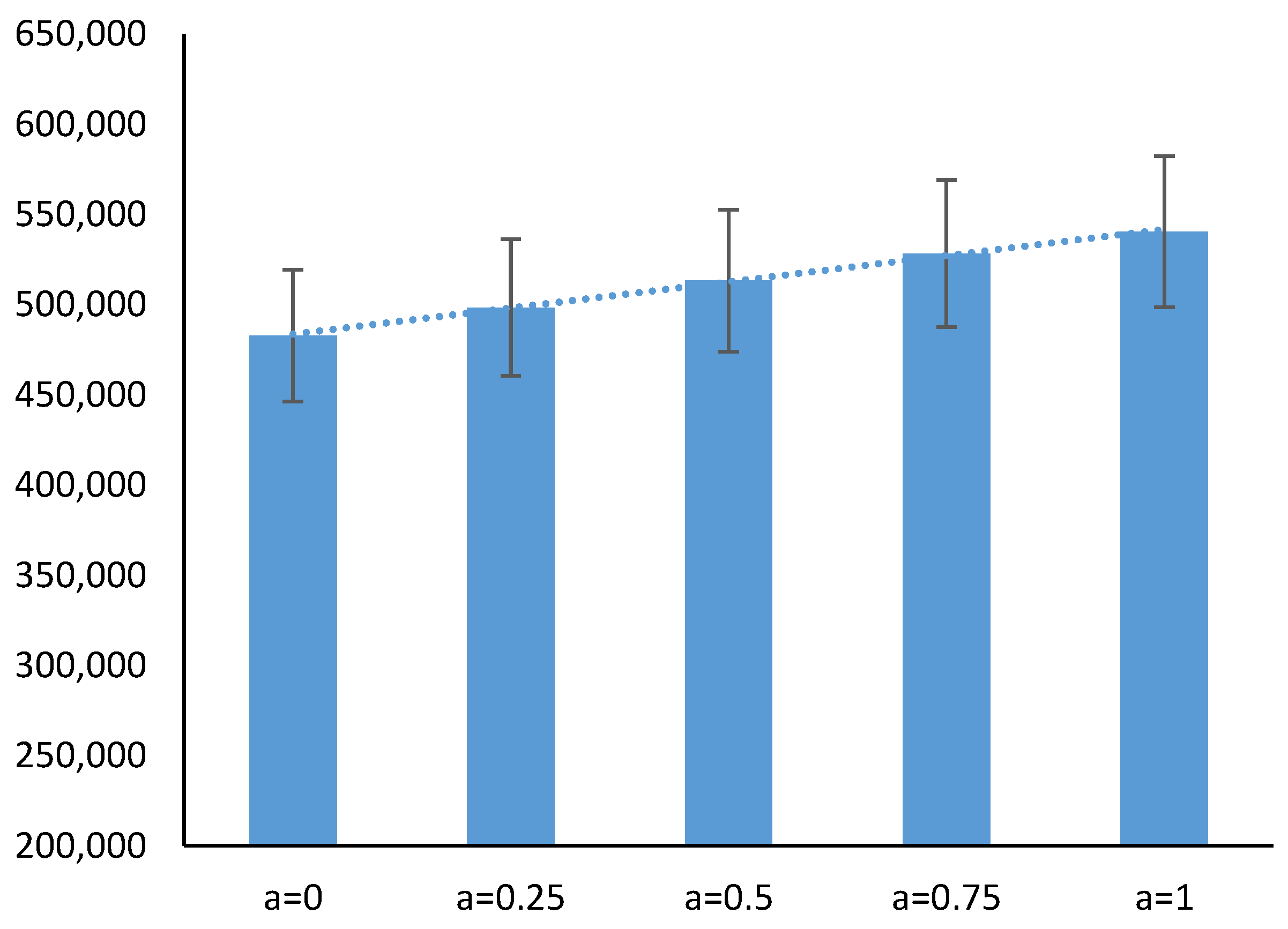
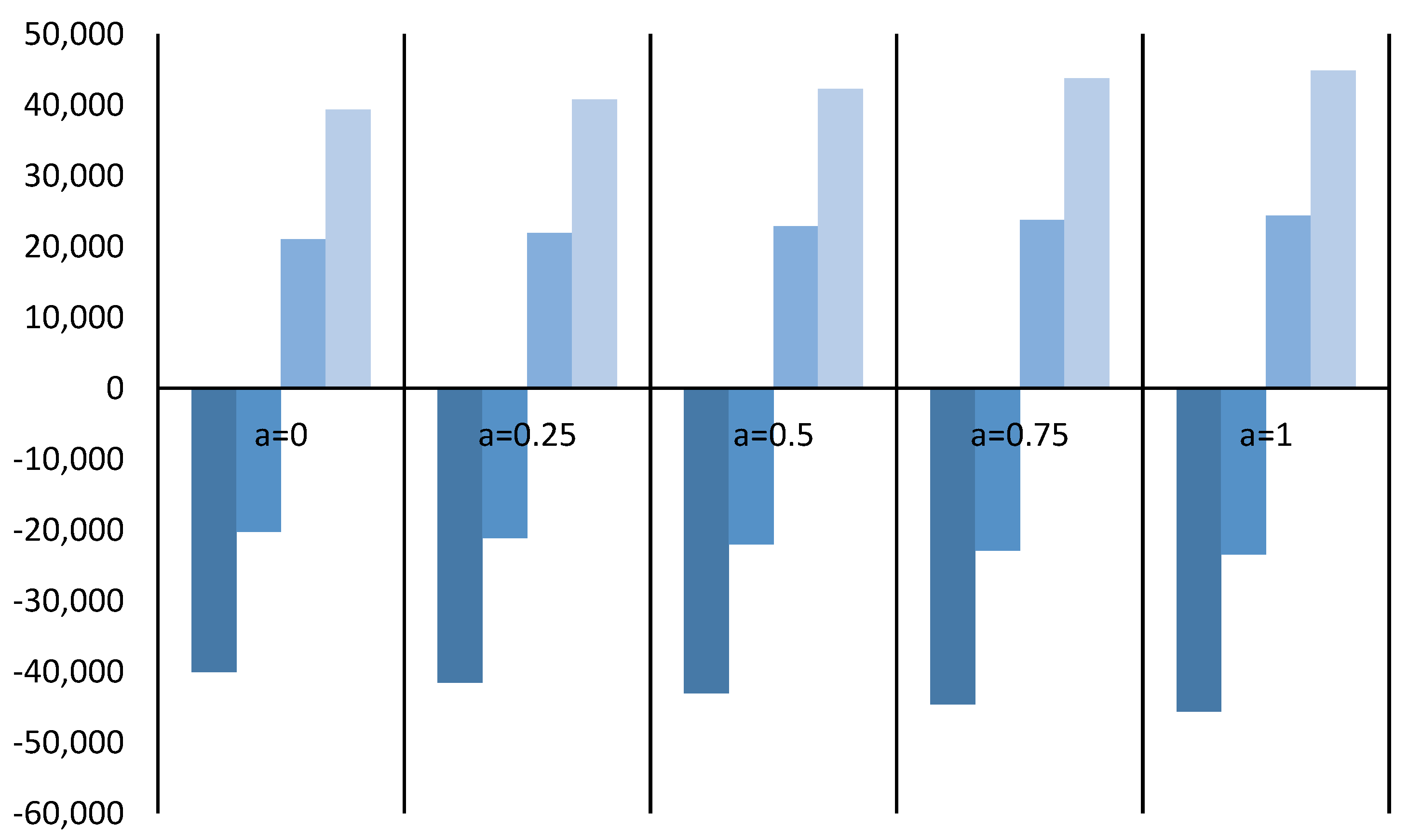
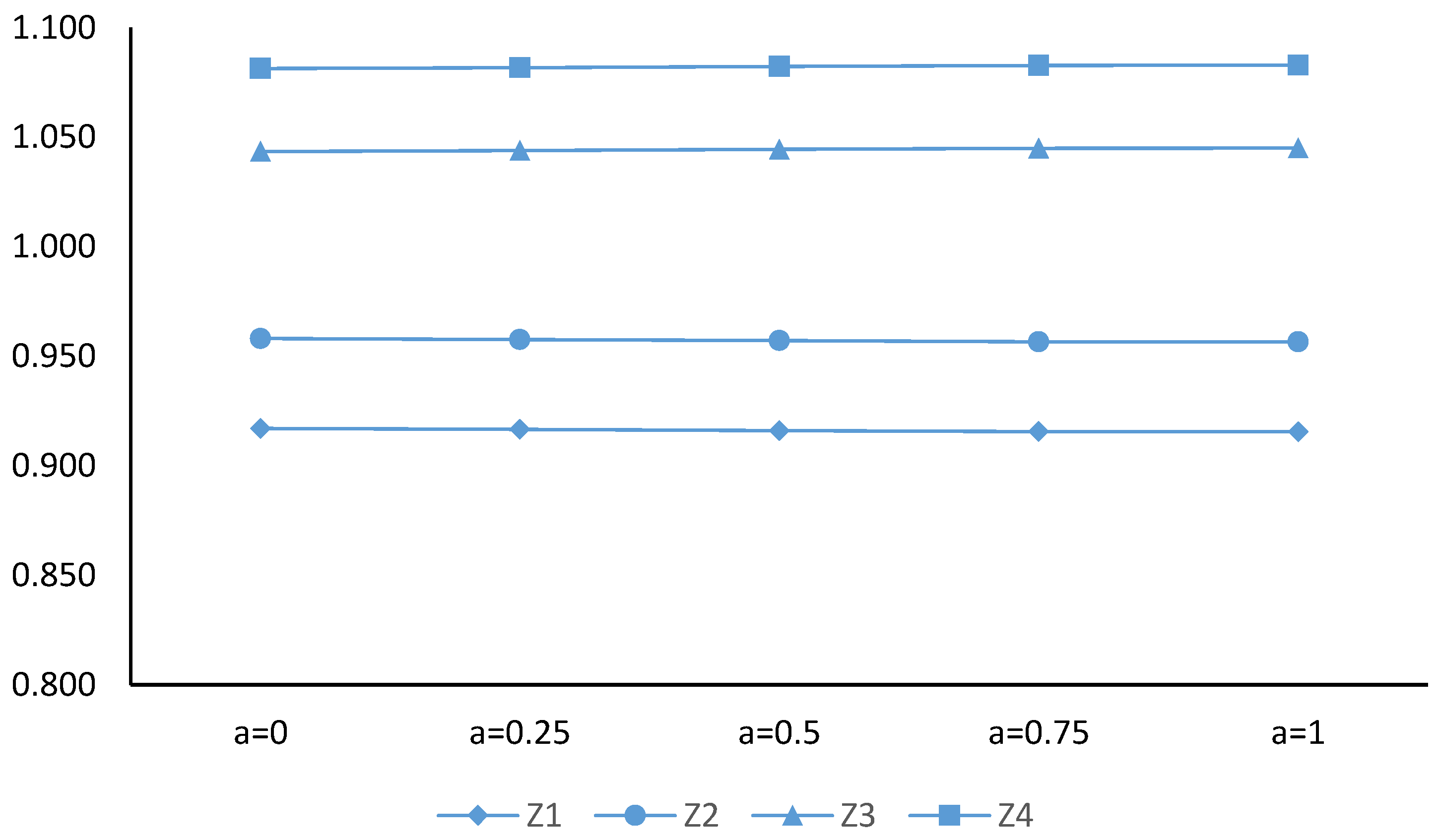
Table 4 lists the predicted entire advantages for each end-user of Xiamen city based on the application of the bi-objective pseudo interval T2 linear programming method with different acceptance degrees. The results exhibit that the total profit of water consumption is calculated to be (442,784, 462,602.6, 503,821.3, 522,116.7) × 106 CNY with acceptance degree = 0. At acceptance degree = 0.75, which is the most common case for FSs, the total profit is estimated as (483,695.5, 505,357.3, 552,043.6, 572,003.8) × 106 CNY for the next 15 years for Xiamen. Figure 4, which is plotted based on Table 4, shows that the higher acceptance degrees match the higher system profits, suggesting that the DMs could receive total profits that are dependent on the a degree. The result data apparently contain four points from Z1 to Z4, which correspond to four points of a single-interval T2 FS. The findings clearly show the advantage in relation to the real-world problem of water systems. The flexibility of the decision process is improved by the use of the interval T2 FS rather than using two interval boundaries. The comparison of the average and standard deviation of the acceptance degrees, which is illustrated in Figure 5 and Figure 6, exhibits the reliability and stability of the results of the optimal value. The results also indicate that the profit value can be closer to (491,303.5, 536,161.5) × 106 CNY with a lower limit of 470,247.9 × 106 CNY and upper limit of 555,563.4 × 106 CNY, for example, when the acceptance degree = 0.5. According to the analysis method of the effects of the uncertainty degree, the advantages presented in Figure 7 show that the lowest and highest uncertain degree that can contribute to an effective solution are less than 4.34% and no more than 8.29%, respectively. Correspondingly, the solutions demonstrate that the interval T2 FSs can really reflect the uncertainties.

Table 4.
Water profit for different acceptance degrees (106 CYN).
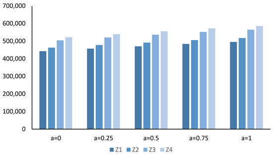
Figure 4.
The total profit over the planning horizon with acceptance degrees.

Figure 5.
The average value of total profit with standard deviations.
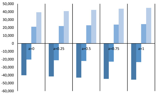
Figure 6.
The average difference for each acceptance degrees.
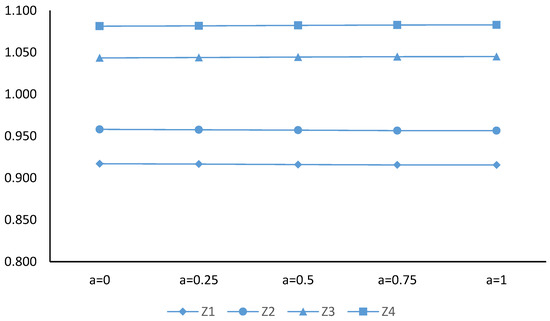
Figure 7.
The uncertain degree of benefit results.
4.2. Water Demands of End-Users
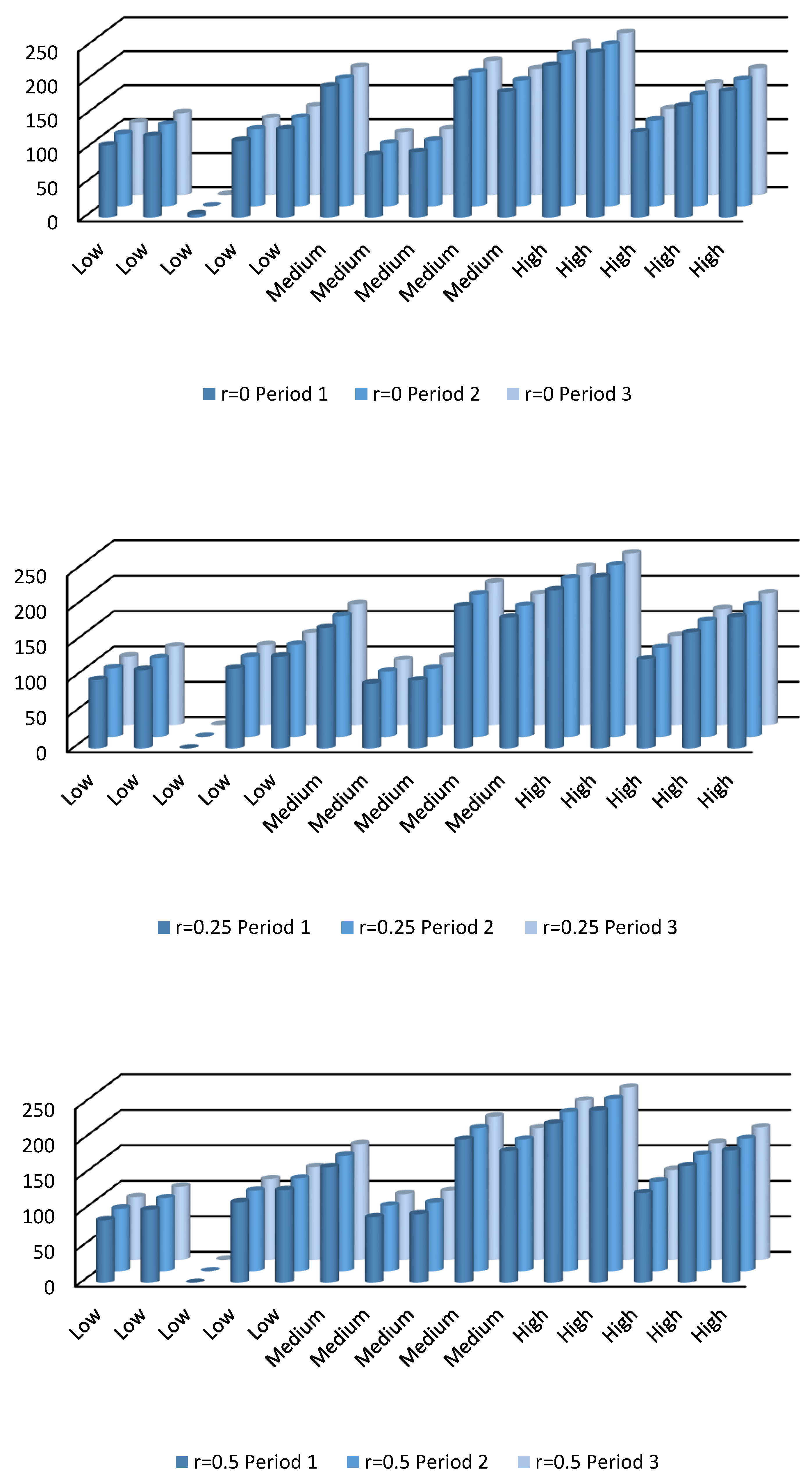
Table 5 lists the water supply quantity for industrial, agricultural, and municipal users at different acceptance degrees. The result shows the required water consumption, which is expected to significantly increase because of the rapid economic activities in the three five-year planning periods. From the perspective of the water level, when the water supply is high, there is a fluctuation in the water demand of the information technology industry in both periods 2 and 3. The water demand of the information technology industry is (223.1, 218, 218, 218, 218) × 106 cubic meters in the second five-year period, and it remains the same in the third five-year period. The results indicate that the DMs can achieve different optimal solutions by choosing different acceptance degrees according to their risk preference. The group of results indicates that such an industry has certain risk preferences for consuming water, which implies that the information technology factories face higher water treatment costs than other industries. This group of results also clarifies that the water volume remains at 223.1 × 10⁶ cubic meters only in the case of zero acceptance degree; it is not constant at other acceptance degrees, including 0.25, 0.5, 0.75, and 1. This trend suggests that this category of industry requires the necessary wastewater treatment to significantly reduce the risk preferences.

Table 5.
Water demands for users under acceptance degrees (106 m3).
When the water level is medium, the results of the petrochemical and biotechnology industries include the results of the interval T2 FSs, which can be dealt with the acceptance degrees by the DMs. The results reveal that there is (230.6, 257.4, 267.8, 278.2, 288.7) × 106 cubic meters of water consumption by the petrochemical industry over the three planning periods, respectively. This indicates that this industry achieves a certain balance by controlling the water quality, water recycling, and wastewater treatment requirements with a relatively medium water supply. By applying a 0.5 acceptance degree, DMs can obtain the optimal solution of 267.8 × 10⁶ cubic meters, which is the common selected result with the fuzzy theory and it largely enhances the flexibility of decision-making. In the biotechnology industry, the water supply is stable in the first period at all acceptance degrees; however, during the second and third planning periods, the demand water is (218.1, 213, 213, 213, 213) × 106 cubic meters. This demand of water implies that the DMs can sufficiently consider the different acceptance degrees when the fuzzy constraints can be violated. It also clearly shows that the starting data of this set of solution is larger than the ending segment data, which implies that the different water volumes correspond to different acceptance degrees. For example, 218.1× 10⁶ cubic meters water is at acceptance degree = zero, which corresponds to a higher system violation risk. At other acceptance degrees, 213 × 106 cubic meters water is allocated to this industry regardless of the period. The lower quantity of water indicates that there may be a water consumption risk owing to the increasing cost of water treatment, which is very good for the local ecosystem as it is saving the water and reducing the waste of water resources.
When the water level is low, the risk of violation of the fuzzy constraints could increase and be affected by the uncertain results of the water supply. The petrochemical, information technology, and machinery industries are individually allocated water supply of (291.2, 302.5, 314.1, 325.5, 337) × 106 cubic meters, (317.1, 328.2, 339.3, 350.4, 361.5) × 106 cubic meters, and (491.2, 496.3, 496.3, 496.3, 496.3) × 106 cubic meters, respectively. Owing to the high profit of the machinery industry in Xiamen city, its water consumption is also gradually increased with a lower risk of constraint violation, and it maintains a maximum water supply during the second and third periods. The FS of the results is mostly obtained from the wastewater treatment cost with water recycling activities, which help improve the local environment. Under the constraints of the local environmental regulations. For example, the treatment rate of recycling water, the risk of water consumption would be particularly taken by the petrochemical and information technology factories, and the balance of profit will increase the usage by the industries.
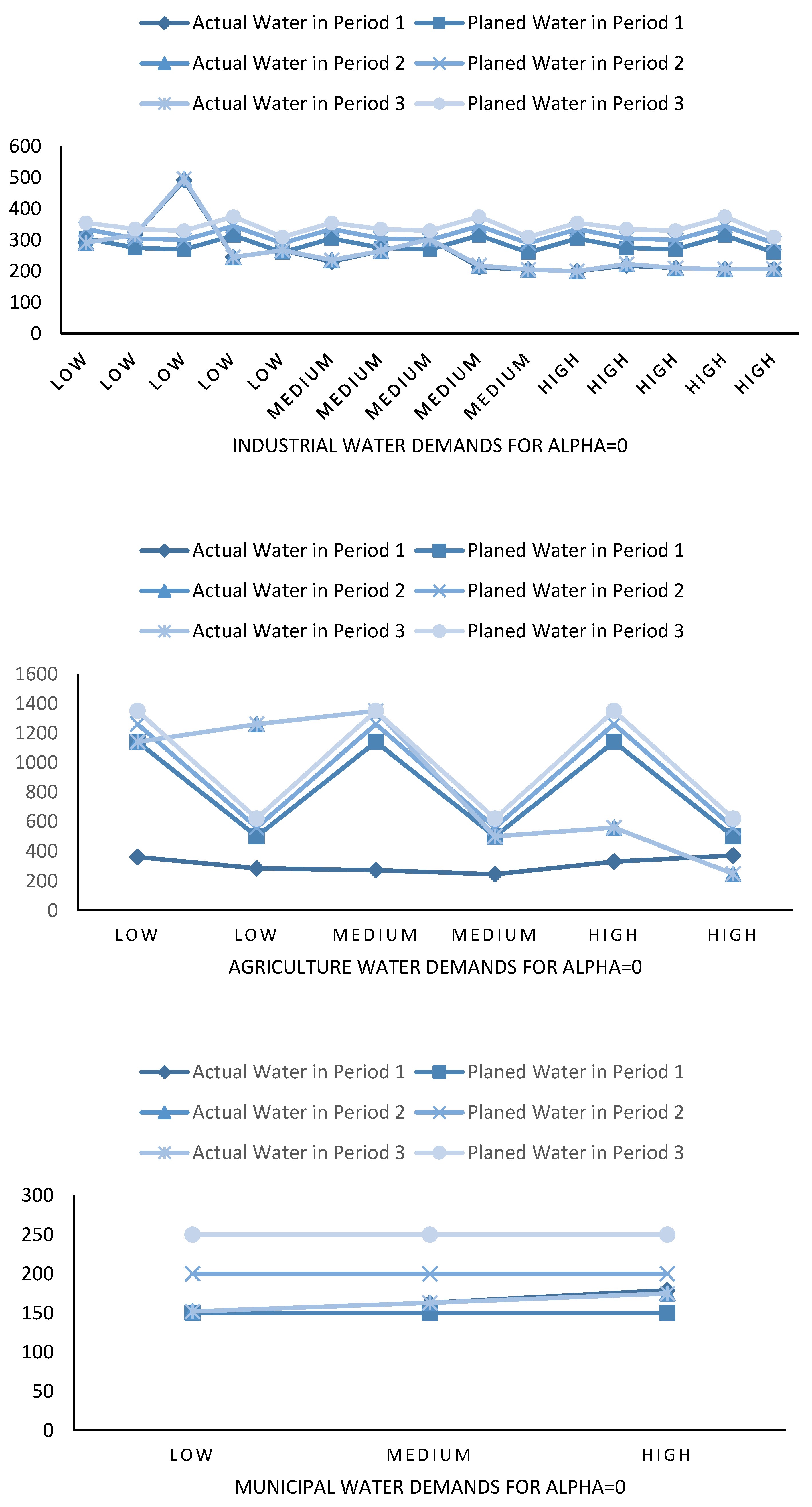
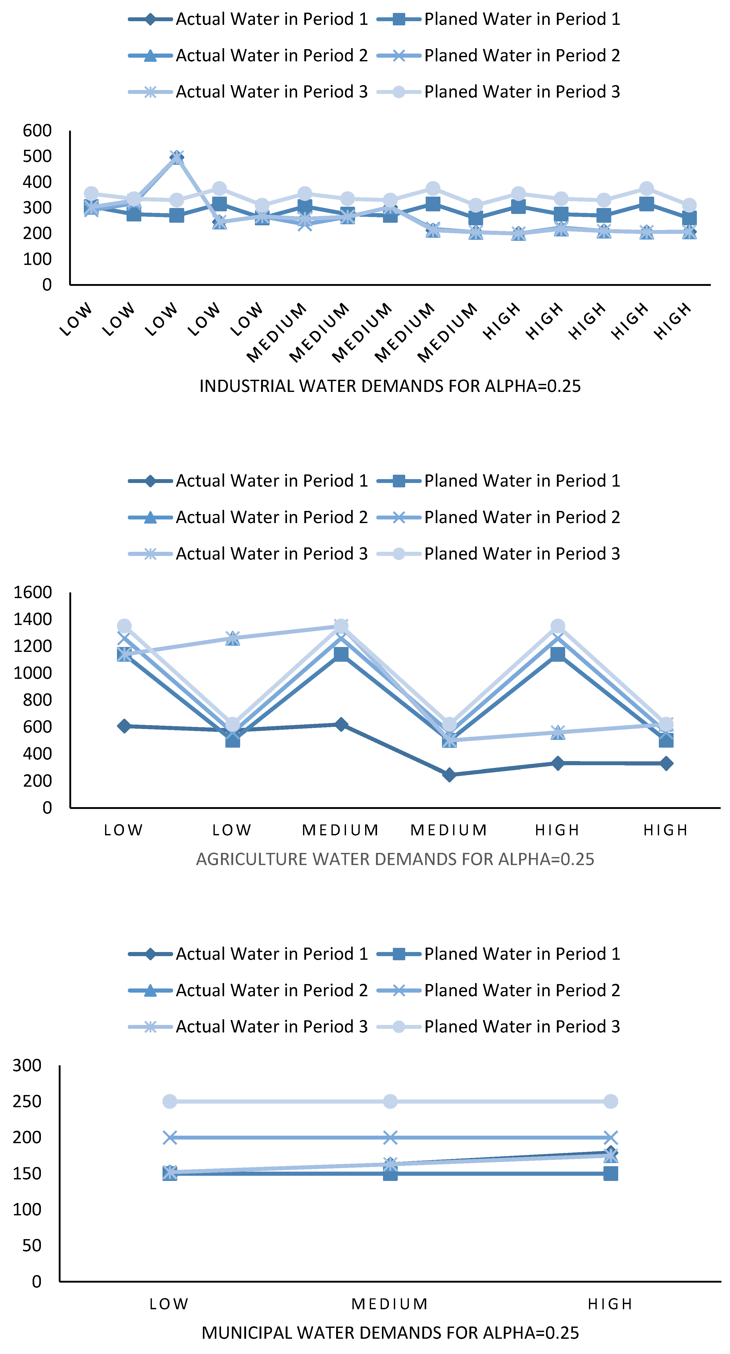
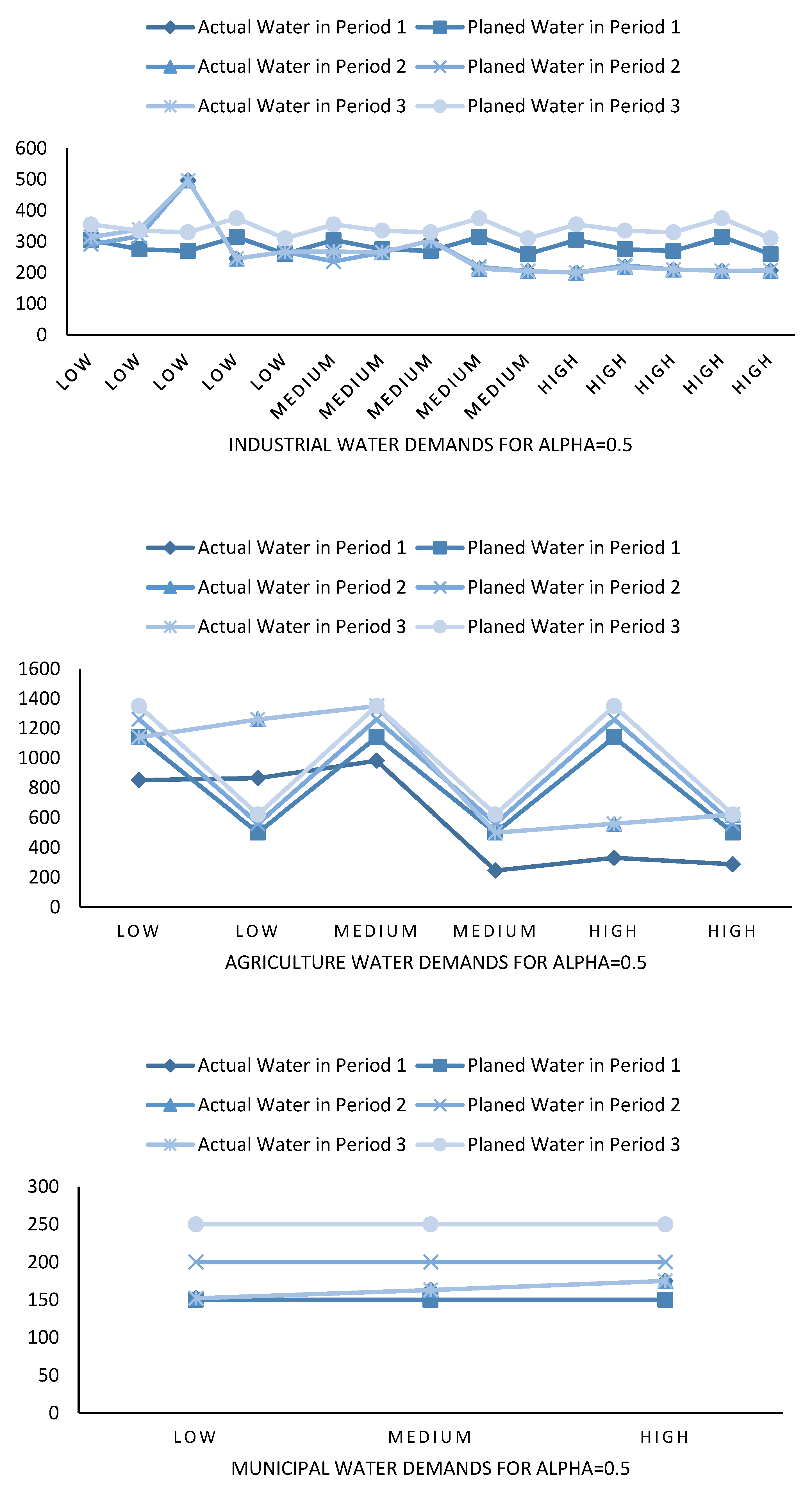
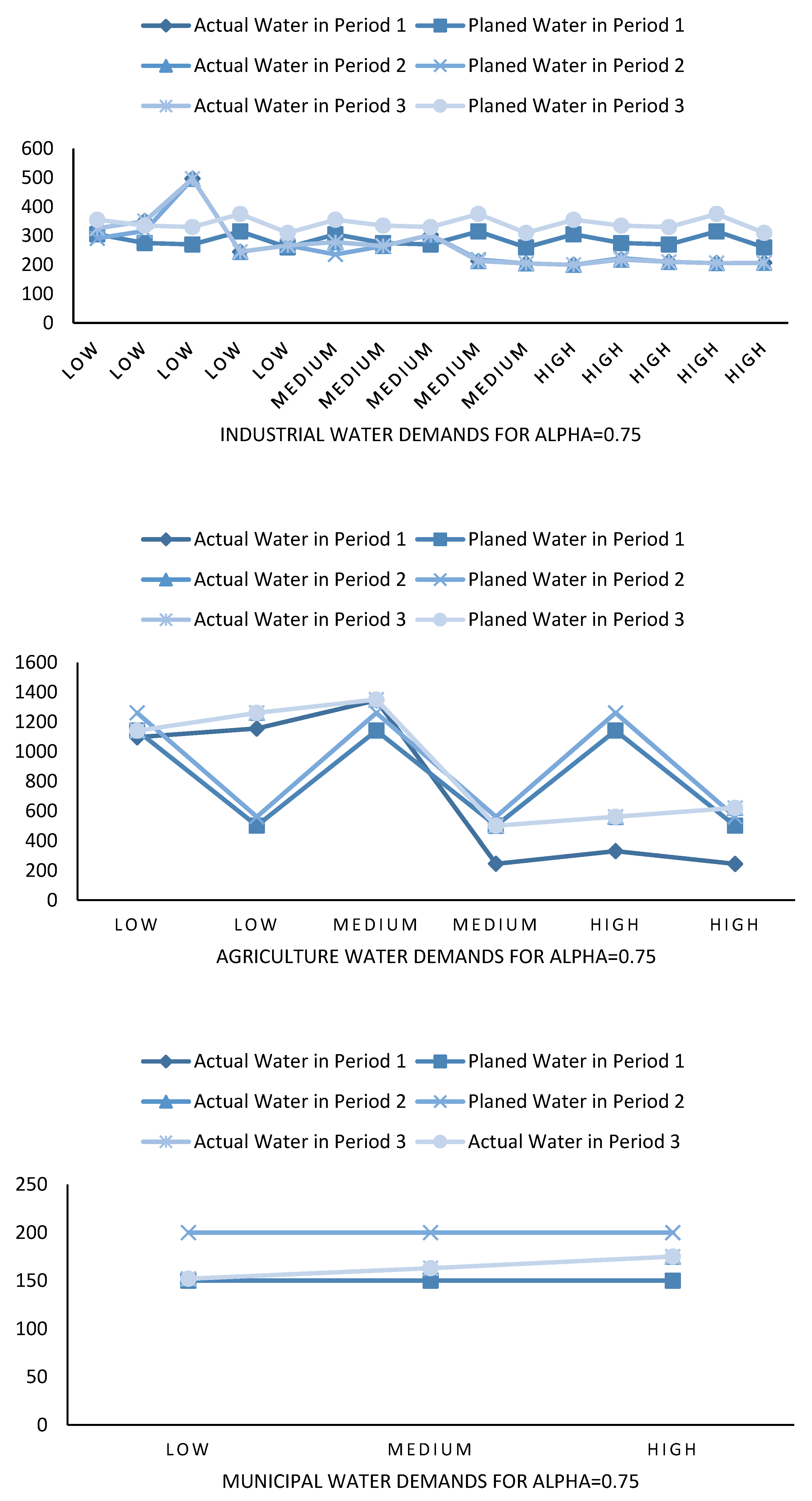
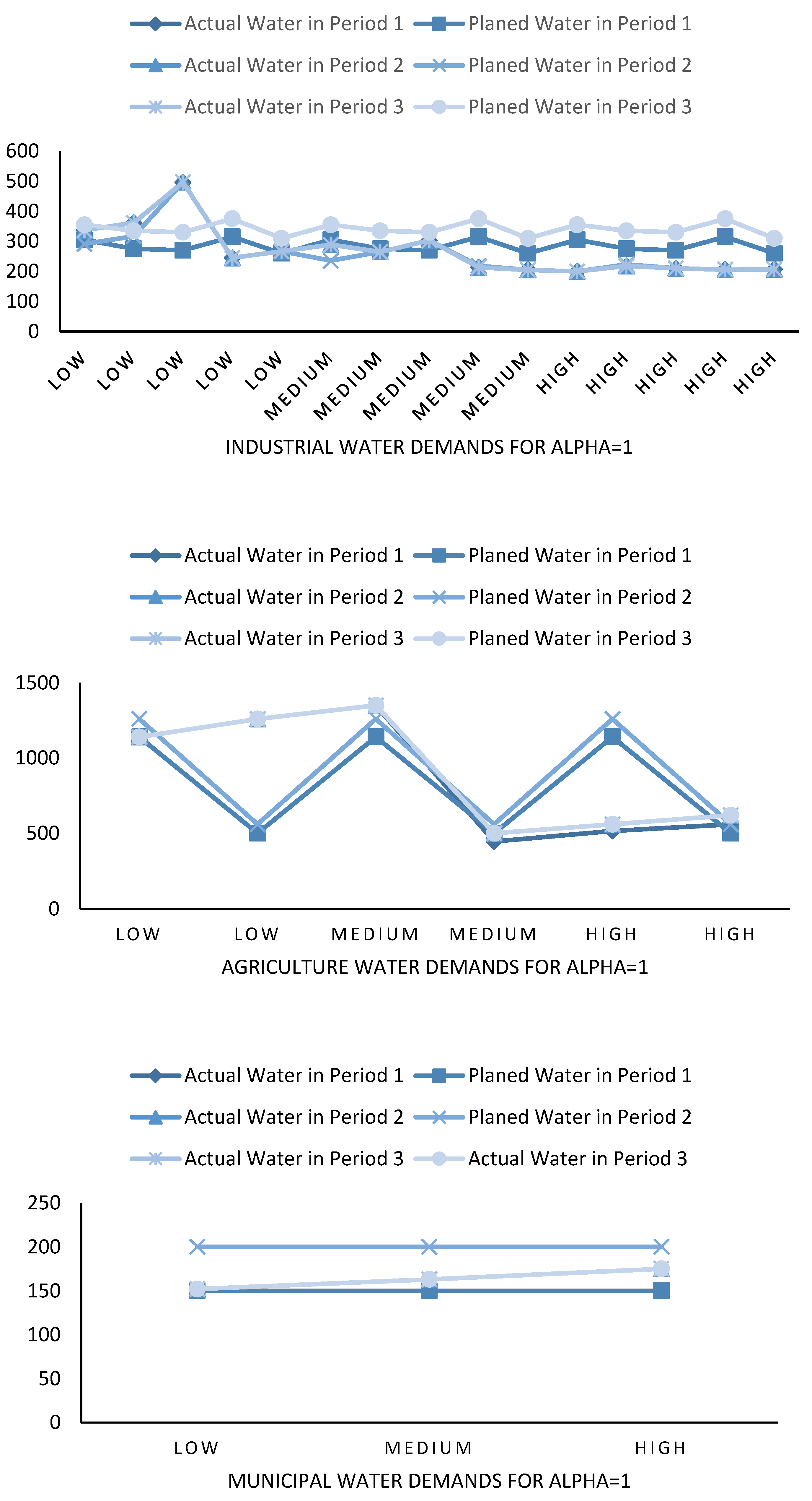
A comparison of the actual water consumption and planned water supply in the three periods is shown in Figure 8. The results indicate that the water demand of all the industries at Xiamen city is estimated to be less than the planned water volumes. This confirms that the cost of water treatment, including fresh water and wastewater treatment, is an effective tool for reducing the water supply of factories. This implies that a higher usage of water is associated with more responsibility. The remaining amount of water can be returned for usage by the municipal bodies, which would reduce the daily living cost of the population in this city. In this figure, for example, when the DMs take 0.5 acceptance degree for the entire water system, the water demand by agriculture is obviously higher than the planned water volume, except for the water usage in the first period. The first period of this water model is based on the assumptions of the beginning year. However, in the second five-year period, the water demand increases to the volume of planned water. This is owing to the lower cost of water supply. For agricultural water, individual water treatment and recycling of water are not required. Therefore, the quantity of water that can be supplied to this sector is naturally increased. Moreover, the reduction in the industrial water demand leads to a lower cost of sharing of the excess water. Similar to an industrial user, the municipal water supply is much lower than planned. This is not only caused by the level of natural water but also by the cost of the wastewater treatment. This will encourage citizens in this area to save more water, which will definitely have a positive effect on the population development. However, the results of water supply would be changed with the violation of the constraints. Consequently, the DMs should take more steps to evaluate the system risk and make a practical decision based on the regulation of the local environment. To complete such requirements, it is a remarkable feature of method under different acceptance degrees.
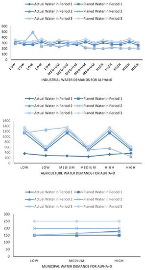
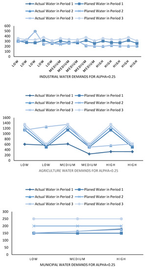
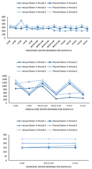
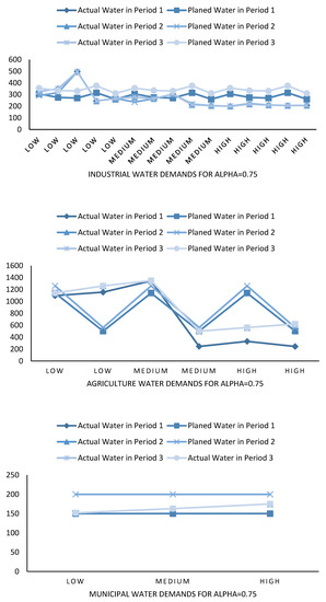
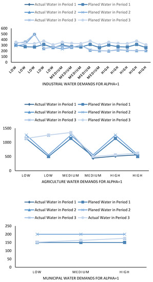
Figure 8.
Comparison of actual water and planned water under acceptance degrees.
This study also discussed the effect of water shortage on each end-user at different acceptance degrees and water levels. The variations in water shortage are mostly caused by the water quality control, water treatment cost, and water level. Figure 9 as an example shows that the industrial users contribute the most to water shortage at each water level, particularly at a high-water level. This implies that although the industrial users are high-profit producers, they also encounter a high-water cost, and so, only reduce the water consumption to reduce the costs and increase the profits for each unit. The water that is planned for the industrial users is supplied to the agricultural and municipal users. Therefore, according to the modeling results, agricultural users have the least water in any period or at any acceptance degree. The agricultural users only face a shortage of water in period 1, but have a sufficient supply in periods 2 and 3. For the municipal users, the water shortage is 37 × 106 cubic meters and 75 × 106 cubic meters, which is common at medium and high water levels. However, at a low water-level, a municipal user is confronted with water shortage. This is because of the high cost of purchasing water from other cities. Additionally, major results of water shortage at the acceptance degree of 0.5 are presented in Table 6, which includes the water shortage for three types of users: industrial, agricultural, and municipal consumers. Compared with the other results at different acceptance degrees, the main difference is in the supply of water to the industrial users. Specifically, with a higher acceptance degree, a smaller quantity of water is supplied to the industrial users, except the machinery industry, which is accompanied by a large profit of water usage. This scenario is also consistent with the actual requirement of the local area.
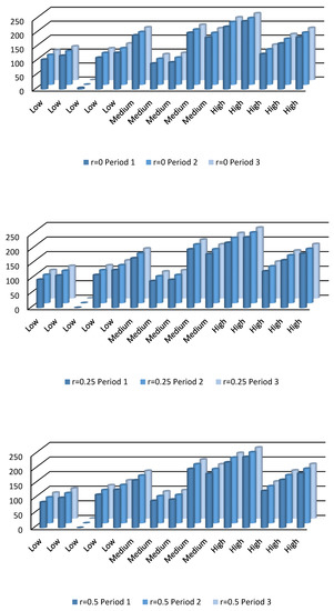
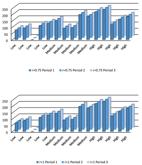
Figure 9.
Water shortage for industrial users under different acceptance degrees.

Table 6.
Water shortage under 0.5 acceptance degree (106 m3).
4.3. Recycled Water Demands
Recycled water is an important part of water consumption and supply. In this case, it accounts for one-third of the industrial water usage. Table 7 presents the details of the recycled water for each industrial user at different acceptance degrees. It shows that when the acceptance degree is 0.5, the petrochemical industry requires 97.21333 × 10⁶, 106.9806 × 10⁶, and 141.25 × 10⁶ cubic meters water from period 1 to period 3, respectively. This accounts for 47.4% demand of the water supply at a medium water level. Because of the lower cost of recycling water, it should be the important part of this city. Effective usage of recycled water by this modeling results is a major strategy for reducing the industrial costs. However, for agricultural users, the cost of recycling water is high and the produced recycled water is difficult to collect during the fertilization process. Similarly, for the municipal users, there is a high process fee for recycling water compared to transferring the water from industrial users. However, the recycled water for either municipal or agricultural users should be increased for the purpose of flushing toilets and landscape water application. For this, the processing costs are very low if the recycled water rate is further increased by the industrial users. Overall, in this modeling process of the Xiamen water system, there are many uncertainties, which can cause a conflict between the water supply and treatment cost. The right use of this new uncertain method is the main route for resolving such issues. However, this modeling process has limited calculation power, because of which many factors or indices, such as population factors, are still not considered in the simulation, which will be further revised in future modeling.

Table 7.
Recycled water usage for industrial users under acceptance degrees (106 m3).
4.4. Comparative Analysis
By comparison of previous methods, the advantages of developed method can easily find that the transformation process of previous methods can cause great distortion of uncertain information. Some methods linked possibility distribution or dynamical features [39] can make too many objective functions or/and constraints in the actual model, which increased the calculation force and complexity of the solution process. For example, the dynamical modeling method [40,41] converts the multiple-dimensions regulation into a complex fuzzy characteristic. Similarly, some methods referred to degree of fuzzy constraints but missed to considered the dissatisfaction degree of fuzzy sets. Some fuzzy methods used triangular fuzzy sets/number to instead of trapezoidal membership. These methods are one-sided and do not represent the majority of fuzzy situations. To cover such disadvantages of previous works, the focus of this demonstrated approach is a proposed novel programming method to solve general fuzzy linear programming issues for water resources management considering the fuzzy acceptance degree and it may be violated under realistic conditions. With the order relation of general fuzzy sets, a new bi-objective linear program is developed. The order relationship for proposed approach is defined through the interval expectation. Because of its order relation of interval T2 fuzzy sets, the general fuzzy linear programming is transformed into interval objective programming method [31]. Thereby, this method can be further transformed into a bi-objective LP by employing the ranking relation. Therefore, this developed method contains the advantages of mathematical rigor and logic in combination with uncertain programming theories.
5. Conclusions
This study proposed a novel bi-objective interval T2 programming model, in which the objective function and technological coefficients resources are all fuzzy sets, for the water planning of Xiamen city. Optimal solutions were provided for three water users by the modeling process, in which the uncertain impact factors were included and quantified. Based on the given order relationship of the interval fuzzy sets, this interval T2 linear programming model was transformed into a bi-objective linear programming model and solved by a goal programming approach. The method enhanced the flexibility of the optimal processes and offers decision-makers a better support with realist scenarios, where this violation of the constraints. This was achieved by fully considering the acceptance degree of the local environmental requirements of water treatment. In addition, recycled water usages were presented for industrial users at each acceptance degree. Moreover, the comparison between actual supplied water and planned water was used to represent the real water distribution of Xiamen city and also illustrate the advantage of the development algorithm.
This was this first application of a bi-objective pseudo-interval T2 linear programming method to a real water system in Xiamen, China. The solution obtained from this novel model indicates that (a) the quantify of water supplied to the industrial users in this region needed to be reduced owing to the water processing cost; (b) local factories should increase the quantity water supply from recycled water; (c) municipal and agricultural users should get priority for water supply; (d) with the increase in the acceptance degree, the quantity of recycled water should be increased, i.e., to increase the recycling water by industrial factories should reduce the risk of insufficient water supply in this area. This study also developed a new method for a pseudo-interval type-2 fuzzy set programming. By the application of the ranking order relation of the pre-defined interval expectation method, this model can transform into a bi-objective linear program. The solutions from this model completely exhibited the acceptance degree of the system, which significantly increases the flexibility of the decision process and improves the optimal results of real engineering problems. The highlights of the proposed method can be concluded as follows: (1) propose a new reliable arithmetical model for water systems; (2) process uncertainty based on α-cuts and α-planes (z-slices) algorisms; (3) tackle type-2 fuzzy sets without loss of generality; (3) refine decision spaces for the linear programming under uncertainty; (4) provide decision makers with better options for the Southern Min area of China. However, one correction was required in the future studies. A comprehensive systematic water model with systematic constraints including population and more economical factors should be added to the modeling process in a future study. Thus, with the high complexity of the uncertainties, the advantages of the abilities of this method, including the objective functions and technological and recourse coefficients in the linear programming, could be better displayed.
Author Contributions
H.F. and L.J. are the two main writers of this manuscript; L.J. developed the new approach of this paper. Y.K. was responsible for the quality control of this manuscript. J.L. was responsible for the data collection; G.H. was responsible for development of the interval theory.
Acknowledgments
This research was supported by the Natural Science Foundation of Fujian Province (Grant No. 2018J01527) and Fujian Science and Technology Guiding Project (grant no. 2018Y0079). Key Laboratory of Environmental biotechnology, Fujian Province University. The authors are grateful to the editors and the anonymous reviewers for their insightful comments and suggestions.
Conflicts of Interest
The authors declare that there is no conflict of interest for publication of this paper.
Abbreviations
The indices in Equations (14a–m) represent the following:
| Notation | |
| i | five subcategories of industrial classification, namely, petrochemical industry, information technology industry, machinery industry, biotechnology industry, and marine technology industry; |
| a | two categories of agricultural classification, namely, crop agriculture and animal husbandry; |
| t | three five-year plans of China; |
| h | water inflow level (h = 1, 2, and 3 for low, medium, and high level, respectively); |
| industrial raw water volume, m3; | |
| industrial reuse water volume, m3; | |
| industrial unit water profit, yuan/m3; | |
| agricultural raw water volume, m3; | |
| agricultural unit water profit, yuan/m3; | |
| municipal water consumption, m3; | |
| municipal reuse water volume, m3; | |
| municipal unit water profit, yuan/m3; | |
| water shortage for the industrial categories, m3; | |
| unit reduction in the net benefit when the water supply target is not delivered to the industrial categories, yuan/m3; | |
| water shortage for the agricultural categories, m3; | |
| reduction in the net benefit when the water supply target is not delivered to the agricultural categories, yuan/m3; | |
| water shortage for the municipal bodies, m3; | |
| reduction in the net benefit when the water supply target is not delivered to the municipal bodies, yuan/m3; | |
| industrial reuse water unit water supply cost, yuan/m3; | |
| municipal reuse water cost, yuan/m3; | |
| industrial sewage treatment cost, yuan/m3; | |
| industrial sewage production rate; | |
| municipal sewage treatment cost, yuan/m3; | |
| municipal sewage production rate; | |
| municipal water consumption, m3; | |
| total water available in the area, 104 m3; | |
| amount of water demand for the industrial categories, m3; | |
| amount of water demand for the agricultural categories, m3; | |
| amount of water demand for the municipal bodies, m3; | |
| reduced rainfall, 108 m3; | |
| industrial wastewater discharge rate; | |
| municipal wastewater discharge rate; | |
| capacity of the sewage treatment, m3 |
References
- Huang, Y.; Chen, X.; Li, Y.; Willems, P.; Liu, T. Integrated modeling system for water resources management of Tarim River Basin. Environ. Eng. Sci. 2010, 27, 255–269. [Google Scholar] [CrossRef]
- Jin, L.; Huang, G.; Fan, Y.; Nie, X.; Cheng, G. A hybrid dynamic dual interval programming for irrigation water allocation under uncertainty. Water Resour. Manag. 2012, 26, 1183–1200. [Google Scholar] [CrossRef]
- Li, Y.; Huang, G.; Nie, S. An interval-parameter multi-stage stochastic programming model for water resources management under uncertainty. Adv. Water Resour. 2006, 29, 776–789. [Google Scholar] [CrossRef]
- Li, Y.; Huang, G.H.; Huang, Y.; Zhou, H. A multistage fuzzy-stochastic programming model for supporting sustainable water-resources allocation and management. Environ. Model. Softw. 2009, 24, 786–797. [Google Scholar] [CrossRef]
- Luo, B.; Maqsood, I.; Yin, Y.; Huang, G.; Cohen, S. Adaption to climate change through water trading under uncertainty-An inexact two-stage nonlinear programming approach. J. Environ. Inf. 2015, 2, 58–68. [Google Scholar] [CrossRef]
- Nematian, J. An extended two-stage stochastic programming approach for water resources management under uncertainty. J. Environ. Inform. 2016, 27. [Google Scholar] [CrossRef]
- Thissen, W.; Kwakkel, J.; Mens, M.; Van der Sluijs, J.; Stemberger, S.; Wardekker, A.; Wildschut, D. Dealing with uncertainties in fresh water supply: Experiences in the Netherlands. Water Resour. Manag. 2017, 31, 703–725. [Google Scholar] [CrossRef]
- Liu, D.; Liu, W.; Fu, Q.; Zhang, Y.; Li, T.; Imran, K.M.; Abrar, F.M. Two-stage multi-water sources allocation model in regional water resources management under uncertainty. Water Resour. Manag. 2017, 31, 3607–3625. [Google Scholar] [CrossRef]
- Parker, G.G.; Ferguson, G.E.; Love, S.K. Water Resources of Southeastern Florida, with Special Reference to Geology and Ground Water of the Miami Area; U.S. G.P.O.: Washington, WA, USA, 1955.
- Abdulbaki, D.; Al-Hindi, M.; Yassine, A.; Najm, M.A. An optimization model for the allocation of water resources. J. Clean. Prod. 2017, 164, 994–1006. [Google Scholar] [CrossRef]
- Celik, E.; Gul, M.; Aydin, N.; Gumus, A.T.; Guneri, A.F. A comprehensive review of multi criteria decision making approaches based on interval type-2 fuzzy sets. Knowl.-Based Syst. 2015, 85, 329–341. [Google Scholar] [CrossRef]
- Ahmad, A.; El-Shafie, A.; Razali, S.F.M.; Mohamad, Z.S. Reservoir optimization in water resources: A review. Water Resour. Manag. 2014, 28, 3391–3405. [Google Scholar] [CrossRef]
- Daghighi, A.; Nahvi, A.; Kim, U. Optimal cultivation pattern to increase revenue and reduce water use: Application of linear programming to arjan plain in Fars province. Agriculture 2017, 7, 73. [Google Scholar] [CrossRef]
- Miao, D.; Huang, W.; Li, Y.; Yang, Z. Planning water resources systems under uncertainty using an interval-fuzzy de novo programming method. J. Environ. Inform. 2014, 24. [Google Scholar] [CrossRef]
- Wang, S.; Huang, G. A multi-level Taguchi-factorial two-stage stochastic programming approach for characterization of parameter uncertainties and their interactions: An application to water resources management. Eur. J. Oper. Res. 2015, 240, 572–581. [Google Scholar] [CrossRef]
- Chen, Y.; He, L.; Lu, H.; Li, J.; Ren, L. Planning for regional water system sustainability through water resources security assessment under uncertainties. Water Resour. Manag. 2018, 32, 3135–3153. [Google Scholar] [CrossRef]
- Dai, R.; Charkhgard, H. A two-stage approach for bi-objective integer linear programming. Oper. Res. Lett. 2018, 46, 81–87. [Google Scholar] [CrossRef]
- Charkhgard, H.; Eshragh, A. Best subset selection in linear regression via bi-objective mixed integer linear programming. arXiv, 2018; arXiv:1804.07935. [Google Scholar]
- Saghand, P.G.; Charkhgard, H.; Kwon, C. A branch-and-bound algorithm for a class of mixed integer linear maximum multiplicative programs: A bi-objective optimization approach. Comput. Oper. Res. 2018, 101, 263–274. [Google Scholar] [CrossRef]
- Naderi, M.; Pishvaee, M. Robust bi-objective macroscopic municipal water supply network redesign and rehabilitation. Water Resour. Manag. 2017, 31, 2689–2711. [Google Scholar] [CrossRef]
- Irawan, C.A.; Jones, D.; Ouelhadj, D. Bi-objective optimisation model for installation scheduling in offshore wind farms. Comput. Oper. Res. 2017, 78, 393–407. [Google Scholar] [CrossRef]
- Belmonte, B.A.; Benjamin, M.F.D.; Tan, R.R. Bi-objective optimization of biochar-based carbon management networks. J. Clean. Prod. 2018, 188, 911–920. [Google Scholar] [CrossRef]
- Vahdani, B.; Tavakkoli-Moghaddam, R.; Jolai, F.; Baboli, A. Reliable design of a closed loop supply chain network under uncertainty: An interval fuzzy possibilistic chance-constrained model. Eng. Optim. 2013, 45, 745–765. [Google Scholar] [CrossRef]
- Huang, G.H.; Baetz, B.W.; Patry, G.G. A grey fuzzy linear programming approach for municipal solid waste management planning under uncertainty. Civ. Eng. Syst. 1993, 10, 123–146. [Google Scholar] [CrossRef]
- Jin, L.; Huang, G.H.; Wang, L.; Wang, X. Robust fully fuzzy programming with fuzzy set ranking method for environmental systems planning under uncertainty. Environ. Eng. Sci. 2013, 30, 280–293. [Google Scholar] [CrossRef]
- Baky, I.A. Fuzzy goal programming algorithm for solving decentralized bi-level multi-objective programming problems. Fuzzy Sets Syst. 2009, 160, 2701–2713. [Google Scholar] [CrossRef]
- Sinha, S. Fuzzy programming approach to multi-level programming problems. Fuzzy Sets Syst. 2003, 136, 189–202. [Google Scholar] [CrossRef]
- Kumar, D.; Rahman, Z.; Chan, F.T. A fuzzy AHP and fuzzy multi-objective linear programming model for order allocation in a sustainable supply chain: A case study. Int. J. Comput. Integr. Manuf. 2017, 30, 535–551. [Google Scholar] [CrossRef]
- Takami, M.A.; Sheikh, R.; Sana, S.S. A hesitant fuzzy set theory based approach for project portfolio selection with interactions under uncertainty. J. Inf. Sci. Eng. 2018, 34, 65–79. [Google Scholar]
- Zadeh, L. Fuzzy sets. Inf. Control 1965, 8, 338–353. [Google Scholar] [CrossRef]
- Huang, G.H. IPWM: An interval parameter water quality management model. Eng. Optim. 1996, 26, 79–103. [Google Scholar] [CrossRef]
- Hu, C.; Kearfott, R.B.; De Korvin, A.; Kreinovich, V. Knowledge Processing with Interval and Soft Computing; Springer: London, UK, 2008; ISBN 978-1-84800-325-5. [Google Scholar]
- Dong, J.Y.; Wan, S.P. A new trapezoidal fuzzy linear programming method considering the acceptance degree of fuzzy constraints violated. Knowl.-Based Syst. 2018, 148, 100–114. [Google Scholar] [CrossRef]
- Ishibuchi, H.; Tanaka, H. Multiobjective programming in optimization of the interval objective function. Eur. J. Oper. Res. 1990, 48, 219–225. [Google Scholar] [CrossRef]
- Karnik, N.N.; Mendel, J.M. Operations on type-2 fuzzy sets. Fuzzy Sets Syst. 2001, 122, 327–348. [Google Scholar] [CrossRef]
- Srinivasan, A.; Geetharamani, G. Linear programming problem with interval type 2 fuzzy coefficients and an interpretation for ITS constraints. J. Appl. Math. 2016, 1, 1–11. [Google Scholar] [CrossRef]
- Jin, L.; Huang, G.; Cong, D.; Fan, Y. A robust inexact joint-optimal α cut interval type-2 fuzzy boundary linear programming (RIJ-IT2FBLP) for energy systems planning under uncertainty. Int. J. Electr. Power Energy Syst. 2014, 56, 19–32. [Google Scholar] [CrossRef]
- Statistical Communique of Xiamen’s City Economic and Social Development Xiamen Statistics Bureau. Available online: http://www.stats-xm.gov.cn/ (accessed on 28 May 2018).
- Kuriqi, A. Simulink application on dynamic modelling of biological wastewater treatment for aerator tank case. Int. J. Sci. Technol. Res. 2014, 3, 69–72. [Google Scholar]
- Kuriqi, A.; Kuriqi, I.; Poci, E. Simulink Programming for Dynamic Modelling of Activated Sludge Process: Aerator and Settler Tank Case. Fresen. Environ. Bull. 2016, 25, 2891. [Google Scholar]
- Zhao, J.; Li, M.; Guo, P.; Zhang, C.; Tan, Q. Agricultural water productivity-oriented water resources allocation based on the coordination of multiple factors. Water 2017, 9, 490. [Google Scholar] [CrossRef]
© 2018 by the authors. Licensee MDPI, Basel, Switzerland. This article is an open access article distributed under the terms and conditions of the Creative Commons Attribution (CC BY) license (http://creativecommons.org/licenses/by/4.0/).

