A Bi-Objective Pseudo-Interval T2 Linear Programming Approach and Its Application to Water Resources Management Under Uncertainty


Abstract
1. Introduction
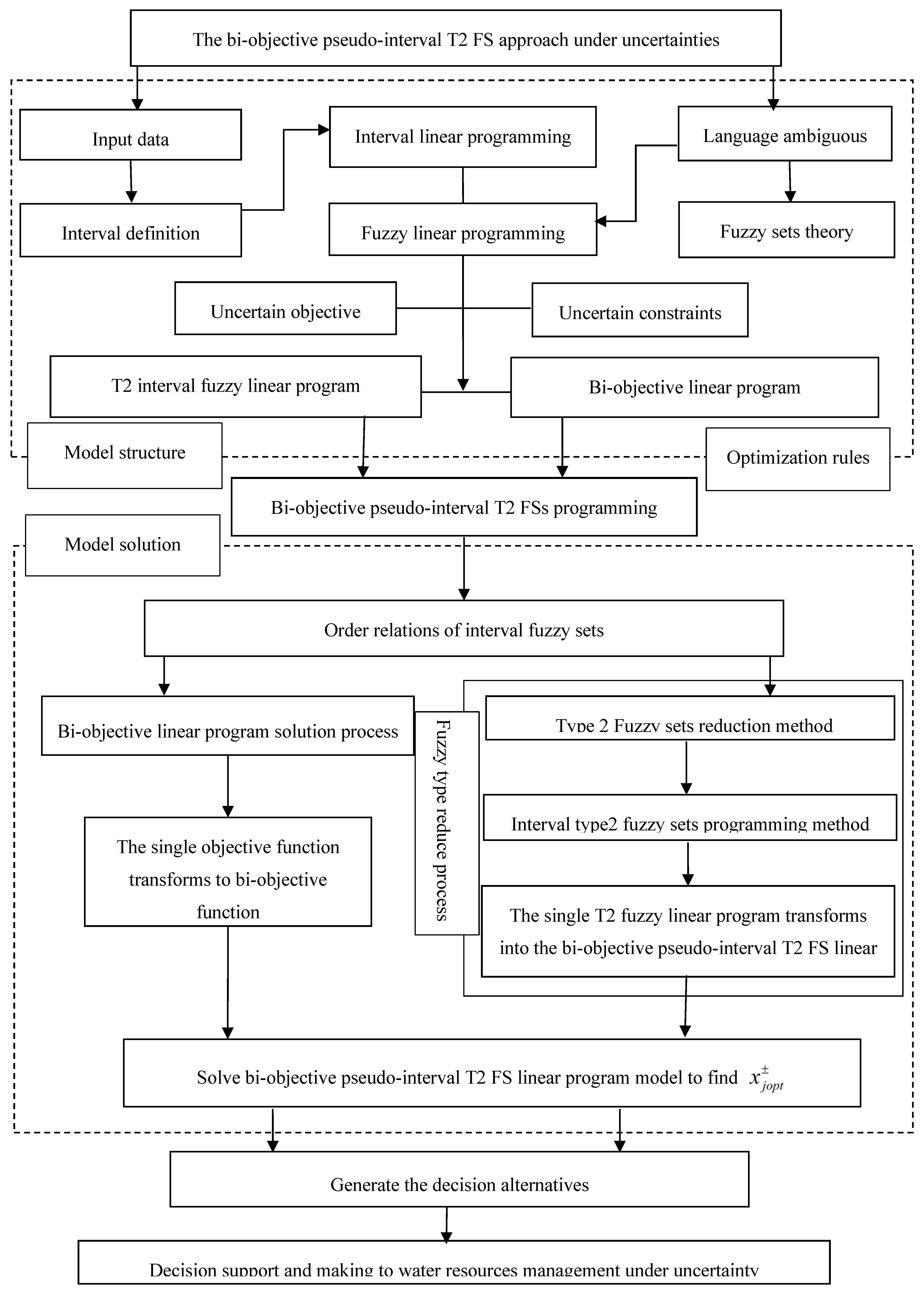
2. Methodology
2.1. Order Relations for Interval Fuzzy Sets
2.2. Bi-Objective Linear Program
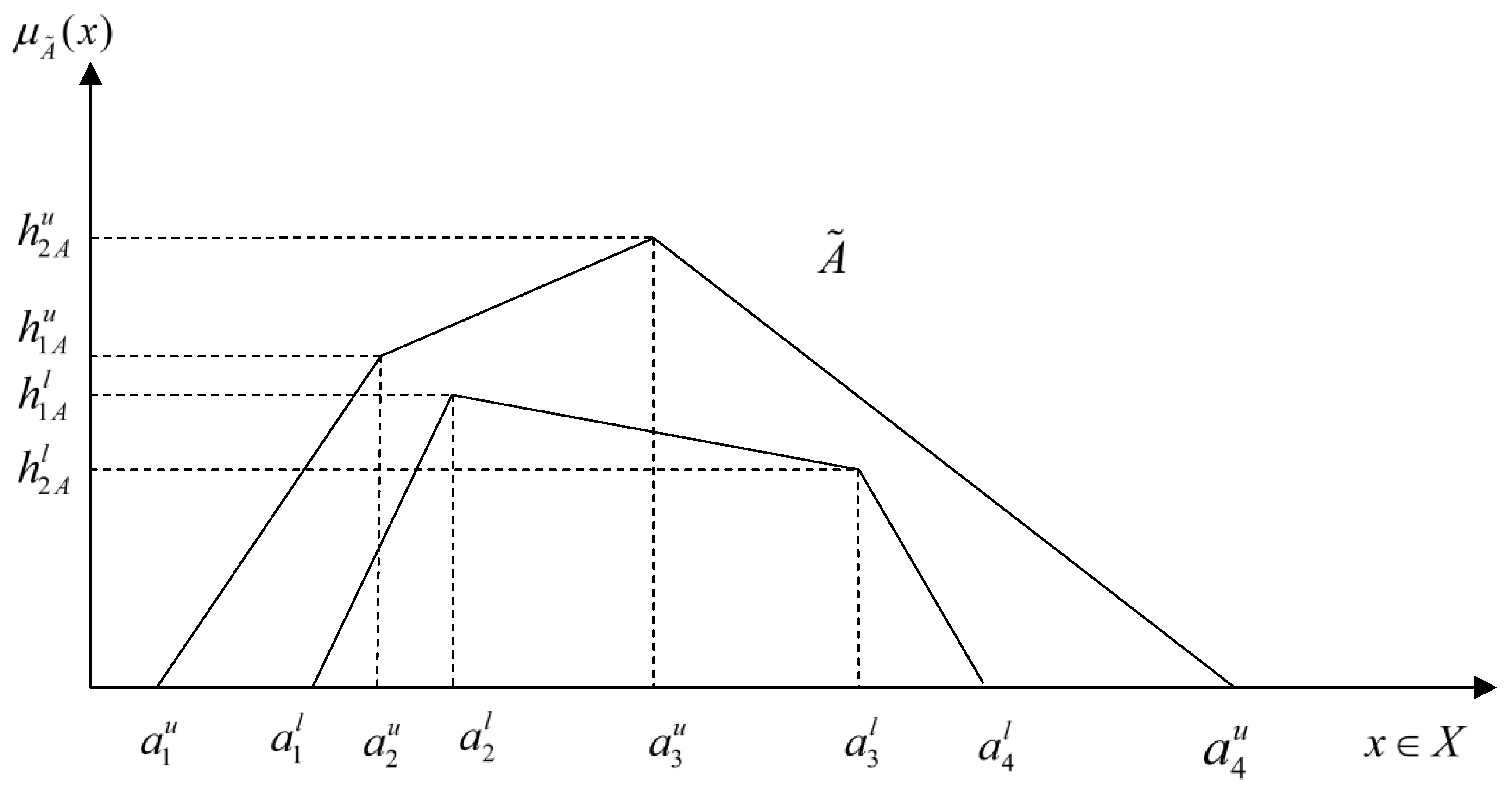
2.3. T2 Fuzzy Set and Its Order Relations
2.4. Pseudo-Interval T2 Fuzzy Sets Linear Program
2.5. Bi-Objective Pseudo-Interval T2 Linear Program
3. Case Study
3.1. Overview
3.2. Model Framework
4. Results and Discussion
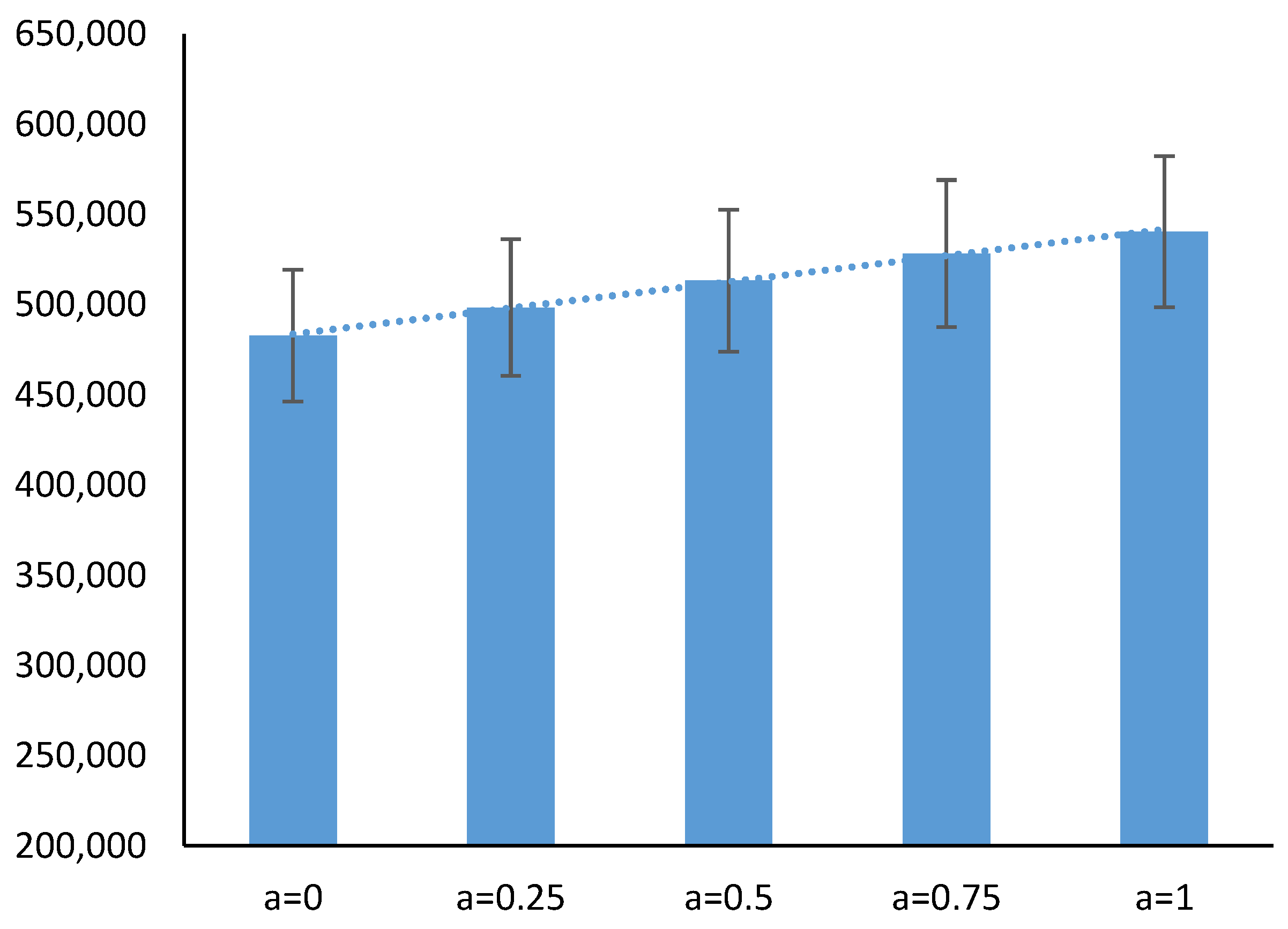
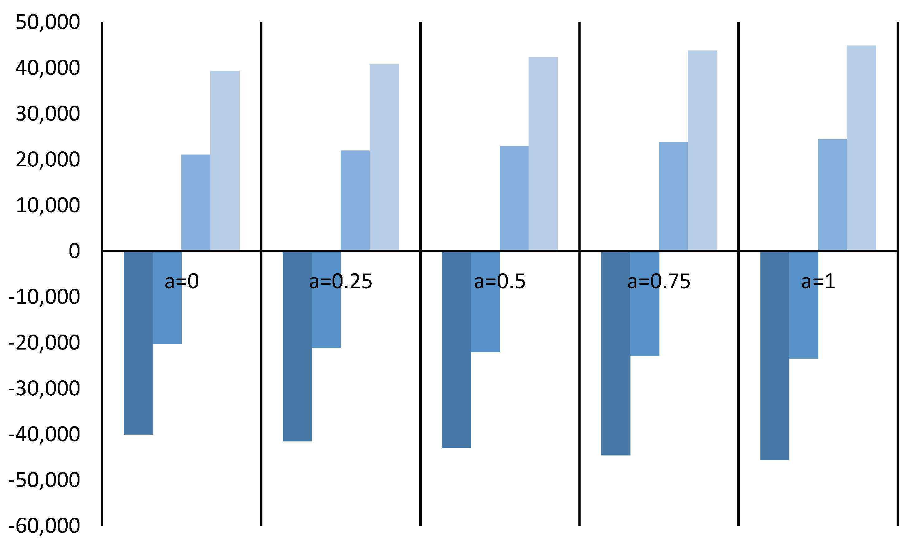
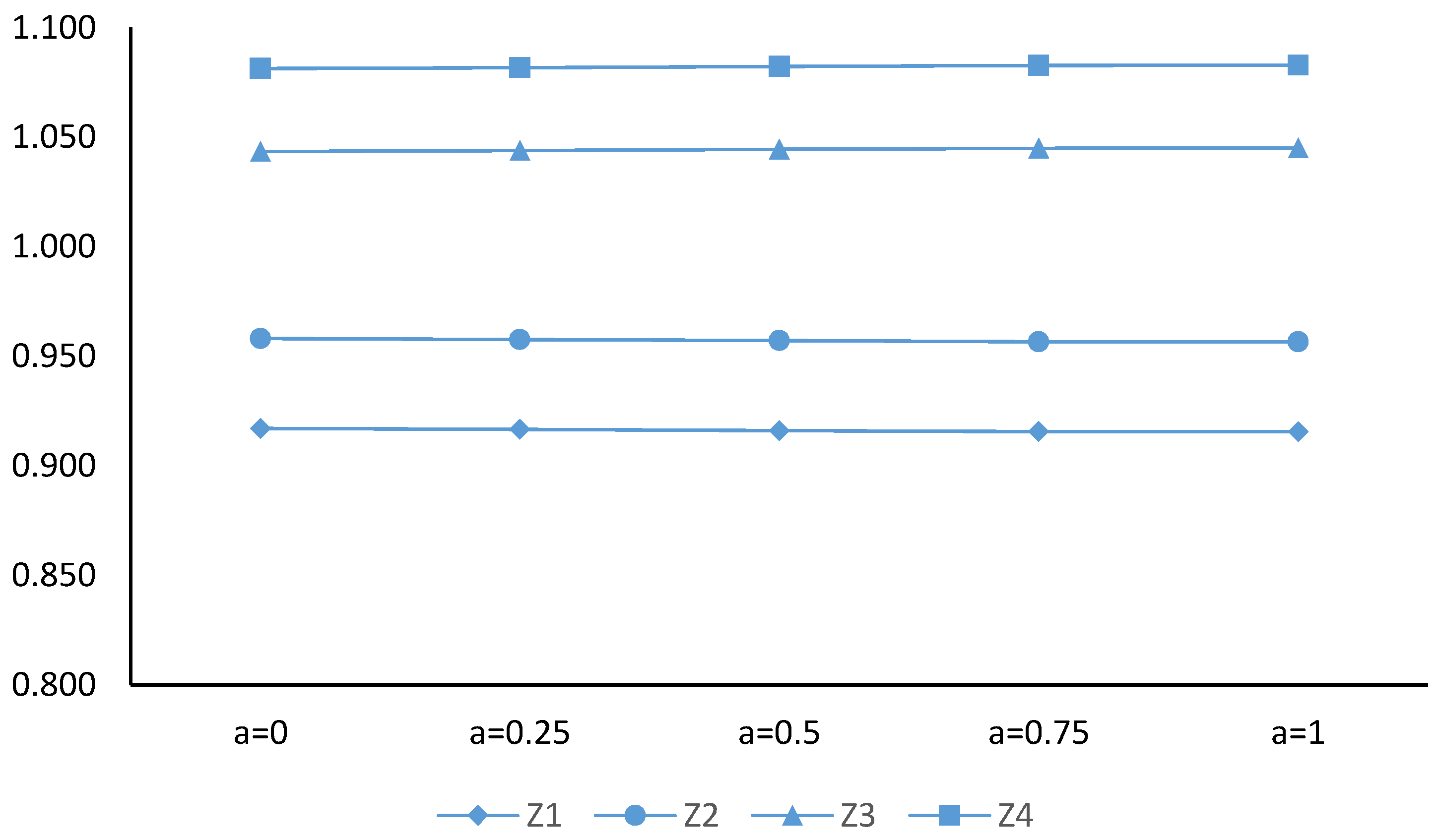
4.1. Bi-Objective Water Model Solutions
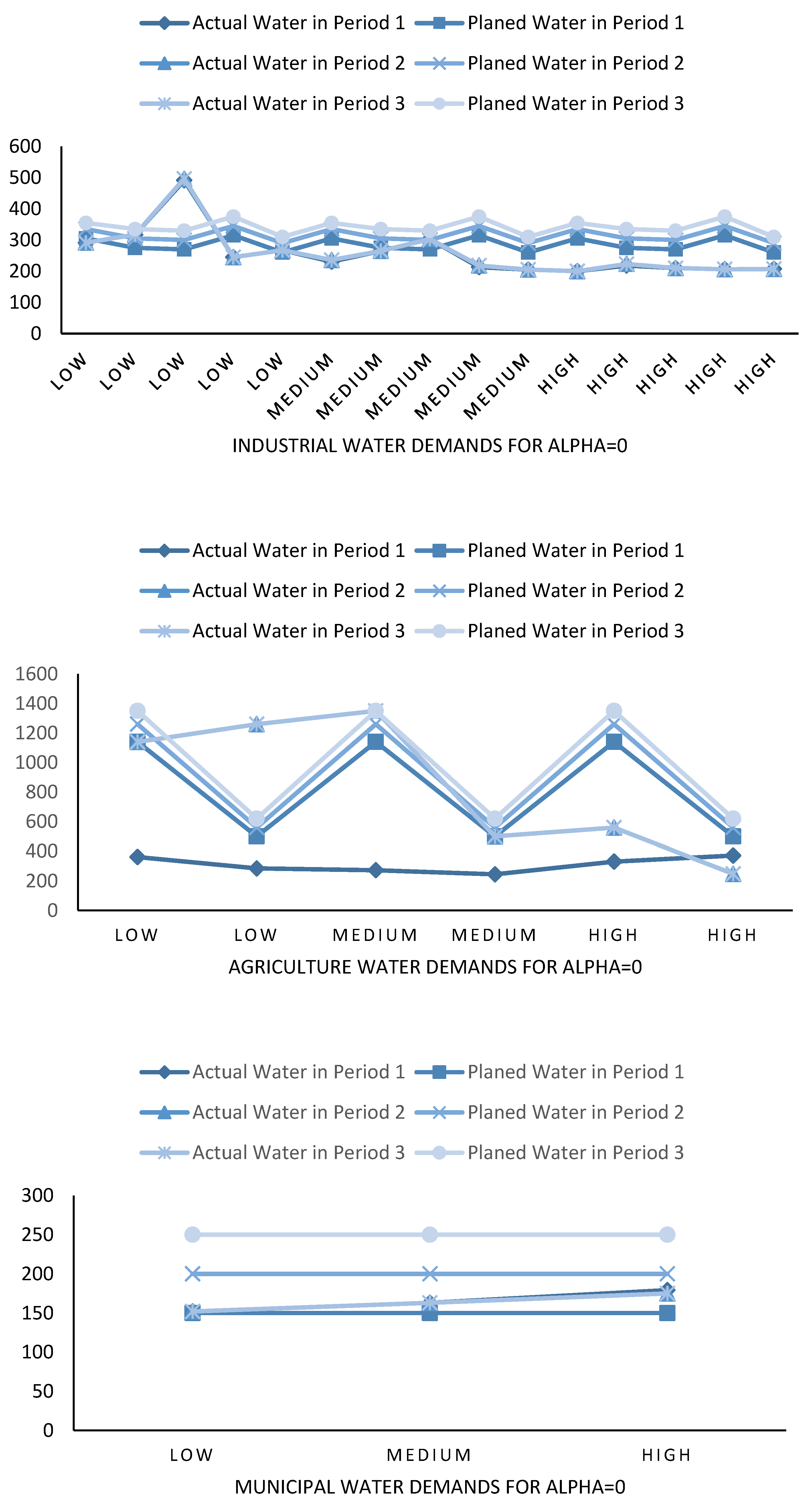
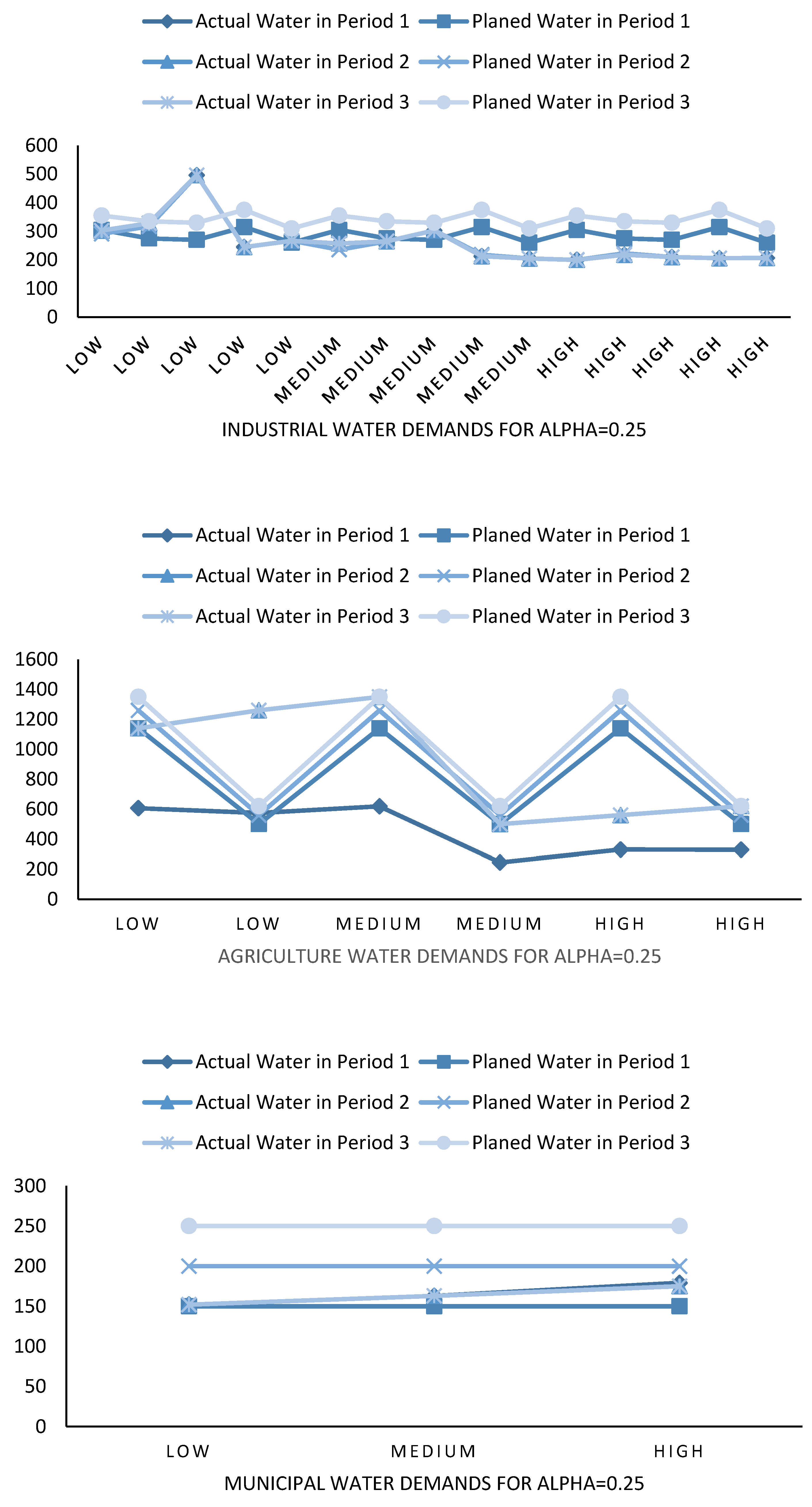
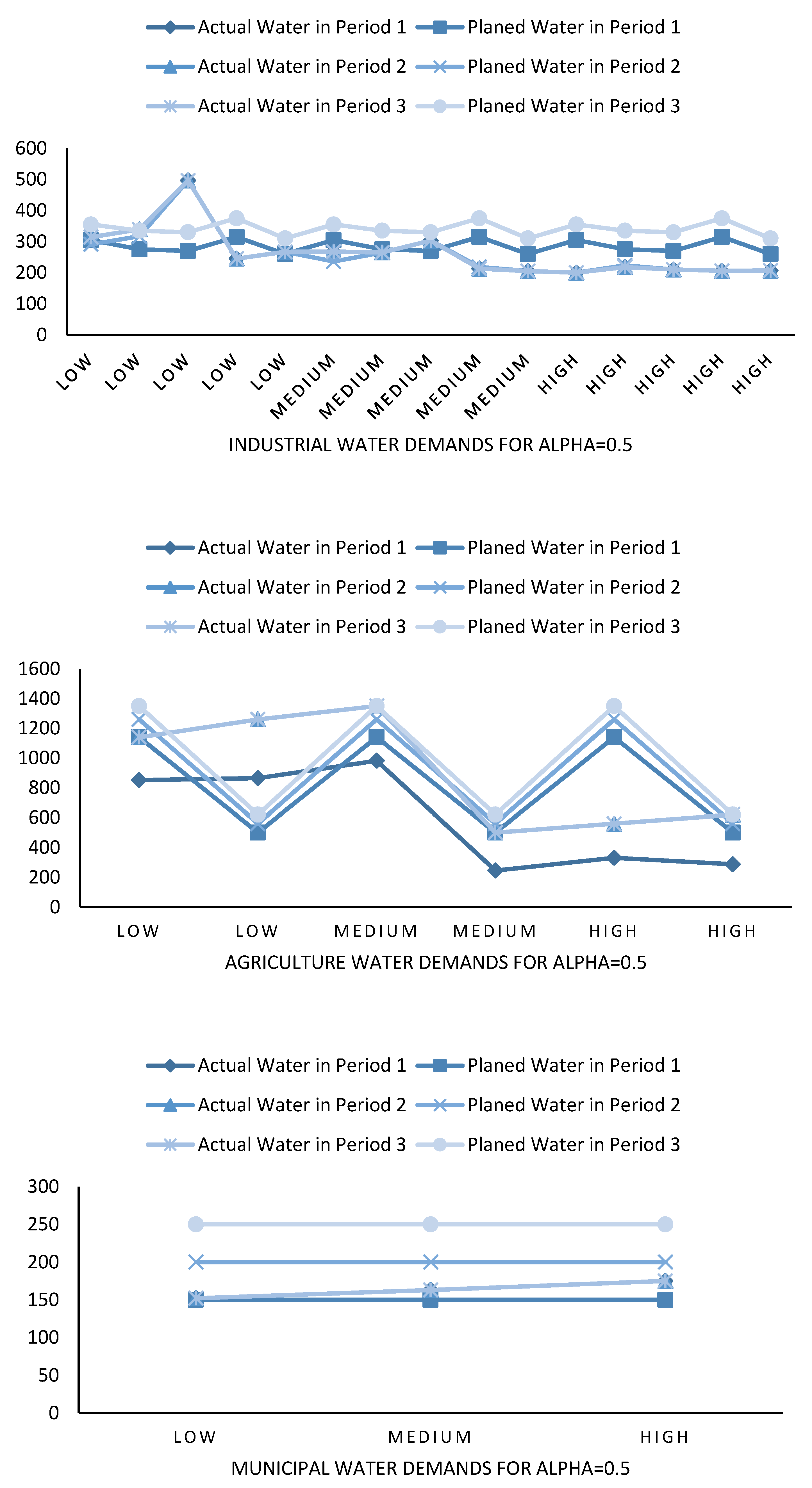
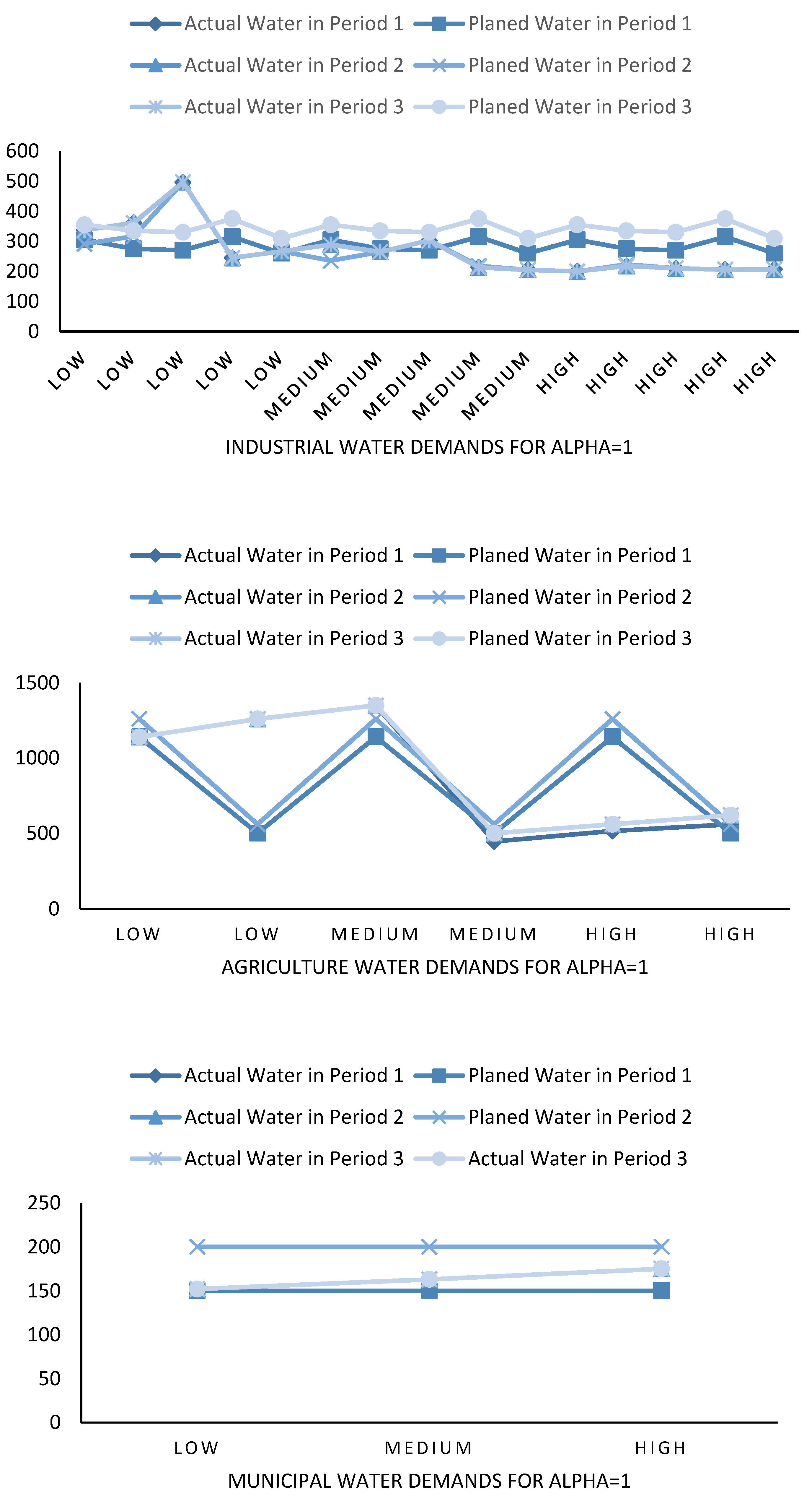
4.2. Water Demands of End-Users
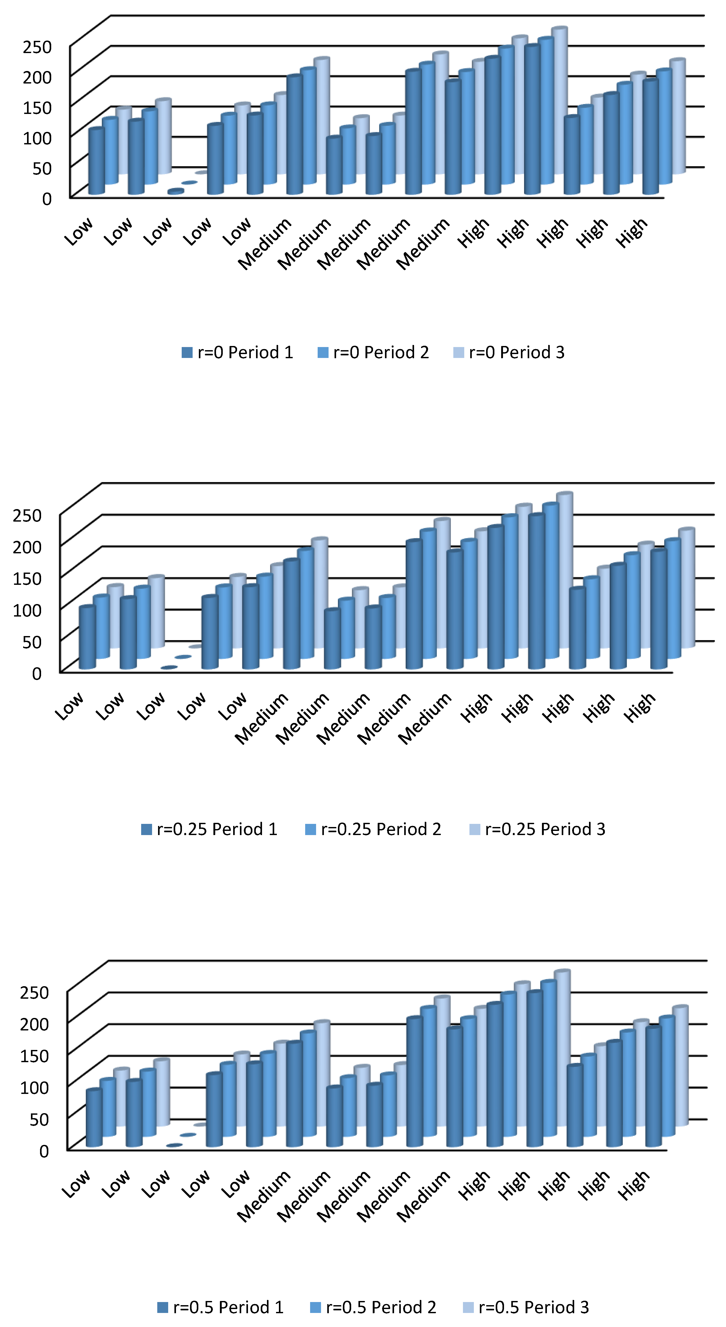
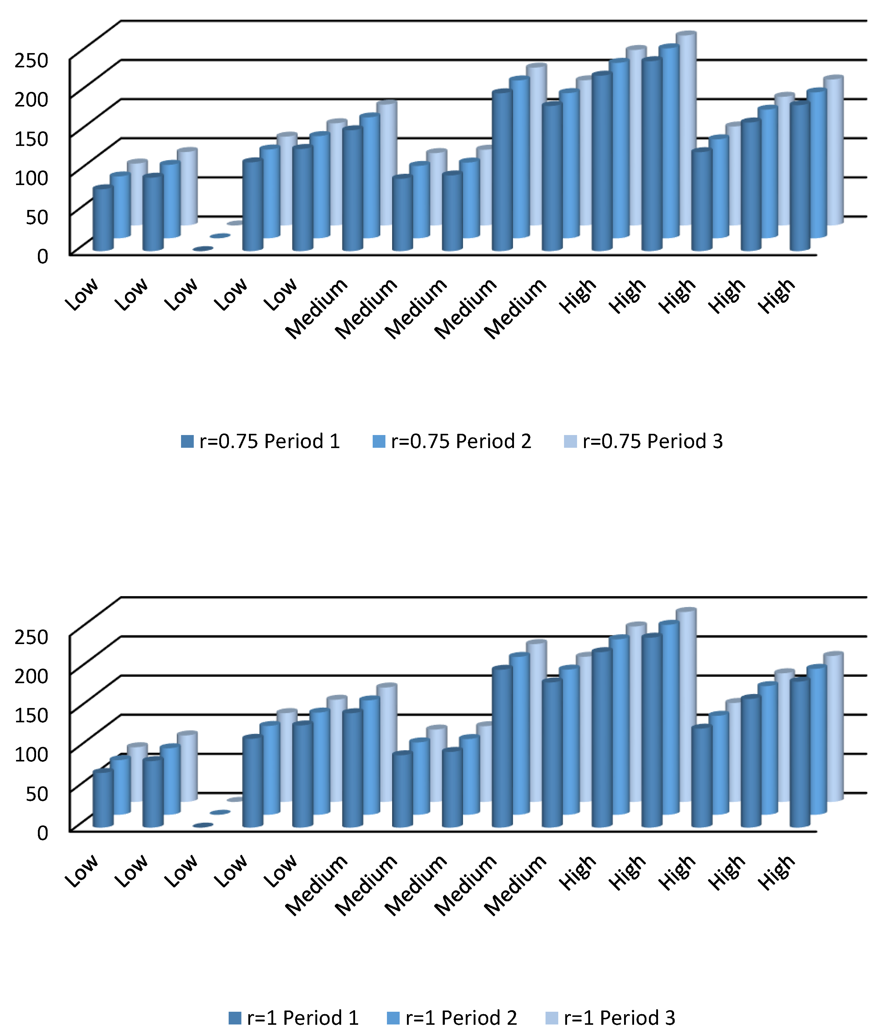
4.3. Recycled Water Demands
4.4. Comparative Analysis
5. Conclusions
Author Contributions
Acknowledgments
Conflicts of Interest
Abbreviations
| Notation | |
| i | five subcategories of industrial classification, namely, petrochemical industry, information technology industry, machinery industry, biotechnology industry, and marine technology industry; |
| a | two categories of agricultural classification, namely, crop agriculture and animal husbandry; |
| t | three five-year plans of China; |
| h | water inflow level (h = 1, 2, and 3 for low, medium, and high level, respectively); |
| industrial raw water volume, m3; | |
| industrial reuse water volume, m3; | |
| industrial unit water profit, yuan/m3; | |
| agricultural raw water volume, m3; | |
| agricultural unit water profit, yuan/m3; | |
| municipal water consumption, m3; | |
| municipal reuse water volume, m3; | |
| municipal unit water profit, yuan/m3; | |
| water shortage for the industrial categories, m3; | |
| unit reduction in the net benefit when the water supply target is not delivered to the industrial categories, yuan/m3; | |
| water shortage for the agricultural categories, m3; | |
| reduction in the net benefit when the water supply target is not delivered to the agricultural categories, yuan/m3; | |
| water shortage for the municipal bodies, m3; | |
| reduction in the net benefit when the water supply target is not delivered to the municipal bodies, yuan/m3; | |
| industrial reuse water unit water supply cost, yuan/m3; | |
| municipal reuse water cost, yuan/m3; | |
| industrial sewage treatment cost, yuan/m3; | |
| industrial sewage production rate; | |
| municipal sewage treatment cost, yuan/m3; | |
| municipal sewage production rate; | |
| municipal water consumption, m3; | |
| total water available in the area, 104 m3; | |
| amount of water demand for the industrial categories, m3; | |
| amount of water demand for the agricultural categories, m3; | |
| amount of water demand for the municipal bodies, m3; | |
| reduced rainfall, 108 m3; | |
| industrial wastewater discharge rate; | |
| municipal wastewater discharge rate; | |
| capacity of the sewage treatment, m3 |
References
- Huang, Y.; Chen, X.; Li, Y.; Willems, P.; Liu, T. Integrated modeling system for water resources management of Tarim River Basin. Environ. Eng. Sci. 2010, 27, 255–269. [Google Scholar] [CrossRef]
- Jin, L.; Huang, G.; Fan, Y.; Nie, X.; Cheng, G. A hybrid dynamic dual interval programming for irrigation water allocation under uncertainty. Water Resour. Manag. 2012, 26, 1183–1200. [Google Scholar] [CrossRef]
- Li, Y.; Huang, G.; Nie, S. An interval-parameter multi-stage stochastic programming model for water resources management under uncertainty. Adv. Water Resour. 2006, 29, 776–789. [Google Scholar] [CrossRef]
- Li, Y.; Huang, G.H.; Huang, Y.; Zhou, H. A multistage fuzzy-stochastic programming model for supporting sustainable water-resources allocation and management. Environ. Model. Softw. 2009, 24, 786–797. [Google Scholar] [CrossRef]
- Luo, B.; Maqsood, I.; Yin, Y.; Huang, G.; Cohen, S. Adaption to climate change through water trading under uncertainty-An inexact two-stage nonlinear programming approach. J. Environ. Inf. 2015, 2, 58–68. [Google Scholar] [CrossRef]
- Nematian, J. An extended two-stage stochastic programming approach for water resources management under uncertainty. J. Environ. Inform. 2016, 27. [Google Scholar] [CrossRef]
- Thissen, W.; Kwakkel, J.; Mens, M.; Van der Sluijs, J.; Stemberger, S.; Wardekker, A.; Wildschut, D. Dealing with uncertainties in fresh water supply: Experiences in the Netherlands. Water Resour. Manag. 2017, 31, 703–725. [Google Scholar] [CrossRef]
- Liu, D.; Liu, W.; Fu, Q.; Zhang, Y.; Li, T.; Imran, K.M.; Abrar, F.M. Two-stage multi-water sources allocation model in regional water resources management under uncertainty. Water Resour. Manag. 2017, 31, 3607–3625. [Google Scholar] [CrossRef]
- Parker, G.G.; Ferguson, G.E.; Love, S.K. Water Resources of Southeastern Florida, with Special Reference to Geology and Ground Water of the Miami Area; U.S. G.P.O.: Washington, WA, USA, 1955.
- Abdulbaki, D.; Al-Hindi, M.; Yassine, A.; Najm, M.A. An optimization model for the allocation of water resources. J. Clean. Prod. 2017, 164, 994–1006. [Google Scholar] [CrossRef]
- Celik, E.; Gul, M.; Aydin, N.; Gumus, A.T.; Guneri, A.F. A comprehensive review of multi criteria decision making approaches based on interval type-2 fuzzy sets. Knowl.-Based Syst. 2015, 85, 329–341. [Google Scholar] [CrossRef]
- Ahmad, A.; El-Shafie, A.; Razali, S.F.M.; Mohamad, Z.S. Reservoir optimization in water resources: A review. Water Resour. Manag. 2014, 28, 3391–3405. [Google Scholar] [CrossRef]
- Daghighi, A.; Nahvi, A.; Kim, U. Optimal cultivation pattern to increase revenue and reduce water use: Application of linear programming to arjan plain in Fars province. Agriculture 2017, 7, 73. [Google Scholar] [CrossRef]
- Miao, D.; Huang, W.; Li, Y.; Yang, Z. Planning water resources systems under uncertainty using an interval-fuzzy de novo programming method. J. Environ. Inform. 2014, 24. [Google Scholar] [CrossRef]
- Wang, S.; Huang, G. A multi-level Taguchi-factorial two-stage stochastic programming approach for characterization of parameter uncertainties and their interactions: An application to water resources management. Eur. J. Oper. Res. 2015, 240, 572–581. [Google Scholar] [CrossRef]
- Chen, Y.; He, L.; Lu, H.; Li, J.; Ren, L. Planning for regional water system sustainability through water resources security assessment under uncertainties. Water Resour. Manag. 2018, 32, 3135–3153. [Google Scholar] [CrossRef]
- Dai, R.; Charkhgard, H. A two-stage approach for bi-objective integer linear programming. Oper. Res. Lett. 2018, 46, 81–87. [Google Scholar] [CrossRef]
- Charkhgard, H.; Eshragh, A. Best subset selection in linear regression via bi-objective mixed integer linear programming. arXiv, 2018; arXiv:1804.07935. [Google Scholar]
- Saghand, P.G.; Charkhgard, H.; Kwon, C. A branch-and-bound algorithm for a class of mixed integer linear maximum multiplicative programs: A bi-objective optimization approach. Comput. Oper. Res. 2018, 101, 263–274. [Google Scholar] [CrossRef]
- Naderi, M.; Pishvaee, M. Robust bi-objective macroscopic municipal water supply network redesign and rehabilitation. Water Resour. Manag. 2017, 31, 2689–2711. [Google Scholar] [CrossRef]
- Irawan, C.A.; Jones, D.; Ouelhadj, D. Bi-objective optimisation model for installation scheduling in offshore wind farms. Comput. Oper. Res. 2017, 78, 393–407. [Google Scholar] [CrossRef]
- Belmonte, B.A.; Benjamin, M.F.D.; Tan, R.R. Bi-objective optimization of biochar-based carbon management networks. J. Clean. Prod. 2018, 188, 911–920. [Google Scholar] [CrossRef]
- Vahdani, B.; Tavakkoli-Moghaddam, R.; Jolai, F.; Baboli, A. Reliable design of a closed loop supply chain network under uncertainty: An interval fuzzy possibilistic chance-constrained model. Eng. Optim. 2013, 45, 745–765. [Google Scholar] [CrossRef]
- Huang, G.H.; Baetz, B.W.; Patry, G.G. A grey fuzzy linear programming approach for municipal solid waste management planning under uncertainty. Civ. Eng. Syst. 1993, 10, 123–146. [Google Scholar] [CrossRef]
- Jin, L.; Huang, G.H.; Wang, L.; Wang, X. Robust fully fuzzy programming with fuzzy set ranking method for environmental systems planning under uncertainty. Environ. Eng. Sci. 2013, 30, 280–293. [Google Scholar] [CrossRef]
- Baky, I.A. Fuzzy goal programming algorithm for solving decentralized bi-level multi-objective programming problems. Fuzzy Sets Syst. 2009, 160, 2701–2713. [Google Scholar] [CrossRef]
- Sinha, S. Fuzzy programming approach to multi-level programming problems. Fuzzy Sets Syst. 2003, 136, 189–202. [Google Scholar] [CrossRef]
- Kumar, D.; Rahman, Z.; Chan, F.T. A fuzzy AHP and fuzzy multi-objective linear programming model for order allocation in a sustainable supply chain: A case study. Int. J. Comput. Integr. Manuf. 2017, 30, 535–551. [Google Scholar] [CrossRef]
- Takami, M.A.; Sheikh, R.; Sana, S.S. A hesitant fuzzy set theory based approach for project portfolio selection with interactions under uncertainty. J. Inf. Sci. Eng. 2018, 34, 65–79. [Google Scholar]
- Zadeh, L. Fuzzy sets. Inf. Control 1965, 8, 338–353. [Google Scholar] [CrossRef]
- Huang, G.H. IPWM: An interval parameter water quality management model. Eng. Optim. 1996, 26, 79–103. [Google Scholar] [CrossRef]
- Hu, C.; Kearfott, R.B.; De Korvin, A.; Kreinovich, V. Knowledge Processing with Interval and Soft Computing; Springer: London, UK, 2008; ISBN 978-1-84800-325-5. [Google Scholar]
- Dong, J.Y.; Wan, S.P. A new trapezoidal fuzzy linear programming method considering the acceptance degree of fuzzy constraints violated. Knowl.-Based Syst. 2018, 148, 100–114. [Google Scholar] [CrossRef]
- Ishibuchi, H.; Tanaka, H. Multiobjective programming in optimization of the interval objective function. Eur. J. Oper. Res. 1990, 48, 219–225. [Google Scholar] [CrossRef]
- Karnik, N.N.; Mendel, J.M. Operations on type-2 fuzzy sets. Fuzzy Sets Syst. 2001, 122, 327–348. [Google Scholar] [CrossRef]
- Srinivasan, A.; Geetharamani, G. Linear programming problem with interval type 2 fuzzy coefficients and an interpretation for ITS constraints. J. Appl. Math. 2016, 1, 1–11. [Google Scholar] [CrossRef]
- Jin, L.; Huang, G.; Cong, D.; Fan, Y. A robust inexact joint-optimal α cut interval type-2 fuzzy boundary linear programming (RIJ-IT2FBLP) for energy systems planning under uncertainty. Int. J. Electr. Power Energy Syst. 2014, 56, 19–32. [Google Scholar] [CrossRef]
- Statistical Communique of Xiamen’s City Economic and Social Development Xiamen Statistics Bureau. Available online: http://www.stats-xm.gov.cn/ (accessed on 28 May 2018).
- Kuriqi, A. Simulink application on dynamic modelling of biological wastewater treatment for aerator tank case. Int. J. Sci. Technol. Res. 2014, 3, 69–72. [Google Scholar]
- Kuriqi, A.; Kuriqi, I.; Poci, E. Simulink Programming for Dynamic Modelling of Activated Sludge Process: Aerator and Settler Tank Case. Fresen. Environ. Bull. 2016, 25, 2891. [Google Scholar]
- Zhao, J.; Li, M.; Guo, P.; Zhang, C.; Tan, Q. Agricultural water productivity-oriented water resources allocation based on the coordination of multiple factors. Water 2017, 9, 490. [Google Scholar] [CrossRef]


| Periods | |||
|---|---|---|---|
| t = 1 | t = 2 | t = 3 | |
| Industrial Users | |||
| i = 1 | 305 | 335 | 355 |
| i = 2 | 275 | 305 | 335 |
| i = 3 | 270 | 300 | 330 |
| i = 4 | 315 | 345 | 375 |
| i = 5 | 260 | 290 | 310 |
| Agriculture Users | |||
| a = 1 | 1140 | 1180 | 1210 |
| a = 2 | 500 | 560 | 586 |
| Municipal Users | |||
| m = 1 | [53.2, 54.6] | [54.2, 55.6] | [55.2, 56.6] |
| Probability | Periods | |||
|---|---|---|---|---|
| t = 1 | t = 2 | t = 3 | ||
| Total available water resources (106) | ||||
| Low | 0.25 | (738, 820, 1228, 1345) | (758, 820, 1248, 1365) | (778, 840, 1268, 1385) |
| Medium | 0.5 | (1350, 1420, 2170, 2250) | (1370, 1440, 2190, 2270) | (1390, 1460, 2210, 2290) |
| High | 0.25 | (2260, 2350, 3560, 3650) | (2280, 2370, 3580, 3670) | (2300, 2390, 3600, 3690) |
| Water demand | ||||
| Industrial users | ||||
| i = 1 | (520, 580, 681, 702) | (540, 600, 701, 722) | (560, 620, 721, 742) | |
| i = 2 | (610, 631, 712, 750) | (620, 651, 732, 770) | (640, 671, 752, 790) | |
| i = 3 | (620, 650, 730, 762) | (640, 670, 750, 782) | (660, 690, 770, 802) | |
| i = 4 | (530, 552, 660, 689) | (550, 572, 680, 709) | (570, 592, 700, 729) | |
| i = 5 | (552, 580, 678, 708) | (572, 600, 698, 728) | (592, 620, 718, 748) | |
| Agricultural users | ||||
| a = 1 | (1110, 1142, 1201, 1215) | (1150, 1162, 1241, 1265) | (1200, 1262, 1341, 1365) | |
| a = 2 | (510, 542, 601, 615) | (550, 582, 651, 685) | (580, 602, 705, 752) | |
| Municipal users | (52, 60, 72, 80) | (60, 68, 78, 85) | (65, 72, 85, 90) | |
| Net Benefit for Water Utilization | Penalty Cost for Water Shortage | |||||
|---|---|---|---|---|---|---|
| T = 1 | T = 2 | T = 3 | T = 1 | T = 2 | T = 3 | |
| Industry Users | ||||||
| i = 1 | (190, 193, 201, 203) | (190, 195, 200, 203) | (199, 201, 204, 206) | (210, 213, 221, 223) | (210, 215, 220, 223) | (219, 221, 224, 226) |
| i = 2 | (138, 141, 146, 149) | (138, 140, 146, 148) | (144, 142, 148, 150) | (158, 161, 166, 169) | (158, 160, 166, 168) | (164, 162, 168, 170) |
| i = 3 | (132, 135, 139, 142) | (133, 135, 142, 145) | (133, 135, 142, 145) | (152, 155, 159, 162) | (153, 155, 162, 165) | (153, 155, 162, 165) |
| i = 4 | (123, 125, 130, 133) | (124, 126, 130, 134) | (127, 129, 133, 136) | (143, 145, 150, 153) | (144, 146, 150, 154) | (147, 149, 153, 156) |
| i = 5 | (108, 110, 115, 118) | (110, 113, 118, 120) | (110, 112, 118, 120) | (128, 130, 135, 138) | (130, 133, 138, 140) | (130, 132, 138, 140) |
| Agriculture Users | ||||||
| a = 1 | (28, 30, 38, 40) | (33, 35, 42, 45) | (35, 38, 46, 48) | (38, 40, 48, 50) | (43, 45, 52, 55) | (45, 48, 56, 58) |
| a = 2 | (90, 92, 94, 96) | (92, 95, 98, 100) | (90, 93, 96, 98) | (100, 102, 104, 106) | (102, 105, 108, 110) | (100, 103, 106, 108) |
| Municipal Users | ||||||
| m = 1 | (4.8, 5.0, 5.8, 6.0) | (5.0, 5.2, 6.0, 6.2) | (5.5, 5.8, 6.5, 6.8) | (5.8, 6.0, 6.8, 7.0) | (6.0, 6.2, 6.5, 7.0) | (6.5, 6.8, 7.0, 7.2) |
| Acceptance Degree α | Z = 1 | Z = 2 | Z = 3 | Z = 4 |
|---|---|---|---|---|
| α = 0.00 | 442,784.0 | 462,602.6 | 503,821.3 | 522,116.7 |
| α = 0.25 | 456,804.5 | 477,254.1 | 520,284.2 | 539,127.9 |
| α = 0.50 | 470,247.9 | 491,303.5 | 536,161.5 | 555,563.4 |
| α = 0.75 | 483,695.5 | 505,357.3 | 552,043.6 | 572,003.8 |
| α = 1.00 | 494,742.1 | 516,920.9 | 564,739.2 | 585,211.6 |
| Periods | ||||
|---|---|---|---|---|
| Water Levels | t = 1 | t = 2 | t = 3 | |
| Industrial Consumers | ||||
| i = 1 | Low | 291.2, 302.5, 314.1, 325.5, 337 | 291.2, 302.5, 314.1, 325.5, 337 | 291.2, 302.5, 314.1, 325.5, 337 |
| i = 2 | Low | 317.1, 328.2, 339.3, 350.4, 361.5 | 317.1, 328.2, 339.3, 350.4, 361.5 | 317.1, 328.2, 339.3, 350.4, 361.5 |
| i = 3 | Low | 491.2, 496.3, 496.3, 496.3, 496.3 | 496.3 | 496.3 |
| i = 4 | Low | 245 | 245 | 245 |
| i = 5 | Low | 267 | 267 | 267 |
| i = 1 | Medium | 230.6, 257.4, 267.8, 278.2, 288.7 | 235.7, 257.4, 267.8, 278.2, 288.7 | 235.7, 257.4, 267.8, 278.2, 288.7 |
| i = 2 | Medium | 265 | 265 | 265 |
| i = 3 | Medium | 303 | 303 | 303 |
| i = 4 | Medium | 213 | 218.1, 213, 213, 213, 213 | 218.1, 213, 213, 213, 213 |
| i = 5 | Medium | 205 | 205 | 205 |
| i = 1 | High | 200 | 200 | 200 |
| i = 2 | High | 218 | 223.1, 218, 218, 218, 218 | 223.1, 218, 218, 218, 218 |
| i = 3 | High | 210 | 210 | 210 |
| i = 4 | High | 206 | 206 | 206 |
| i = 5 | High | 207 | 207 | 207 |
| Agriculture Users | ||||
| a = 1 | Low | 362.1, 606.7, 851.3, 1095.8, 1140 | 1140 | 1140 |
| a = 2 | Low | 285.1, 575, 864.9, 1154.7, 1260 | 1260 | 1260 |
| a = 1 | Medium | 273, 618.9, 981.9, 1344.8, 1350 | 1350 | 1350 |
| a = 2 | Medium | 245, 245, 245, 245, 445.4 | 500 | 500 |
| a = 1 | High | 331, 331, 331, 331, 515.6 | 560 | 560 |
| a = 2 | High | 372, 329.5, 287, 244.5, 559.7 | 248, 620, 620, 620, 620 | 248, 620, 620, 620, 620 |
| Municipal Users | ||||
| m = 1 | Low | 152 | 152 | 152 |
| m = 1 | Medium | 163 | 163 | 163 |
| m = 1 | High | 175 | 175 | 175 |
| Periods | ||||
|---|---|---|---|---|
| Water Levels | t = 1 | t = 2 | t = 3 | |
| Industrial Consumers | ||||
| i = 1 | Low | 88.1 | 88.1 | 88.1 |
| i = 2 | Low | 102.7 | 102.7 | 102.7 |
| i = 3 | Low | 0 | 0 | 0 |
| i = 4 | Low | 113.4 | 113.4 | 113.4 |
| i = 5 | Low | 130.5 | 130.5 | 130.5 |
| i = 1 | Medium | 162.8 | 162.8 | 162.8 |
| i = 2 | Medium | 92.4 | 92.4 | 92.4 |
| i = 3 | Medium | 96.7 | 96.7 | 96.7 |
| i = 4 | Medium | 201.6 | 201.6 | 201.6 |
| i = 5 | Medium | 185.4 | 185.4 | 185.4 |
| i = 1 | High | 224.1 | 224.1 | 224.1 |
| i = 2 | High | 242.6 | 242.6 | 242.6 |
| i = 3 | High | 126.4 | 126.4 | 126.4 |
| i = 4 | High | 164.3 | 164.3 | 164.3 |
| i = 5 | High | 186.4 | 186.4 | 186.4 |
| Agriculture Users | ||||
| a = 1 | Low | 288.8 | 0 | 0 |
| a = 2 | Low | 395.1 | 0 | 0 |
| a = 1 | Medium | 368.2 | 0 | 0 |
| a = 2 | Medium | 255 | 0 | 0 |
| a = 1 | High | 229 | 0 | 0 |
| a = 2 | High | 333 | 0 | 0 |
| Municipal Users | ||||
| m = 1 | Low | 0 | 0 | 0 |
| m = 1 | Medium | 37 | 37 | 37 |
| m = 1 | High | 75 | 75 | 75 |
| Industrial Category | a = 0.0 | a = 0.25 | a = 0.50 | a = 0.75 | a = 1.0 |
|---|---|---|---|---|---|
| Petrochem 1 | 92.63 | 94.92167 | 97.21333 | 99.505 | 101.7967 |
| Petrochem 2 | 102.5452 | 104.7629 | 106.9806 | 109.1984 | 111.4161 |
| Petrochem 3 | 141.25 | 141.25 | 141.25 | 141.25 | 141.25 |
| Infotech 1 | 83.4 | 83.4 | 83.4 | 83.4 | 83.4 |
| Infotech 2 | 92.52 | 92.52 | 92.52 | 92.52 | 92.52 |
| Infotech 3 | 89.14156 | 93.47917 | 95.5625 | 97.64583 | 99.72917 |
| Machinery 1 | 87.4 | 87.4 | 87.4 | 87.4 | 87.4 |
| Machinery 2 | 99.72 | 99.72 | 99.72 | 99.72 | 99.72 |
| Machinery 3 | 85.61697 | 84.6 | 84.6 | 84.6 | 84.6 |
| Biotech 1 | 75.4 | 75.4 | 75.4 | 75.4 | 75.4 |
| Biotech 2 | 79.12 | 79.12 | 79.12 | 79.12 | 79.12 |
| Biotech 3 | 86.61697 | 85.6 | 85.6 | 85.6 | 85.6 |
| Marine tech 1 | 76.4 | 76.4 | 76.4 | 76.4 | 76.4 |
| Marine tech 2 | 80.32 | 80.32 | 80.32 | 80.32 | 80.32 |
| Marine tech 3 | 83.4 | 83.4 | 83.4 | 83.4 | 83.4 |
© 2018 by the authors. Licensee MDPI, Basel, Switzerland. This article is an open access article distributed under the terms and conditions of the Creative Commons Attribution (CC BY) license (http://creativecommons.org/licenses/by/4.0/).
Share and Cite
Jin, L.; Fu, H.; Kim, Y.; Long, J.; Huang, G. A Bi-Objective Pseudo-Interval T2 Linear Programming Approach and Its Application to Water Resources Management Under Uncertainty. Water 2018, 10, 1545. https://doi.org/10.3390/w10111545
Jin L, Fu H, Kim Y, Long J, Huang G. A Bi-Objective Pseudo-Interval T2 Linear Programming Approach and Its Application to Water Resources Management Under Uncertainty. Water. 2018; 10(11):1545. https://doi.org/10.3390/w10111545
Chicago/Turabian StyleJin, Lei, Haiyan Fu, Younggy Kim, Jiangxue Long, and Guohe Huang. 2018. "A Bi-Objective Pseudo-Interval T2 Linear Programming Approach and Its Application to Water Resources Management Under Uncertainty" Water 10, no. 11: 1545. https://doi.org/10.3390/w10111545
APA StyleJin, L., Fu, H., Kim, Y., Long, J., & Huang, G. (2018). A Bi-Objective Pseudo-Interval T2 Linear Programming Approach and Its Application to Water Resources Management Under Uncertainty. Water, 10(11), 1545. https://doi.org/10.3390/w10111545