Shear-Thinning Fluid Flow in Variable-Aperture Channels

Abstract

Non-Newtonian fluid flow in a single fracture is a 3-D nonlinear phenomenon that is often averaged across the fracture aperture and described as 2-D. To capture the key interactions between fluid rheology and spatial heterogeneity, we adopt a simplified geometric model to describe the aperture variability, consisting of adjacent one-dimensional channels with constant aperture, each drawn from an assigned aperture distribution. The flow rate is then derived under the lubrication approximation for the two limiting cases of an external pressure gradient that is parallel/perpendicular to the channels; these two arrangements provide upper and lower bounds to the fracture conductance. The fluid rheology is described by the Prandtl–Eyring shear-thinning model. Novel closed-form results for the flow rate and hydraulic aperture are derived and discussed; different combinations of the parameters that describe the fluid rheology and the variability of the aperture field are considered. The flow rate values are very sensitive to the applied pressure gradient and to the shape of the distribution; in particular, more skewed distribution entails larger values of a dimensionless flow rate. Results for practical applications are compared with those valid for a power-law fluid and show the effects on the fracture flow rate of a shear stress plateau.

1. Introduction

Non-Newtonian fluid flow in fractured media is of interest for many environmentally related applications, such as hydraulic fracturing, drilling operations, enhanced oil recovery, and subsurface contamination and remediation. The basic building block in fractured media modeling is a thorough understanding of flow and transport in a single fracture [1]. A key concept in single-fracture flow and transport is the fracture aperture, defined by the space between the fracture walls. As a result of the heterogeneity of these surfaces, the fracture aperture is spatially variable. To model this variability, two basic approaches have been adopted. The first describes the aperture as a 2-D random field, typically described by an autocorrelation function of finite variance and integral scale [2]. The second envisages the aperture variability as the outcome of the joint variation in self-affine surfaces, correlated at all scales [3]. In both cases, flow modeling at the single-fracture scale leads to the determination of the flow rate under a given pressure gradient as a function of the parameters that describe the variability of the aperture field or of the confining walls. A hydraulic aperture can then be derived from the flow rate [4] as the aperture of a smooth-walled conduit that would produce the same flow rate under a given pressure gradient as the real rough-walled fracture.

When fluid behavior is non-Newtonian, the effects of spatial variability are compounded with the influence of rheology, producing striking results, such as pronounced channeling effects [5]. Different constitutive equations have been used to represent non-Newtonian behavior in fracture flow, ranging from the simpler two-parameter power-law model [5] to the four-parameter Carreau–Yasuda equation [6]. A comprehensive comparison of results for different constitutive equations is still lacking, but the impact of fluid rheology is likely to be significant in view of the diverse behavior of rheological equations in the vicinity of the zero-shear-rate limit [7].

Detailed 2-D or 3-D flow modeling of non-Newtonian flow in single fractures needs to be tackled numerically, with considerable computational effort, given the nonlinearity of the flow. Not surprisingly, some authors have pursued a simpler approach, with the aim of providing order of magnitude estimates and reference benchmarks for fracture conductivity. Basically, this approach considers a simplified, extremely anisotropic fracture geometry, with the aperture variable along one direction and constant-aperture channels along the other. The arbitrary orientation of the external pressure gradient with respect to the channels gives rise to two limit cases: (i) the parallel arrangement, which provides an upper bound to the conductivity, and (ii) the serial arrangement, which provides a lower bound. Flow in an isotropic aperture field is then addressed by considering the fracture as a random mixture of elements in which the fluid flows either transversal or parallel to the aperture variation. The hydraulic aperture is derived by a suitable averaging procedure, previously adopted for a deterministic aperture variation [8].

The present paper follows this avenue of research by exploring the impact of a classical, two-parameter shear-thinning constitutive equation, the Prandtl–Eyring model [9], which overcomes the unrealistic behavior of the power-law model, having infinite apparent viscosity for the zero shear rate.

Several suspensions of practical interest, such as magnetohydrodynamic (MHD) nanofluids, are well-interpreted by the Prandtl–Eyring model [10]. Many nanofluids are adopted in technologies such as fuel cells, microelectronics, and hybrid-powered engines. Nanofluids are used in industrial technologies because of their utility in the production of high-quality lubricants and oil, as they flow in fractures and small channels.

Section 2 derives the flow rate under an assigned external pressure gradient for the flow of a Prandtl–Eyring fluid in a parallel-plate fracture. Section 3 presents the simplified geometry adopted, derives general expressions of the flow rate for flow that is parallel or perpendicular to constant-aperture channels, and proposes a method to evaluate the hydraulic aperture for the 2-D case. Section 4 introduces a specific probability distribution function for the aperture—the gamma distribution—and illustrates results for the flow rate and hydraulic aperture for the two different 1-D cases. A dimensional comparison with results for the power-law fluid is drawn in Section 5. Conclusions and suggestions for future work are listed in Section 6.

2. Prandtl–Eyring Fluid Flow in Constant-Aperture Fracture

We consider the flow of a non-Newtonian Prandtl–Eyring fluid between two smooth parallel plates separated by a distance b (fracture aperture); the coordinate system is shown in Figure 1, with upper and lower plates at $z=\pm b/2$. A uniform pressure gradient $\overline{P_x}=-dP/dx$ is applied in the $x$-direction, where the generalized pressure $P=p+\rho gz$ includes gravity effects, $p$ is pressure, $g$ is gravity, and $\rho$ is fluid density. Assuming flow in the $x$-direction, the velocity $v_x$ is solely a function of $z$ under the hypothesis of infinite width W. Momentum balance yields a linear shear stress profile:

$${\tau }_{zx}=\overline{P_x} \left|z\right|$$

(1)

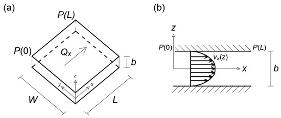
Figure 1. Parallel-plate model: (a) model representation and (b) cross-sectional velocity profile.

A Prandtl–Eyring fluid is described rheologically in simple shear flow by [9]:

$${\tau }_{zx}=A{\sinh }^{-1}\left(-\frac{1}{B}\frac{d{v}_x}{dz}\right),$$

(2)

where the parameter $B=1/\lambda$ of dimensions (T⁻¹) is the inverse of relaxation time $\lambda$, and the parameter $A$ is the Eyring characteristic shear tress of dimension (ML⁻¹T⁻²). For a vanishing shear rate ($d{v}_x/dz\equiv \dot{\gamma }\to 0$), the behavior tends to Newtonian with viscosity $\mu =A/B$, as is easily seen via the first-order expansion ${\sinh }^{-1}u\cong u.$ The behavior for a nonzero shear rate is shear-thinning, with a vanishing apparent viscosity for high shear stress. Figure 2 shows the apparent viscosity $\eta \left(\dot{\gamma }\right)$, defined by the relationship ${\tau }_{zx}=\eta \left(\dot{\gamma }\right)\dot{\gamma }$, as a function of the shear rate $\dot{\gamma }$, for realistic parameter values.

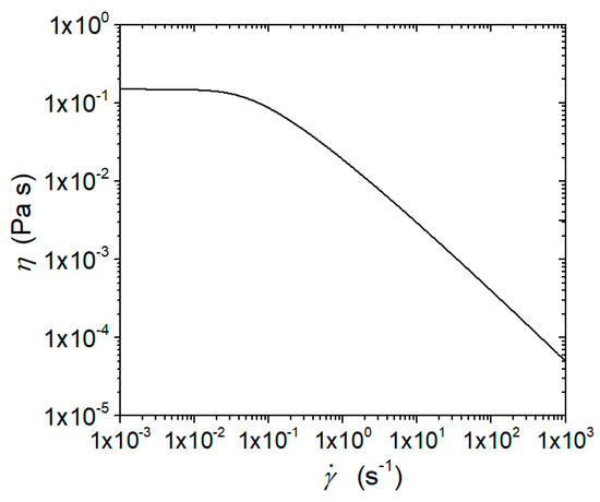
Figure 2. Prandtl–Eyring fluid rheology: apparent viscosity–shear rate relationship. Rheologic parameters from [7]: A = 0.00452 Pa and B = 0.0301 s⁻¹.

Substituting Equation (2) in Equation (1) and integrating with the no-slip condition at the wall $v_x\left(\mp b/2\right)=0$ gives the velocity profile between $z=-b/2$ and $z=+b/2$ as

$$v_x\left(z\right)=\frac{AB}{\overline{P_x}}\left[\cosh \left(\frac{\overline{P_x}b}{2A}\right)-\cosh \left(\frac{\overline{P_x}\left|z\right|}{A}\right)\right]$$

(3)

The total flow rate $Q_x$ through the fracture for a width $W$ in the y-direction perpendicular to the pressure gradient is derived by integrating Equation (2); the result is

$$Q_x=\frac{ABW}{\overline{P_x}}\left[b\cosh \left(\frac{\overline{P_x}b}{2A}\right)-\frac{2A}{\overline{P_x}}\sinh \left(\frac{\overline{P_x}b}{2A}\right)\right],$$

(4)

$$q_x=\frac{Q_x}{W},$$

(5)

$$V_x=\frac{q_x}{b},$$

(6)

where $q_x$ is the flow rate per unit width, and $V_x$ is the average velocity. For the vanishing dimensionless pressure gradient ($\overline{P_x}b/\left(2A\right)\to 0$), the hyperbolic functions can be replaced with their second-order expansions $\cosh u\cong 1+u^2/2$ and $\sinh u\cong u+u^3/6$, and the flow rate becomes

$$Q_x=\frac{1}{12}\frac{BW{b}^3}{A}\overline{P_x}=\frac{1}{12}\frac{W{b}^3}{{\mu }_0}\overline{P_x},$$

(7)

which is the “cubic law” [11] valid for a Newtonian fluid.

If the aperture varies, as in real rock fractures, a flow law of the type in Equations (4) and (5) is valid in replacing the constant aperture $b$ with a hydraulic (or flow or equivalent) aperture $b_H$, accounting for the variation in fracture aperture [8,12,13]. The availability of a closed-form expression for the hydraulic aperture as a function of fluid rheology and aperture variability is of particular interest in view of its use in numerical simulators.

3. Flow in Variable-Aperture Channels

Flow and transport simulations in variable-aperture fractures typically consider either the aperture $b\left(x,y\right)$ to vary as a two-dimensional, spatially homogeneous, and correlated random field with a probability density function $f\left(b\right)$ and assigned statistics, or to have walls described by a fractal distribution of a given Hurst coefficient H, correlated at all scales [3]. In the former case, the fracture dimensions are assumed to be much larger than the integral scale of the aperture autocovariance function; then, under ergodicity, spatial averages and ensemble averages are interchangeable, and a single realization can be examined [4]. This approach was followed by Di Federico [14] and Felisa et al. [15] to study the flow of power-law and truncated power-law fluids in simplified aperture fields in which the aperture varies only along one spatial coordinate, and the external pressure gradient (and hence the flow) is either transverse or parallel to the aperture variability; such an idealized fracture of dimensions $L$ and $W$ is shown in Figure 3. Here, we consider the flow of a Prandtl–Eyring fluid in both arrangements.

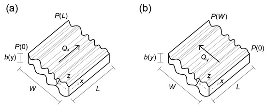
Figure 3. Conceptual model representation: (a) parallel arrangement and (b) serial arrangement.

3.1. Channels in Parallel

Consider flow along the direction $x$ parallel to constant-aperture channels and driven by the external pressure gradient $\overline{P_x}$, as illustrated in Figure 3a. To obtain the volumetric flux, a procedure similar to that adopted by Zimmerman and Bodvarsson [16] is used. The fracture, which has length $L$ and width $W$, is discretized into N neighboring parallel channels, which are all of equal width $W_i=W/N$, length $L$, and constant aperture $b_i$. Assuming that the shear between neighboring channels and the drag against the connecting walls may be neglected, the flow rate in each channel of a constant aperture along the $x$-direction is given by Equation (4) with $b_i$ in place of $b$ and $W_i$ in place of $W$. Hence, summing over all channels, the total flow rate in the fracture is

$$Q_x={\displaystyle \sum }_{i=1}^N{Q}_{xi}=\frac{ABW}{\overline{P_x}}\frac{1}{N}{\displaystyle \sum }_{i=1}^N\left[b_i\cosh \left(\frac{\overline{P_x}{b}_i}{2A}\right)-\frac{2A}{\overline{P_x}}\sinh \left(\frac{\overline{P_x}{b}_i}{2A}\right)\right].$$

(8)

Taking the limit as $N\to \infty$, the width of each channel tends to zero, and the discrete aperture variation tends to a continuous one; then, under ergodicity, Equation (8) gives the following expression for the flow rate per unit width:

$$q_x=\frac{Q_x}{W}=\frac{AB}{\overline{P_x}}\left[\underset{0}{\overset{\infty }{{\displaystyle \int }}}b\cosh \left(\frac{\overline{P_x}b}{2A}\right)f\left(b\right) \mathrm{d}b-\frac{2A}{\overline{P_x}}\underset{0}{\overset{\infty }{{\displaystyle \int }}}\sinh \left(\frac{\overline{P_x}b}{2A}\right)f\left(b\right) \mathrm{d}b\right],$$

(9)

where $f\left(b\right)$ is the probability distribution function of the aperture field $b$, defined between $0$ and $\infty$. Finally, the hydraulic aperture $b_{Hx}$ may be derived numerically by equating $q_x$ from Equation (9) to Equations (4) and (5) written with $b_{Hx}$ in place of $b$.

The assumption of negligible shear between neighboring channels in the limit $N\to \infty$ is equivalent to

$$\left|\frac{\partial {\tau }_{yx}}{\partial y}\right|\ll \left|\overline{P_x}\right|.$$

(10)

As a first approximation, the shear rate in the x–y plane due to a varying b is

$$\frac{\partial v_x}{\partial y}=\frac{B}{2}\sinh \left(\frac{\overline{P_x}b}{2A}\right)\frac{\partial b}{\partial y},$$

(11)

with a shear stress (see Equation (2)) equal to

$${\tau }_{yx}=-A{\sinh }^{-1}{\left[\frac{1}{2}\sinh \left(\frac{\overline{P_x}b}{2A}\right)\frac{\partial b}{\partial y}\right]}_{.}$$

(12)

Substituting into Equation (10) yields

$$\left|\cos \mathrm{h}\left(\frac{\left|\overline{P_x}\right|b}{2A}\right){\left(\frac{\partial b}{\partial y}\right)}^2+\frac{2A}{\left|\overline{P_x}\right|}\sin \mathrm{h}\left(\frac{\left|\overline{P_x}\right|b}{2A}\right)\frac{{\partial }^{2}b}{\partial y^2}\right|\ll 2\sqrt{4+{\left[\sin \mathrm{h}\left(\frac{\left|\overline{P_x}\right|b}{2A}\right)\right]}^2{\left(\frac{\partial b}{\partial y}\right)}^2}.$$

(13)

For smooth variation in b, with $\frac{\partial b}{\partial y}\to 0$ and $\frac{{\partial }^{2}b}{\partial y^2}\to 0$, the condition in Equation (13) is satisfied since, on the right-hand side, we have a finite-order term that is always >4, and on the left-hand side, we have a small-order term.

3.2. Channels in Series

Consider flow along the direction $y$ that is perpendicular to constant-aperture channels and driven by the external pressure gradient $\overline{P_y}$, case (b). The fracture, which has length $W$ and width $L$, is discretized into N cells in series of equal length $W_i=W/N$, each of width $L$ and constant aperture $b_i$. As volumetric flux $Q_y$ through each cell is the same, the flow rate per unit width in each cell is also the same, i.e., $q_{yi}=q_y=Q_y/L$. The total pressure loss along the fracture in the $y$-direction, $\Delta P$, can be expressed as the sum of pressure losses in each cell, $\Delta P_i$, as

$$\Delta P={\displaystyle \sum }_{i=1}^N\Delta P_i,$$

(14)

having neglected the pressure losses due to the succession of constrictions and enlargements. In turn, dividing by $W$ yields the external mean pressure gradient $\overline{P_y}$ as

$$\overline{P_y}=\frac{1}{N}{\displaystyle \sum }_{i=1}^N{P}_{yi},$$

(15)

where the pressure gradient in each cell of constant aperture $b_i$ is given by $P_{yi}=P_{yi}\left(q_y,b_i,A,B\right)$, which is obtained by deriving the pressure gradient as a function of flow rate from Equations (4) and (5), written by replacing the subscript $x$ with $y$ and $b$ with $b_i.$ Taking the limit as $N\to \infty$, the length of each cell tends to zero, and the discrete aperture variation tends to a continuous one; then, under ergodicity, Equation (15) gives the following expression for the mean pressure gradient in the $y$-direction:

$$\overline{P_y}=\underset{0}{\overset{\infty }{{\displaystyle \int }}}{P}_y\left(q_y,b,A,B\right)f\left(b\right)db.$$

(16)

The integration of Equation (16) implicitly gives the flow rate as $q_y=q_y\left(\overline{P_y},A,B, f\left(b\right)\right)$. Finally, the hydraulic aperture $b_{Hy}$ may be derived numerically upon equating $q_y$ derived with Equation (5) written with the subscript $y$ in place of $x$ and with $b_{Hy}$ in place of $b$.

As for the parallel case, in the serial arrangement, it is assumed that

$$\left|\frac{\partial {\tau }_{zy}}{\partial y}\right|\ll \left|\overline{P_y}\right|,$$

(17)

which is satisfied for smooth variations in b. Abrupt variations in b could be modeled by inserting a local dissipation due to, e.g., an expansion of the flow.

3.3. Flow in 2-D Isotropic Aperture Field

Non-Newtonian flow in a fracture that is characterized by an isotropic, two-dimensional aperture variation is highly complex, as shown by, e.g., De Castro and Radilla [6], and the hydraulic aperture can be obtained only by means of numerical simulations. However, it can be argued [16] that the scheme with channels in parallel is an upper bound to the hydraulic aperture for the general 2-D case, while the scheme with channels in series provides a lower bound, in analogy with the well-known expressions for hydraulic conductivity [17]. If the fracture is seen as a random mixture of elements in which the fluid flows either transversal or parallel to aperture variation, the flow can be approximated by a suitable average of these flows; the ergodicity assumption ensures that boundary effects are negligible [4]. Hydraulic aperture values derived for the two schemes differ significantly; hence, following the procedure adopted in the literature [4,8,12,14,15], an estimate of the hydraulic aperture is derived as the geometric mean of the hydraulic apertures for the parallel and serial arrangement as

$$b_H=\sqrt{b_{Hx}{b}_{Hy}}.$$

(18)

4. Estimates of Hydraulic Aperture

4.1. Aperture Probability Distribution

A gamma distribution of the shape parameter $d$ and scale parameter $b_g$, entailing non-negative apertures, is adopted to quantify Equations (9) and (16), consistent with earlier work [15]. Its probability density function, expected value, variance, and skewness are given by

$$f\left(b\right)=\frac{1}{\mathsf{\Gamma }\left(d\right)}\frac{b^{d-1}}{b_g^d}{e}^{-b/b_g},$$

(19)

$$⟨b⟩=d{b}_g,$$

(20)

$${\sigma }_b^2=d{b}_g^2=\frac{{⟨b⟩}^2}{d},$$

(21)

$${\gamma }_b=\frac{2}{\sqrt{d}},$$

(22)

where $\mathsf{\Gamma }\left(d\right)$ is the gamma function. The gamma distribution is illustrated in Figure 4; for $d=1$, it reduces to the exponential distribution with maximum skewness, while as $d\to \infty$, the gamma distribution tends to a normal distribution with the same mean and variance and zero skewness.

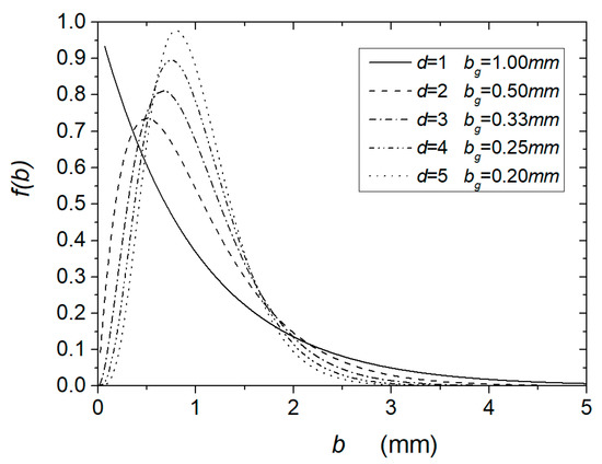
Figure 4. Gamma distribution pdf for different values of the parameter $d$ and assuming a mean fracture aperture $⟨b⟩=1$ mm.

4.2. Channels in Parallel

Inserting Equation (19) into Equation (9) gives the following result after integration [18] (p. 403), some algebraic manipulations, the use of Equation (20), and the exploitation of the properties of the gamma function:

$$q_x=\frac{AB⟨b⟩}{{\overline{P}}_x}{q}_{xD}; q_{xD}=\frac{1}{2\mathsf{\Omega }}\left[\frac{\left(d+1\right)u-1}{{\left(1-u\right)}^{d+1}}+\frac{\left(d+1\right)u+1}{{\left(1+u\right)}^{d+1}}\right],$$

(23)

where

$$\mathsf{\Omega }=\frac{\overline{P_x}⟨b⟩}{2A}=\frac{{\tau }_w}{A},$$

(24)

$$u=\frac{\mathsf{\Omega }}{d},$$

(25)

$$u<1_{.}$$

(26)

The relationships in Equations (24)–(26) establish that the ratio between the shear stress ${\tau }_w$ at the wall of a parallel-plate fracture of aperture $⟨b⟩$ and the characteristic shear stress $A$ describing the Prandtl–Eyring fluid cannot exceed the shape parameter $d$ of the aperture distribution. Figure 5 shows the dimensionless flow rate per unit width $q_{xD}$ as a function of $\mathsf{\Omega }$ for different values of $d$. It is seen that as $\mathsf{\Omega }\to 0^{+}$, the flow rate tends to $-\infty$; such negative values are obviously not realistic. On the other hand, for $\mathsf{\Omega }\to d$, the flow rate tends to infinity, and the curves show a vertical asymptote of the equation $\mathsf{\Omega }=d$. Similarly, such results are unrealistic. For low values of $\mathsf{\Omega }$, the curves tend to overlap, regardless of the value of $d$. In general, the flow rate depends, in a nonlinear fashion, on the dimensionless pressure gradient and the distribution parameters.

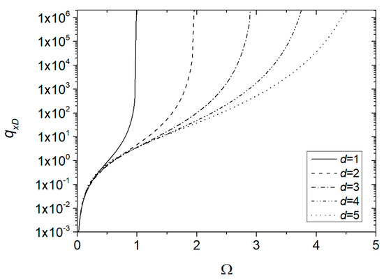
Figure 5. Dimensionless flow rate per unit width $q_{xD}$ versus dimensionless pressure gradient $\mathsf{\Omega }$ for different values of the distribution parameter $d$.

The hydraulic aperture for the parallel arrangement $b_{Hx}$ is obtained by solving the following implicit equation in the unknown $r_x$:

$$r_x\cosh \left(r_x\mathsf{\Omega }\right)-\frac{1}{\mathsf{\Omega }}\sinh \left(r_x\mathsf{\Omega }\right)=\frac{1}{2\mathsf{\Omega }}\left[\frac{\left(d+1\right)u-1}{{\left(1-u\right)}^{d+1}}+\frac{\left(d+1\right)u+1}{{\left(1+u\right)}^{d+1}}\right];r_x=\frac{b_{Hx}}{⟨b⟩}.$$

(27)

Figure 6 illustrates the ratio $r_x$ of the hydraulic to mean aperture defined by Equations (27) as a function of $\mathsf{\Omega }$ for different values of $d$. The ratio $r_x$ strongly increases with $\mathsf{\Omega }$, more so for lower values of $d$, i.e., a more skewed distribution. The curves show a vertical asymptote when the dimensionless pressure gradient $\mathsf{\Omega }$ approaches $d$. For low values of $\mathsf{\Omega }$, the curves are almost horizontal.

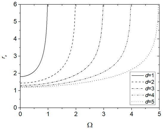
Figure 6. Ratio $r_x=b_{Hx}/⟨b⟩$ versus dimensionless pressure gradient $\mathsf{\Omega }$ for different values of the shape parameter $d$.

4.3. Channels in Series

The pressure gradient cannot be obtained explicitly as a function of flow rate from Equations (4) and (5) written by replacing the subscript $x$ with $y$; hence, the integral in Equation (16) with Equations (19)–(21) can only be solved numerically. Doing so yields $q_y=q_y\left(\overline{P_y},A,B, ⟨b⟩,d\right)$, which can be made dimensionless as $q_{yD}=q_{yD}\left(\mathsf{\Omega },d\right)$, where $q_{yD}$ is defined by Equation (23) with the subscript $y$ in place of $x$, and $\mathsf{\Omega }$ is defined by Equation (24).

The hydraulic aperture $b_{Hy}$ is obtained by solving the following implicit equation in the unknown $r_y$:

$$r_y\cosh \left(r\mathsf{\Omega }\right)-\frac{1}{\mathsf{\Omega }}\sinh \left(r\mathsf{\Omega }\right)=q_{yD}, r_y=\frac{b_{Hy}}{⟨b⟩}.$$

(28)

5. Comparison with Power-Law Fluid Flow

5.1. Results for a Power-Law Fluid

A power-law fluid has the rheological equation

$${\tau }_{zx}=-\tilde{\mu }{\left|\frac{d{v}_x}{dz}\right|}^{n-1}\frac{d{v}_x}{dz},$$

(29)

where $n$ is the rheological index, and $\tilde{\mu }$ is the consistency index of dimensions (ML⁻¹Tⁿ⁻²); for $n<1$ and $n>1$, the model describes shear-thinning (pseudoplastic) and shear-thickening (dilatant) behavior, whereas for $n=1$, Newtonian behavior is recovered, and $\tilde{\mu }$ reduces to dynamic viscosity $\mu$. The relationship between the applied pressure gradient $\overline{P_x}$ and flow rate per unit width $q_x$ in a parallel-plate fracture of aperture $b$ is

$$q_x=\frac{n}{2^{\frac{2n+1}{n}}\left(2n+1\right)}{\left(\frac{\overline{P_x}}{\tilde{\mu }}\right)}^{\frac{1}{n}}{b}^{\frac{2n+1}{n}}.$$

(30)

For the gamma distribution of an aperture defined by Equations (19)–(22), results are obtained after some algebra as

$$q_x={\left(\frac{\overline{P_x}}{\tilde{\mu }}\right)}^{\frac{1}{n}}{⟨b⟩}^{\frac{2n+1}{n}}{q}_{xD}, q_{xD}=\frac{n}{2^{\frac{2n+1}{n}}\left(2n+1\right)d^{\frac{2n+1}{n}}}\frac{\mathsf{\Gamma }\left[\left(\left(d+2\right)n+1\right)/n\right]}{\mathsf{\Gamma }\left(d\right)},$$

(31)

$$r_x=\frac{b_{Hx}}{⟨b⟩}={\left[\frac{\mathsf{\Gamma }\left[\left(\left(d+2\right)n+1\right)/n\right]}{\mathsf{\Gamma }\left(d\right)}\right]}^{\frac{n}{2n+1}},$$

(32)

$$q_y={\left(\frac{\overline{P_y}}{\tilde{\mu }}\right)}^{\frac{1}{n}}{⟨b⟩}^{\frac{2n+1}{n}}{q}_{yD}, q_{yD}=\frac{n}{2^{\frac{2n+1}{n}}\left(2n+1\right)d^{\frac{2n+1}{n}}}{\left[\frac{\mathsf{\Gamma }\left(d\right)}{\mathsf{\Gamma }\left(d-2n+1\right)}\right]}^{\frac{1}{n}},d>2n+1,$$

(33)

$$r_y=\frac{b_{Hy}}{⟨b⟩}={\left[\frac{\mathsf{\Gamma }\left(d\right)}{\mathsf{\Gamma }\left(d-2n+1\right)}\right]}^{\frac{1}{2n+1}} .$$

(34)

For a Newtonian fluid $\left(n=1, \tilde{\mu }=\mu \right)$ and a gamma distribution, results for parallel and serial arrangements reduce respectively to

$$q_x=\frac{\overline{P_x}}{\mu }{⟨b⟩}^3{q}_{xD}, q_{xD}=\frac{\left(d+1\right)\left(d+2\right)}{12d^2}, r_x={\left[\frac{\left(d+1\right)\left(d+2\right)}{d^2}\right]}^{\frac{1}{3}},$$

(35)

$$\begin{gathered} q_y=\frac{\overline{P_y}}{\mu }{⟨b⟩}^3{q}_{yD}, q_{yD}=\frac{\left(d-3\right)\left(d-2\right)\left(d-1\right)}{12d^3},r_y={\left[\frac{\left(d-3\right)\left(d-2\right)\left(d-1\right)}{d^3}\right]}^{\frac{1}{3}}, \\ d>3, \end{gathered}$$

(36)

while for a normal distribution $\left(d\to \infty \right)$ and a power-law fluid, one has

$$q_{xD}=q_{yD}=\frac{n}{2^{\frac{2n+1}{n}}\left(2n+1\right)}, r_x=r_y=1,$$

(37)

which further reduces for a Newtonian fluid to $q_{xD}=q_{yD}=1/12.$

5.2. Comparison between Power-Law and Prandtl–Eyring Models

In this section, the parallel arrangement is considered, and a comparison between the power-law and the Prandtl–Eyring models is proposed. Here, we aim to analyze the effects of a shear stress plateau in the Prandtl–Eyring model for low shear rates. The nature of a non-Newtonian fluid is hard to model, and this inevitably leads to a complex expression for the fluid rheology. The most commonly used model for a shear-thinning fluid is the power law relationship; it is a valid tool for studying non-Newtonian fluid behavior without introducing excessive mathematical complexities. It is, however, not entirely realistic, as for low shear rates ($\dot{\gamma }\to 0)$, the apparent viscosity tends to infinity ($\eta \to \infty$), while for ($\dot{\gamma }\to \infty )$, it results in $\eta \to 0$. The Prandtl–Eyring model is characterized by a viscosity upper bound; this rheologic model presents a plateau, and for $\dot{\gamma }\to 0$, the fluid resembles a Newtonian fluid with $\eta \to A/B$. To compare the two rheologies, a Prandtl–Eyring fluid ($A=0.003465 \mathrm{Pa}$ and $B=0.0231 {\mathrm{s}}^{-1}$) is considered [7] and adopted to evaluate the parameters of a comparable power-law fluid by means of a least-squares fit performed in the range of a shear rate between 10 and 1 × 10³ s⁻¹: the result of the best fit yields $\tilde{\mu }=0.0175 \mathrm{Pa}\times {\mathrm{s}}^n$ and $n=0.13$ (Figure 7).

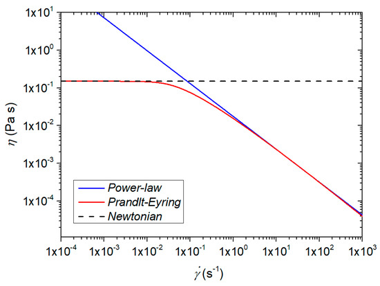
Figure 7. Plot of viscosity vs. strain rate: strain-rate viscosity form fit a Prandtl–Eyring rheology ($A=0.003465 \mathrm{Pa}$ and $B=0.0231 {\mathrm{s}}^{-1}$) of a power-law model ($\tilde{\mu }=0.0175 \mathrm{Pa}\times {\mathrm{s}}^n$ and $n=0.13$).

To analyze the influence of the plateau, we define the shear rate ratio ${⟨\dot{\gamma }⟩}_N/{⟨\dot{\gamma }⟩}_{PE}$, where ${⟨\dot{\gamma }⟩}_N$ is the average fracture shear rate of a Newtonian fluid of dynamic viscosity $\eta =A/B$, written as

$${⟨\dot{\gamma }⟩}_N={{\displaystyle \int }}_0^{+\infty }\left[\frac{1}{b}{{\displaystyle \int }}_{-\frac{b}{2}}^{\frac{b}{2}}\dot{\gamma }\left(z\right)dz \right]f\left(b\right)\mathrm{d}b=\frac{p_x⟨b⟩B}{4A},$$

(38)

and similarly, the average fracture shear rate of a Prandtl–Eyring fluid is

$${⟨\dot{\gamma }⟩}_{PE}=\frac{2ABd}{p_x\left(d-1\right)⟨b⟩}\left\{\frac{1}{2}\left[{\left(1-\frac{p_x⟨b⟩}{2Ad}\right)}^{1-d}+{\left(1+\frac{p_x⟨b⟩}{2Ad}\right)}^{1-d}\right]-1\right\}.$$

(39)

Figure 8 depicts the flow rate versus pressure gradient for power-law and Prandtl–Eyring fluids for channels in parallel within the range of validity (Equation (26)) of Equation (23). Both the red and blue solid lines, representing the Prandtl–Eyring and the power-law fluids, respectively, are monotonically increasing functions of the pressure gradient, with the former model showing a flow rate several orders of magnitude higher than the latter. The power-law model presents a linear trend in log-log coordinates, while two different behaviors can be observed in the Prandtl–Eyring model: for low-pressure gradients, the slope of the red solid line is minor compared with the one of the blue solid line but higher than the Newtonian case; on the other hand, when the average fracture shear rates of the two fluids are sufficiently different, the Prandtl–Eyring model rapidly increases its steepness. When the average fracture shear rates ${⟨\dot{\gamma }⟩}_{PE}$ tend to ${⟨\dot{\gamma }⟩}_N$, most of the channels undergo a flow regime of low shear rates, where the Prandtl–Eyring model simply resembles a Newtonian fluid of dynamic viscosity $\mu =A/B$.

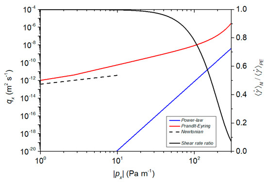
Figure 8. Plot of flow rate vs. pressure gradient; the red solid line represents the Prandtl–Eyring model ($A=0.003465 \mathrm{Pa}$ and $B=0.0231 {\mathrm{s}}^{-1}$), the blue solid line represents the power-law model ($\tilde{\mu }=0.0175 \mathrm{Pa}\times {\mathrm{s}}^n$ and $n=0.13$), and the black dashed line represents the Newtonian model ($\mu =A/B=0.15 \mathrm{Pa}\times s$). The plot of shear rate ratio ${⟨\dot{\gamma }⟩}_N/{⟨\dot{\gamma }⟩}_{PE}$ vs. pressure gradient is illustrated by the black solid line.

6. Conclusions

Non-Newtonian flow in a fracture characterized by an isotropic, two-dimensional aperture variation is complex; a simplified view is proposed that envisages the fracture as a random mixture of elements in which the fluid flows either transversal or parallel to a 1-D aperture variation, which is described by a probability distribution function of assigned mean and variance. The Prandtl–Eyring model was chosen to describe the fluid, as it captures the shear-thinning behavior of most fluids of interest in fractured media flow without the unrealistically large apparent viscosity for low shear rates typical of power-law fluids. The latter model was chosen for comparison. The gamma distribution was selected to represent aperture variability. Key results are as follows:

• Values of the flow rate are extremely sensitive to the applied pressure gradient and to the shape of the distribution; in particular, a more skewed distribution entails larger values of the dimensionless flow rate;
• A comparison was drawn between the Prandtl–Eyring (PE) and the power-law (PL) model having equal apparent viscosity for a wide range of shear rates. For channels in parallel, the absence of a shear stress plateau for low shear rates, associated with power-law rheology, implies an underestimation of the fracture flow rate with respect to the Prandtl–Eyring case. For the latter fluid, low-pressure gradients are characterized by a flow regime dominated by the plateau viscosity $\eta =A/B$, with a behavior similar to a Newtonian (N) fluid, while for sufficiently high-pressure gradients, as the ratio between the two average fracture flow rates (PE to N) increases, the effect of the falling limb of the Prandtl–Eyring model, associated with a lower apparent viscosity, becomes evident.

Future work will consider:

• the incorporation of drag effects, local losses, and slip in the simplified 1-D models;
• the adoption of truncated and correlated distributions to represent more realistically the spatial variability;
• further refinements of the fluid rheology (e.g., Powell–Eyring, Cross, or Carreau–Yasuda model [7]).

References

- Adler, P.M.; Thovert, J.F.; Mourzenko, V.M. Fractured Porous Media; Oxford University Press: Oxford, UK, 2002; p. 184. [Google Scholar]
- Wang, L.; Cardenas, M.B. Analysis of permeability change in dissolving rough fractures using depth-averaged flow and reactive transport models. Int. J. Greenh. Gas Control 2019, 91, 102824. [Google Scholar] [CrossRef]
- Meheust, Y.; Schmittbuhl, J. Geometrical heterogeneities and permeability anisotropy of rock fractures. J. Geophys. Res. 2001, 106, 2089–2102. [Google Scholar] [CrossRef]
- Silliman, S. An interpretation of the difference between aperture estimates derived from hydraulic and tracer tests in a single fracture. Water Resour. Res. 1989, 25, 2275–2283. [Google Scholar] [CrossRef]
- Lavrov, A. Redirection and channelization of power-law fluid flow in a rough walled fracture. Chem. Eng. Sci. 2013, 99, 81–88. [Google Scholar] [CrossRef]
- de Castro, A.R.; Radilla, G. Flow of yield stress and Carreau fluids through rough walled rock fractures: Prediction and experiments. Water Resour. Res. 2017, 53, 6197–6217. [Google Scholar] [CrossRef]
- Bechtel, S.; Youssef, N.; Forest, M.; Zhou, H.; Koelling, K.W. Non-Newtonian viscous oscillating free surface jets, and a new strain-rate dependent viscosity form for flows experiencing low strain rates. Rheol. Acta 2001, 40, 373–383. [Google Scholar] [CrossRef]
- Zimmerman, R.W.; Kumar, S.; Bodvarsson, G.S. Lubrication theory analysis of the permeability of rough-walled fractures. Int. J. Rock Mech. Min. Sci. Geomech. Abstr. 1991, 28, 325–331. [Google Scholar] [CrossRef]
- Yoon, H.K.; Ghajar, A.J. A note on the Powell-Eyring fluid model. Int. Commun. Heat Mass 1967, 14, 381–390. [Google Scholar] [CrossRef]
- Rehman, K.U.; Awais, M.; Hussain, A.; Kousar, N.; Malik, M.Y. Mathematical analysis on MHD Prandtl-Eyring nanofluid new mass flux conditions. Math. Methods Appl. Sci. 2019, 42, 24–38. [Google Scholar] [CrossRef]
- Bear, J. Dynamics of Fluids in Porous Media; Elsevier: New York, NY, USA, 1972; p. 764. [Google Scholar]
- Di Federico, V. Estimates of equivalent aperture for Non-Newtonian flow in a rough-walled fracture. Int. J. Rock Mech. Min. Sci. Geomech. Abstr. 1997, 34, 1133–1137. [Google Scholar] [CrossRef]
- Brown, S.R. Transport of fluid and electric current through a single fracture. J. Geophys. Res. 1989, 94, 9429–9438. [Google Scholar] [CrossRef]
- Di Federico, V. Non-Newtonian flow in a variable aperture fracture. Transp. Porous Med. 1998, 30, 75–86. [Google Scholar] [CrossRef]
- Felisa, G.; Lenci, A.; Lauriola, I.; Longo, S.; Di Federico, V. Flow of truncated power-law fluid in fracture channels of variable aperture. Adv. Water Resour. 2018, 122, 317–327. [Google Scholar] [CrossRef]
- Zimmerman, R.W.; Bodvarsson, G.S. Hydraulic conductivity of rock fractures. Transp. Porous Med. 1996, 23, 1–30. [Google Scholar] [CrossRef]
- Dagan, G. Flow and Transport in Porous Formations; Springer: Berlin/Heidelberg, Germany, 1989; p. 658. [Google Scholar]
- Gradshteyn, I.S.; Ryzhik, I.M. Table of Integrals, Series, and Products; Academic Press: New York, NY, USA, 1994; p. 1204. [Google Scholar]
© 2020 by the authors. Licensee MDPI, Basel, Switzerland. This article is an open access article distributed under the terms and conditions of the Creative Commons Attribution (CC BY) license (http://creativecommons.org/licenses/by/4.0/).