Abstract
Stochastic simulation has a prominent position in a variety of scientific domains including those of environmental and water resources sciences. This is due to the numerous applications that can benefit from it, such as risk-related studies. In such domains, stochastic models are typically used to generate synthetic weather data with the desired properties, often resembling those of hydrometeorological observations, which are then used to drive deterministic models of the understudy system. However, generating synthetic weather data with the desired properties is not an easy task. This is due to the peculiarities of such processes, i.e., non-Gaussianity, intermittency, dependence, and periodicity, and the limited availability of open-source software for such purposes. This work aims to simplify the synthetic data generation procedure by providing an R-package called anySim, specifically designed for the simulation of non-Gaussian correlated random variables, stochastic processes at single and multiple temporal scales, and random fields. The functionality of the package is demonstrated through seven simulation studies, accompanied by code snippets, which resemble real-world cases of stochastic simulation (i.e., generation of synthetic weather data) of hydrometeorological processes and fields (e.g., rainfall, streamflow, temperature, etc.), across several spatial and temporal scales (ranging from annual down to 10-min simulations).
1. Introduction
“Oh, Lord, please keep the world linear and Gaussian.”~ Chester Kisiel’s [1] pray to the theoretical hydrologist [2] (p. 288).
1.1. Motivation
The notions of stochastics and randomness have a prominent position in a variety of scientific fields, such as those of biology, finance, artificial intelligence, environmental and water resources science, as well as hydrology. This is due to the ability offered by the relevant mathematical objects, such as those of random variables, stochastic processes, and random fields, to provide the basis to account for uncertainty in the analysis and modeling of physical or non-physical systems. Characteristic applications are risk- or reliability-based studies which typically aim to propagate the uncertainty of the inputs into the outputs of interest, and eventually into the decision-making procedure (formulating a type of Monte-Carlo experiments). For instance, this rationale has been widely employed in the domain of environmental and water resources science where, apart from providing tools to simulate hydrometeorological processes per se, stochastic models are used to provide synthetic inputs with the desired properties (typically resembling those of observed processes, e.g., hydrometeorological ones) to drive physically- or conceptually-based (typically deterministic) models of the system under study. See for instance the works of Koutsoyiannis and Economou [3], Celeste and Billib [4], Haberlandt et al. [5], Giuliani et al. [6], Tsoukalas and Makropoulos [7,8], Tsoukalas et al. [9], Feng et al. [10], and Do and Razavi [11] in environmental and water resources domain, as well as the works Robert and Casella [12] and Kroese et al. [13,14] for other applications in science and real-word practice.
At this point, it is noted that, for the sake of simplicity (although not being entirely precise), throughout the paper, we may use the term stochastic process to refer also to random variables (RVs) and random fields (RFs).
Despite the wide use of stochastic modeling approaches, it is generally acknowledged that generating synthetic inputs with the desired properties is not an easy, nor a standardized task. In our view, this can be mainly attributed to two reasons associated with: (1) the deviation from Gaussianity exhibited by several physical and non-physical processes (e.g., [15]); and (2) the limited availability of general, easy-to-use, open-source software designed for such purposes (see the relevant discussion by Efstratiadis et al. [16]). The first point is evidently related with the introductory aphorism of this paper (i.e., Chester Kisiel’s pray to the theoretical hydrologist), which reflects the generally challenging task of handling non-Gaussian behavior, especially for hydrometeorological processes, which, beyond non-Gaussianity, are also characterized by other significant peculiarities such as intermittency, auto- and cross-dependence and periodicity [17,18,19]. These characteristics are also apparent in other types of processes (e.g., non-physical ones such as water demand processes; see Kossieris et al. [20]).
In our view, it is argued that the primary difficulty in the modeling of such characteristics originates from the fact that the classical linear stochastic models were formally developed for the simulation of correlated Gaussian random variables, processes, and fields - a fact that hampers their use (without modifications; e.g., see the relevant discussion in Tsoukalas et al. [21,22]) in a wide range of real-world applications that involve processes that deviate significantly from Gaussianity.
1.2. Modeling Rationale and Historical Overview
The need for suitable non-Gaussian models have motivated many research efforts in a variety of scientific domains, particularly in the hydrological one (e.g., see [5,23,24,25,26,27,28,29,30] for relevant discussions, model classifications and reviews). These efforts can be coarsely classified into two groups [31]. The first group regards methods that aim to resemble a process in terms of summary statistical characteristics, such as moments (e.g., mean, variance, and skewness) and (typically low-order) correlation coefficients (e.g., [16,32,33,34,35,36,37,38,39] (pp. 53–57) [40,41,42,43,44,45]). The second group consists of methods that aim to simulate realizations of a process with target marginal distributions and correlation structures. In the present work, we focus on methods of the second group since by definition provide a more accurate modeling approach (for further arguments, see Deodatis and Micaletti [31], as well as Tsoukalas et al. [25] and references therein). At the same time, these methods avoid a problem called envelope behavior encountered in popular stochastic simulation approaches (i.e., based on the rationale of Thomas and Fiering model) of the first group; a problem that regards the generation of time series with unrealistic dependence patterns [22].
Particularly, here, we focus on methods that rely on the so-called Nataf’s joint distribution model [46]. A concept that was initially proposed for the simulation of correlated RVs [47,48], yet, as discussed next and detailed in Section 2.3, can and has been employed also for the simulation of non-Gaussian stochastic processes and random fields.
Nataf’s joint distribution model (NDM) suggests that the joint distribution of correlated random variables (RVs) with any target marginal distributions can be obtained on the basis of an appropriately parameterized auxiliary multivariate standard Gaussian distribution, and specifically by mapping the correlated Gaussian variables to the target distributions via their inverse cumulative distribution function (ICDF). It is also interesting to note that NDM is essentially what we call today a Gaussian copula [49].
As literature reveals, the notion of NDM has been used in several disciplines for the simulation of non-Gaussian RVs, stochastic processes and RFs, but under many different names (see an earlier, yet relevant, discussion in Section 4.6 of Tsoukalas et al. [21] which regards applications of NDM in hydrological domain). Indicatively, we note that the notion of NDM, a term widely used in the domain of structural and civil engineering [47,50,51,52,53,54], is similar with concepts used in other scientific domains, such as those of, non-linear (often called memoryless) transformation approaches [55,56,57,58], translation processes [15,59,60], meta-Gaussian approaches [61,62,63], latent Gaussian processes [64,65,66,67], transformed Gaussian processes [68,69,70,71], parent Gaussian methods [72,73,74], and the so-called To-Anything approaches [20,21,25,75,76,77,78,79,80].
A closer look at the above research efforts reveals that all those methodologies share a common element that is the mapping (transformation or translation) of a (auxiliary, latent ore parent) Gaussian vector, process or field to the desired domain via a non-linear function (typically the ICDF) to obtain correlated RVs, stochastic processes, and RFs, respectively, with target marginal distributions and correlation structure. Therefore, it can be argued that all rely on the concept of NDM. It is also noted that several of these methods aim to resemble a process with a prescribed spectrum instead of correlation structure, which is of course equivalent since the correlation and spectrum are interrelated quantities (e.g., see the spectrum-based works of Yamazaki and Shinozuka [81] and Deodatis and Micaletti [31]). It should be pointed out that the preservation of the target correlation structure (after the mapping) is directly linked with the appropriate parameterization of the underlying Gaussian model on the basis of the so-called equivalent correlation structure (see Section 2.2), a delicate step often neglected.
To elaborate more, NDM was employed by Li and Hammond [82], van der Geest [83], and Cario and Nelson [75], under the term NORmal To Anything (NORTA), for the generation of correlated non-Gaussian RVs, extending it also for random vectors with continuous and discrete marginal distributions, as well as combinations of them. In the same spirit, Kelly and Krzysztofowicz [61] used a bivariate Gaussian distribution to establish the so-called bivariate meta-Gaussian distribution that can admit arbitrarily specified marginal distributions. See also the relevant works on the topic by Moran [40], who focused on the case of a bivariate Gamma distribution, and Emrich and Piedmonte [84], who studied a method for the generation of multivariate binary variates.
Moving beyond random variables, the concept of NDM has been employed for the simulation of non-Gaussian stochastic processes in a similar way to RVs. In this modeling case, an auxiliary Gaussian process with zero mean and unit variance (e.g., simulated via linear stochastic models, such as autoregressive moving average (ARMA) models) is mapped to the target domain. The development of such modeling techniques can be traced back to the early works of Gujar and Kavanagh [85], Klemeš and Borůvka [86], and Matalas [32], as well as the seminal work of Grigoriu [59], who also referred to the notion of NDM, and the relevant sequel works [15,60] that adopt the term translation process. In a similar vein, Cario and Nelson [76] developed the AutoRegressive To Anything (ARTA) model that combines an autoregressive linear model with NDM to simulate auto-correlated univariate stationary processes with any marginal distribution. Further to this, ARTA model was later further extended for multivariate simulations by the Vector AutoRegressive To Anything (VARTA) approach [80]. In this spirit, Tsoukalas et al. [21,77] developed the Stochastic Periodic AutoRegressive To Anything (SPARTA) scheme that is a generalization of ARTA and VARTA models for the simulation of univariate and multivariate cyclostationary (i.e., periodic) processes with arbitrary marginal distributions. Furthermore, the Symmetric Moving Average To Anything (SMARTA) model [78] combines NDM with the symmetric moving average model [44] to simulate non-Gaussian processes that exhibit any-range dependence structure. Analogously, Papalexiou [72], using autoregressive models, proposed an approach for the stochastic modeling of hydroclimatic processes, with focus on the modeling intermittency. Further to these, recent developments [25,79] offer modular multivariate stochastic simulation schemes that can generate multi-scale consistent time series at multiple locations (or of multiple processes at the same location). A modeling task of high importance in water resources applications [16,43,87,88].
Moving to random fields (RFs), their modeling and simulation has been for years an active topic of research with contributions spanning across theoretical developments [89,90,91], as well as earth science applications (e.g., [58,71]). RFs offer the tools to mathematically describe a wide range of processes (e.g., hydrometeorological) accounting for both spatial and temporal dynamics. The literature offers a variety of methods for such modeling task (see the above-referenced works), yet most of them concern Gaussian RFs and methods focusing on the spatial dynamics. In this vein, and for reasons mentioned above, herein we turn our focus on non-Gaussian methods that rely on the concept of NDM. A literature review reveals that the NDM concept has been widely employed for the simulation of non-Gaussian RFs [50,51,52,55,56,57,58,63,67,70,73,81,92], but again different names were adopted. Indicatively, we mention the works of Bell [68] and Lanza [69] who devised a model for the simulation of rainfall’s random fields through the transformation of a Gaussian field to a non-Gaussian one, characterized by a zero-inflated log-Normal marginal distribution (to account for rainfall’s intermittent behavior). In the same spirit, Rebora et al. [55] used a static non-linear transformation to map a Gaussian RF to log-Normal distribution, while similar approaches can be found in the works of Christakos [58] and Gong et al. [70]. Other approaches, termed meta-Gaussian or latent Gaussian, were employed by Guillot [63], Guillot and Lebel [62], and Baxevani and Lennartsson [67], who also used the notion of auxiliary (or latent) Gaussian RFs that are subsequently mapped to the target domain via a non-linear transformation. See also the work of Gioffrè et al. [92], who used translation-based method for the simulation of non-Gaussian fields of wind pressure fluctuations. Finally, a more recent treatment that regards the simulation of hydrometeorological RFs was given by Papalexiou and Serinaldi [73] who used the term parent-Gaussian fields.
1.3. Contribution and Organization of the Paper
Currently, there is a strong momentum in the development of Nataf-based schemes in the realm of environmental science, water resources and hydrology since such methods have been proven capable of simulating processes with characteristics exhibited in both physical (e.g., rainfall, streamflow, and wind) and non-physical (e.g., water demand) processes [20,21,25,72,73,77,78,79,93]. In this spirit, and aiming to fulfill the need for general and open-source software for synthetic data generation, this work builds upon this momentum, as well as past research efforts, and presents an R package called anySim. This endeavor aims to facilitate the easy simulation of non-Gaussian correlated random variables, stochastic processes, and random fields, providing this way the means to practitioners and researchers to easily access and employ state-of-the-art stochastic simulation methods, required by a variety of uncertainty-aware frameworks and analyses (e.g., risk-based engineering studies).
The remaining of this paper is structured as follows. Section 2 presents a brief introduction to the key aspects of the NDM approach, providing also simple guides and technical details for the development of NDM-based stochastic simulation schemes. Section 3 describes the structure, modules, and functionalities of the developed anySim R-package. Section 4 presents a suite of simulation problems focused on the stochastic simulation of hydrometeorological processes (e.g., rainfall, streamflow, temperature, etc.), demonstrating the functionalities of the package and the associated models, while Section 5 provides the simulation results of the demonstration problems, as well as the associated R-code (i.e., a tutorial). Finally, Section 6 concludes this work, highlighting also interesting future research activities to improve the functionalities and utility of anySim. It is noted that a reader familiar with the rationale of NDM and the related methods could skip Section 2 and go directly to Section 3, Section 4 and Section 5 where the anySim package is detailed and demonstrated.
1.4. A Brief Note on Notation and Style Used
In general, throughout this manuscript, we refer to a function (either distribution function or correlation structure) by writing its name followed by a parenthesis containing the corresponding R-function using Courier New fonts. For instance, the ICDF of the Gamma distribution (qgamma). Moreover, and unless stated otherwise, regarding distribution functions, we typically use the Greek letters and to denote the distribution’s shape and scale parameters, respectively, as well as the letter to denote the location parameter. In the case of more than one shape parameter, we use the same letter using subscripts (e.g., and). Furthermore, we use (intuitively-chosen) script letters to abbreviate distributions, e.g., a random variable that follows the Gamma distribution is denoted by .
2. Methods
2.1. Theoretical Background of NDM Approach
As discussed in the previous section, the NDM approach, after certain extensions and modifications, can be applied for the simulation of correlated random variables, stochastic processes, and random fields. Although anySim supports all these modeling applications, here we choose to present the key theoretical aspects of Nataf-based schemes on the basis of a problem that studies the generation of two random variables with predefined marginal distributions and correlation. This bivariate simulation problem describes the simplest simulation scenario but is the cornerstone of any Nataf-based approach (e.g., that could regard stochastic processes or random fields) since the linear stochastic models (that are used to establish the auxiliary Gaussian process or field) are also based on Pearson’s correlation coefficient which is a two-point dependence measure. The interested reader may also refer to Tsoukalas et al. [78] and Tsoukalas et al. [21,25] for alternative descriptions of the theoretical background of NDM approach on the basis of multivariate stationary and cyclostationary stochastic processes, respectively.
Back to the bivariate simulation case, let us assume that our target is to generate correlated random variables (RVs) and with predefined target marginal distributions and , respectively, and target correlation , which stands for the Pearson’s correlation coefficient between the two variables, hereinafter abbreviated as .
Let us initially define two auxiliary correlated RVs and , which both have the standard Gaussian marginal distribution and correlation coefficient , herein after termed as equivalent correlation (for reasons explained below) and abbreviated as . It is noted that the joint distribution of the two auxiliary variables is the bivariate Gaussian with zero mean, unit variance, and correlation .
The target RVs and can be obtained by mapping the auxiliary normal variables to the target distributions via the following mapping operations:
where and denote the inverse cumulative distribution functions (ICDF) of the target distributions of and , respectively, and stands for the standard Gaussian cumulative distribution function (CDF).
Since the mapping procedure presented in Equation (1) is based on the ICDF of the target distribution, it ensures by construction that the final variables will have the desired marginal properties. On the other hand, the use of ICDF imposes a nonlinear and monotonic transformation, and hence this mapping does not ensure the preservation of the linear correlation coefficients [94]. Specifically, the sole use of this mapping operation leads to typically reduced correlation coefficients, while as the target distribution deviates from the Gaussian case, the larger will be the reduction. However, it can be shown the equivalent correlation and the target one are linked by [47],
where and denote the mean and variance of the known target distributions, is the standard bivariate Gaussian probability density function (PDF) with correlation . The latter equation can be compactly expressed as,
where is the abbreviation of the function defined in Equation (2). Therefore, the key challenge in any NDM approach is to determine the equivalent correlation that will result to the target correlation , after applying the mapping procedure (i.e., determine the link between and ). This operation can be accomplished by inverting Equation (3) that can be compactly written as,
Further details on the relationship among the equivalent and target correlation coefficients, both of practical and theoretical interest, can be found given in several works in the related literature (e.g., [21,47,72] and references therein), while interesting discussions on its theoretical bounds were provided by Fréchet [95],Whitt [96], Hoeffding [97], and Armstrong [98]. The interested reader is also referred to [99] and [100], where the authors using entropy-related notions, provided an alternative view, as well as useful insights on the topic.
2.2. Establishing Target-Equivalent Correlation Relationship
In the general case, the establishment of the target-equivalent correlation relationship requires the use of numerical schemes and integration methods [21,72,76,82,101,102], since the relationship in Equation (3) has analytical solution only for a few cases, for instance, when the marginal are uniform [82,103] or log-Normal [32,104,105]. It is also noted that the use of alternative rank-based dependence quantities, such as the Kendall’s tau and Spearman’s rho, should be avoided for the estimation of , since the relationships [49,106,107] that link those quantities assume that the marginal distributions are Gaussian, which is rarely the case (see the discussion in Tsoukalas [79] Section 4.5.3 and Tsoukalas et al. [78] Section 3.2.3).
In anySim, aiming to simplify the establishment of the target-equivalent correlation relationship, we have automated this procedure via a function called NatafInvD. In brief, this function avoids the use of iterative methods (in the sense of [81]) and works as follows (further details can also be found in the manual of the package): Equation (3) is solved (e.g., via Monte-Carlo or an integration method) for a specific set of values, and the corresponding target values are obtained. Then, an approximation function (either a polynomial or a parametric one) is fitted to these known anchor points, establishing an approximation of the true . The equivalent correlation , given a target correlation, is obtained by inverting the fitted function. Regarding the first step, the user can choose between three integration methods by providing appropriate values (in the form of a string) in the argument NatafIntMethod of NatafInvD. The integration methods supported are Gauss–Hermite integration (GH), adaptive multidimensional integration (Int), and Monte-Carlo integration (MC). Regarding the second step, polydeg argument of NatafInvD is a scalar indicating the order of the fitted polynomial, while, if polydeg = 0, then the function fits an alternative and simpler two-parameter function (see [72]). It is noted that the “MC” method (see [21]) captures the whole form of and is applicable irrespective of the type of marginal distributions (i.e., continuous, discrete or mixed-type of distributions), hence recommended when the target marginals are discrete.
2.3. Developing Nataf-Based Stochastic Simulation Schemes
In the modeling and simulation of stochastic processes and random fields, key requirements are the reproduction of both the marginal behavior (i.e., target distribution function) and dependence structures both in time and in space, as expressed by the auto- and cross-correlation coefficients, respectively. In this vein, a key component of any Nataf-based simulation scheme is the Gaussian process (Gp) model that generates the auxiliary realizations (in analogy to the auxiliary Gaussian RVs as presented in Section 2.1), which are then mapped to the target distribution of the non-Gaussian process via the ICDF.
The role of the model that simulates the Gaussian process is crucial in the whole procedure since its structure determines that of the target process, e.g., to simulate a stationary auto-correlated process then a stationary Gaussian process should be employed, while the simulation of a cyclostationary one requires the use of an auxiliary cyclostationary Gaussian model. It is important to highlight that, irrespective of this choice, the Gaussian model should be parameterized on the basis of equivalent correlation coefficients. This implies that the auxiliary realizations will preserve the equivalent correlation coefficients, ensuring (after their mapping via the ICDF) the reproduction of target auto- and cross-correlation structures. Note that the selection of the stochastic simulation model for the generation of auxiliary Gaussian realizations (e.g., via spectra-based methods that use trigonometric series, covariance decomposition methods or linear stochastic models such as ARMA models) is merely a matter of modeling requirements and convenience.
An option adopted in this work and implemented in anySim package is the use of Gaussian linear stochastic models (often called ARMA models). In this respect, the widely-known stationary autoregressive model of order (AR()), in a univariate or multivariate context, can be employed in the case of stationary processes. An alternative option is offered by the univariate or multivariate Symmetric Moving Average model of order (SMA()), introduced by Koutsoyiannis [44]. In the case of cyclostationary processes, i.e., when the distribution function and correlation structure of the process vary periodically from season-to-season, any stochastic scheme from the family of standard periodic autoregressive model of order (PAR()) could be used. For the sake of simplicity and parsimony, anySim focuses on the univariate and multivariate contemporaneous PAR(1) model [108] that supports the reproduction of season-to-season lag-1 correlations as well as the lag-0 cross-correlations among processes. Especially for most of practical applications in hydrology, it is argued that this model suffices, keeping the number of parameters to a minimum [43] (provided that the process at the temporal scale of simulation is characterized by cyclostationary, e.g., monthly runoff).
Regarding the stationary auxiliary AR() or (SMA()), as a side note, we remind that the use of high values of or q does not comes at the cost of parsimony of the relevant Nataf-based schemes, since in anySim we also employ the concept of theoretical (auto) correlation structures (see also Section 2.5). In this vein, the theoretical structure completely determines the autocorrelation structure of the target process, while the order or q of the models essentially determines the maximum time lag up to which the target structure will be reproduced. Having said this, the parameters of the AR or SMA models are simply regarded as internal coefficients, to be estimated from the target autocorrelation structure [25,44,78].
With respect to the above and the procedure briefly described in Section 2.1, a general framework for the establishment of Nataf-based schemes for the stochastic simulation of non-Gaussian processes (univariate or multivariate) and random fields is briefly described in Section 2.3.1 and Section 2.3.2, respectively.
2.3.1. A Layman’s Step-by-Step Guide for the Simulation of Non-Gaussian Processes
Step 1. Identify the type (i.e., stationary or cyclostationary, univariate or multivariate) of the processes, accounting for the process’ properties and the time scale of simulation.
Step 2. Based on the available information (e.g., historical data), as well as the user expertise, assign appropriate target marginal distributions for the processes and identify the target correlation structure, in time and space (in the case of multivariate simulation). For more details, see Section 2.5.
Step 3. Select a suitable stochastic model to simulate the auxiliary Gaussian process (Gp), based on the analysis of Step 1.
Step 4. Estimate the equivalent correlation coefficients for all pairs of interest, which are required by the parameter estimation procedure of the auxiliary Gp model.
Step 5. Estimate the parameters of the auxiliary Gp model using the equivalent correlation coefficients.
Step 6. Generate a synthetic Gaussian time series by employing the auxiliary Gp model.
Step 7. Map the auxiliary Gaussian time series to the actual domain (using the target ICDF) in order to attain a realization of the target process.
2.3.2. A layman’s Step-by-Step Guide for the Simulation of Non-Gaussian Random Fields
Step 1. Identify the type (i.e., spatial or spatiotemporal) of the RF to simulate, accounting also for its properties and the time scale of simulation.
Step 2. Based on the available information (e.g., gridded historical data or satellite observations), as well as the user expertise, assign an appropriate target marginal distribution for the RF and identify the target correlation structure, in time and space (for more details, see Section 2.5).
Step 3. Select a suitable stochastic model to simulate the auxiliary Gaussian RF, based on the analysis of Step 1.
Step 4. Estimate the equivalent correlation coefficients for all pairs of interest, which are required by the parameter estimation procedure of the auxiliary Gaussian RF model.
Step 5. Estimate the parameters of the auxiliary Gaussian RF model using the equivalent correlation coefficients.
Step 6. Generate a synthetic Gaussian RF by employing the auxiliary Gaussian RF model.
Step 7. Map the auxiliary Gaussian RF to the actual domain (using the target ICDF) in order to attain a realization of the target RF.
It is noted that, for the sake of convenience, the above guide regards the simulation of homogenous, stationary, and isotropic RFs, yet it can be easily adopted to account for anisotropy and cyclical stationarity. Particularly, the former one can be accomplished by using either appropriate coordinate transformation functions (e.g., [109]) or by directly employing anisotropic correlation structures [58,110,111], while the latter one by cyclically varying the parameters of the marginal distribution and those determining the process’ spatiotemporal correlation structure.
Based on the two above guides, anySim implements a great variety of Nataf-based schemes, capable of simulating a wide range of non-Gaussian processes and fields. These schemes along with the corresponding R-functions are presented in Section 3.2.
2.4. Multi-Scale Stochastic Simulation Via Disaggregation
Another modeling application supported by anySim package is the multi-scale stochastic simulation that targets the simultaneous reproduction of the marginal and stochastic behavior of processes across multiple temporal levels. It is well known that multi-scale consistency cannot be achieved via single-scale simulation since the reproduction of the characteristics of the process at a specific spatiotemporal level (expressed in terms of either a distribution function or a set of statistical characteristics) does not ensure the resemblance of the relevant characteristics of the aggregated process at any higher spatiotemporal level.
The problem of multi-scale consistency holds a prominent position in the modeling of hydrometeorological processes and it is of high practical interest since the effect of statistical and stochastic properties of synthetic series, which are used as inputs in a system model may extend far beyond the scale of simulation of the system [112].
The multi-scale simulation schemes are typically based upon the concept of disaggregation. According to this concept, the synthetic series are generated with the requirement to reproduce the characteristics of the process at a finer scale (e.g., monthly scale) and, simultaneously, to be fully consistent with the given data of a coarser scale (e.g., annual scale). The full consistency between the series of two time scales implies that the additive property is preserved at any period, i.e., the lower-level variables within each period sum up exactly to the given higher-level total for this period.
The hydrological literature offers several methods for such purposes (i.e., multi-scale simulation and/or disaggregation), yet few of them are freely available in R. For instance, CastaliaR [113] is a solution based on linear stochastic models with non-gaussian white noise (see also [16]), while HyetosMinute (see [114] and references therein) makes use of the Bartlett–Lewis clustering mechanism for the simulation of rainfall at fine time scales. Moreover, it is noted that both solutions aim at the preservation of the process moments, and not its distribution. On the contrary, anySim aims at the preservation of the process marginal distribution and correlation structure via using an approach based on multi-scale simulation via disaggregation. Specifically, anySim implements the so-called Nataf-based Disaggregation to Anything (NDA) framework ([25]; see also the brief discussion on alternative methods). NDA consists a scale-free disaggregation approach for the pairwise coupling of Nataf-based schemes, each applied individually to simulate the process at a coarser and finer time scale. A key element of this approach is a mathematical transformation, termed as adjusting procedure, which is applied to the lower-level series (e.g., monthly) to establish full consistency, i.e., preservation of the additive property, with the series of the higher-level (e.g., annually). Additionally, NDA incorporates a Monte Carlo-type repetitive sampling procedure to ensure that the sum of the independently generated lower-level series are close to the given higher-level values, establishing an a priori consistency between the two series and improving in this way the efficiency of the method. These two key elements are thoroughly discussed by Koutsoyiannis and Manetas [43] and Koutsoyiannis [88].
NDA can be employed for both multivariate and univariate multi-temporal simulation, after certain modifications and appropriate selection of a Nataf-based scheme, depending on the characteristics of the process studied (see previous section). Here, to keep things simple, we briefly present the whole procedure on the basis of a problem that studies the disaggregation of a univariate coarser-level series to a lower-level one.
Given that a realization , of a process , where is the time index, is known at a specific time scale (the coarser temporal level), we aim to produce fully consistent lower-level realizations of a process , with denoting the time index at the lower scale. Let also equal to the ratio of the time units of higher-level to the time units of lower-level (e.g., 1-year/1-month = 12, 1-day/1-h = 24, 1-day/1-min = 24 × 60, etc.). The coarser-level realization is known either from observations or it has been generated by another model. The disaggregation procedure applied for all time indices is the following:
Step 1. Using a Nataf-based model, generate temporary realizations of the lower-level process , of length .
Step 2. Aggregate (e.g., using the sum operator) the lower-level temporary realizations to obtain the higher-level temporary realizations i.e.,
Step 3. Estimate the distance , where , between the temporary realizations and the given one via an appropriate distance metric.
Step 4. Select the temporary realization , whose corresponding aggregated value (i.e., ) has the minimum . The selected lower-level realization is hereafter denoted as , and its corresponding aggregated value is denoted by
Step 5. Produce the final synthetic realizations by modifying the selected temporary realization via an adjusting procedure that allocates the difference between the given realization and the sum of the selected auxiliary realizations, .
As presented in detail in Section 3.2, anySim currently supports the disaggregation of univariate coarser-level processes to stationary or cyclostationary processes.
As a distance metric (Step 3) to quantify the consistency between the temporary and the given coarser level realizations, anySim employs the simple squared difference between and ; while the consistency between the selected realization and the given higher-level realization (Step 5) is established using the so-called proportional adjusting procedure, which is mathematically defined by
2.5. Technical Details
As discussed above, the simulation schemes implemented in anySim can be used in combination with any marginal distribution function (with such parameters that ensure finite variance) and valid (i.e., positive definite) correlation structures, describing either the temporal or spatial dependence of the process/field. In this section, we provide technical details on the marginal distribution functions and correlation structures, which are used in the simulation studies examined next, consisting though generic modeling paradigms.
2.5.1. Marginal Distributions
The flexibility provided by NDM to employ any marginal distribution allows one to use any continuous, discrete, or mixed-type distribution, given that it is parameterized to have finite variance. A list of distribution functions (continuous and discrete) employed in this work is given in Appendix A, while here we briefly discuss the case of zero-inflated () marginal distribution (also known as, zero-augmented or discrete-continuous). is a two-component (one discrete and one continoous) mixed-type distribution function holding a prominent position in hydrology since it can parsimoniously describe intermittent processes, such as rainfall and streamflow at fine time scales [25,68,69,72,78,115,116,117,118,119,120]. The CDF, denoted as (pzi), and ICDF, denoted as (qzi), of the zero-inflated distribution are given, respectively, by,
where is a parameter controlling the inflation of zeros (i.e., the discrete part of the distribution – the probability of observing zero values) and denotes the distribution to be inflated (i.e., the continuous part of the distribution). The combination of this distribution with Nataf-based models for simulating intermittent processes (i.e., rainfall) was recently formalized in [72], as well as employed by other works [20,25,78,79]. Earlier hydrology-related applications that couple Nataf-based schemes (although not recognized as such at the time) with this distribution model can found in the works of Bell [68] and Lanza [69] conducted in 1987 and 2000 respectively, who used a zero-inflated distribution in combination with a the log-Normal one for the continuous part. Further details on the distribution can be found in the work by Aitchison [121], as well as that of Kedem et al. [120], who among others provided the relationships that give its product moments. It is also noted that the model can be combined with a two-component mixture distribution for the description of the continuous part of the process, enabling the distinct modeling of the main body and the tail behavior of the distribution [20,93].
In the following simulation examples (Section 4 and Section 5), for notation convenience, we refer to such distribution using the prefix followed by the abbreviation of the continuous distribution, while the parameters of the model will be also provided in the followed parenthesis. For instance, a zero-inflated Gamma distribution (abbreviated by with parameters shape and scale ) is referred to as .
2.5.2. Correlation Structures
Further to marginal distributions, anySim currently implements three correlation structures (CSs), i.e., , where a is an index that could denote either the separation distance (typically Euclidean) of two points in space (hereafter, we use the letter for that case) or the time lag (in this case, we use the letter ). In the former case, we refer to it as the cross-correlation structure (CCS; i.e., spatial) of the process, while in the latter as the auto-correlation structure (ACS; i.e., temporal).
The following description of the three CSs implemented in anySim, and the corresponding notation (i.e., the use of index ), is oriented towards the representation of the ACS of a process, yet we remark that the same models can be also employed for the representation of spatial dependencies (i.e., cross-correlation) by using instead of , an index (see Section 5.5 for an example).
The first CS implemented in the package is the so-called two-parameter Cauchy-type correlation structure (CAS; cscas), introduced by Koutsoyiannis [44] as an ACS, which is able to capture a wide range of processes. CAS is given by:
where and are model parameters, and denotes the time lag. It is noted that depending on the values of its parameters CAS can model both short- () and long-range () dependence, i.e., SRD and LRD, respectively [16,20,25,44,78].
The second CS is that of the Hurt–Kolmogorov (HK; csHurst) process, or else known as fractional Gaussian noise (fGn) process [122,123,124,125,126], whose form is given by:
where H is a parameter (0 ≤ H ≤ 1), called Hurst coefficient, determining the extent of LRD. It is remarked that, under certain parameterization, CAS can provide an accurate approximation of fGn CS [44]. For further details, the interested reader is referred to the aforementioned work, as well as in the broader literature, mainly focusing on temporal LRD processes, which as it is argued are omnipresent in nature [124,127,128,129].
The third CS contained in anySim, typically used only as an ACS, is a simple periodic function (csPeriodic) given by MacKay [130]:
where and are parameters, denoting the distance among function’s repetitions and the process’s length scale, respectively. This function is particularly useful in the modeling of stationary processes with periodically varying autocorrelation coefficients, since it can be easily combined (though multiplication) with any other ACS. An indicative example of combination of this ACS with CAS ACS can be found in Section 5.2.
Further to the above three CSs contained in anySim, the structure of the package enables the user to define alternative (valid) correlation structures. For instance, one could resort to the non-separable CSs literature (e.g., [131,132,133,134]) to identify and use a full spatiotemporal model that simultaneously describes the complete spatiotemporal structure of the process/field or could resort to the use of separable models [135,136,137]. Further to these classical approaches, the interested reader is referred to the recent work of Papalexiou and Serinaldi [73], who presented a convenient and flexible framework for the construction of non-separable spatiotemporal CSs by using copulas [138,139] and survival functions, as link functions.
Regarding anySim current functionality, it is noted that the use of separable models is already enabled, since they model the spatiotemporal of a process/field independently (i.e., as product of two functions), by using one CS for the spatial dependence (CCS) and one for the temporal (ACS). Such an example is given Section 5.5 where we use the product of two Cauchy-type (CAS) CSs to model the spatiotemporal CS of a RF.
As a final note, we remark that, beyond using the notion of correlation to describe the spatial or temporal dependence structure of a process/field, one could use alterative tools such as those of spectrum or variance over aggregated scales, since all these quantities are interlinked (see [129,140] and references therein).
3. The anySim R-Package
3.1. Package Structure
At its current version, anySim package is composed by 28 individual R-functions which can be grouped into four main categories with respect to their functionality. To facilitate the user, we adopted a common prefix to name the R-functions of each category:
- R-functions prefixed by “cs” concern theoretical correlation structures, such as those presented in Section 2.5 (e.g., cscas corresponds to Cauchy-type autocorrelation structure).
- Prefix “Nataf” is used for the R-functions that support the solution of Equation (3) and the establishment of relationship between the target and equivalent (in Gaussian domain) correlation coefficient (see Section 2.2).
- Prefix “Est” indicates R-functions that support the estimation of parameters of the linear auxiliary Gaussian models (e.g., EstARTAp supports the parameterization of ARTA (p) models), wrapping also the functions of previous category for the estimation of equivalent correlation coefficients.
- The functions that support simulation and generation of synthetic data are prefixed by “Sim”. Finally, the package enables multi-scale stochastic simulation (see Section 2.4) via the functions prefixed by “Disagg”.
Additionally, anySim contains four supplementary R-functions that allow: (a) the construction of a zero-inflated distributions (dpqzi; see Section 2.5 for further details); (b) the estimation of some typical statistical characteristics (i.e., mean, variance, skewness, and kurtosis) of a given distribution (DistrStats and DistrStats2); and (c) the estimation of lag-1 season-to-season correlation coefficients of a series in the case of cyclostationarity (s2scor; see also the simulation example in Section 5.3).
Regarding installation, anySim package is currently available via GitHub and can be obtained and loaded using the R code presented in Box 1.
Box 1. Installation (using devtools) of anySim R package via GitHub and loading to R.
devtools::install_github(repo = ‘itsoukal/anysim’)
library(anySim)
3.2. Package Simulation Modules
In its current form, anySim consists of three major modules that regard the simulation of correlated random variables, stochastic processes and random fields.
Regarding the first modeling application, the package implements the so-called NORTA approach [75], while the auxiliary (Gaussian) variables are generated following the Cholesky decomposition approach. The two key R-functions for this modeling application are EstCorrRVs and SimCorrRVs (see simulation example in Section 5.1).
Regarding stochastic processes, the package supports a variety of functionalities covering the cases of both stationarity and cyclostationarity, as well as univariate and multivariate simulation. The currently implemented schemes, along with the corresponding R-functions for model parameterization and stochastic simulation, are:
- Autoregressive To Anything model of order p (ARTA(p)): This model is used for the simulation of univariate stationary processes, employing a univariate AR(p) model for the auxiliary Gp (R-functions: EstARTAp and SimARTAp; see simulation example in Section 5.2). It is noted that a similar, yet lower-order (i.e., with p = 2), implementation of this modeling approach was demonstrated by Cario and Nelson [76], while the use of higher-order models (in combination with theoretical ACSs to ensure parsimony) is employed in [20,25,72,79].
- Stochastic Periodic Autoregressive To Anything model of order 1 (SPARTA) [21,77]: This model is used for the simulation of multivariate (or univariate) cyclostationary processes, employing the PAR(1) model for the auxiliary Gp (R-functions: EstSPARTA and SimSPARTA; see simulation example in Section 5.3).
- Symmetric Moving Average (neaRly) To Anything (SMARTA(q)) [78]: This model is used for the simulation of multivariate (or univariate) stationary processes, employing a Gaussian SMA(q) model for the simulation of the auxiliary Gp (R-functions: EstSMARTA and SimSMARTA; see simulation example in Section 5.4).
Further to these, anySim implements the above Nataf-based schemes stochastic models in a disaggregation framework (see Section 2.4) to support the reproduction of the marginal and stochastic properties of the process at multiple temporal levels; specifically:
- Disagg_ARTAp enables the disaggregation of a given coarser-level series to a finer-level stationary series, using the ARTA(p) model for the simulation of the finer-level process (see also the simulation example in Section 5.6).
- Disagg_SPARTA enables the disaggregation of a given coarser-level series to a finer-level cyclostationary series, using the SPARTA model for the simulation of the finer-level process (see also the simulation example in Section 5.7).
Evidently, the above two functions can also be used to disaggregate a specific value, rather than an entire series, to a stationary or a cyclostationary series, respectively.
Finally, for the simulation of random fields anySim uses again the SMARTA(q)) model, as implemented by the R-functions: EstSMARTA_RFs and SimSMARTA (see simulation example in Section 5.5). It is noted that EstSMARTA_RFs function is just an optimized (i.e., faster) version of EstSMARTA, devised to speed-up the parameter estimation procedure for RFs.
As explained above, NDM approach can be implemented with arbitrary (continuous, discrete, or mixed-type) marginal distributions (with finite variance) and valid correlation structures, given that their combination is feasible (i.e., leads to a positive definite correlation structure). This flexibility has also been passed to the above R-functions which are capable to receive as inputs user-defined distributions as well as auto- and cross-correlation structures. In the following sections we demonstrate the capabilities of anySim using typical distributions and correlation structures, widely employed in the modeling of hydrometeorological processes.
4. Demonstration of anySim Capabilities
Simulation Examples
The capabilities of anySim package are demonstrated via seven simulation examples that cover a wide range of modeling applications that involve the simulation random variables, stochastic processes, and random fields. The simulation examples are designed to realistically resemble real-world cases of stochastic simulation of hydrometeorological processes (e.g., rainfall, streamflow, temperature, etc.), i.e., generation of synthetic weather data. The main characteristics of the examples (which in most cases are based on real-world data), such as the distribution functions and correlation structures involved, as well as the corresponding R-functions, are summarized in Table 1. A detailed description of these examples, accompanying with the corresponding R-code and the simulation results, is presented in Section 5.1, Section 5.2, Section 5.3, Section 5.4, Section 5.5, Section 5.6 and Section 5.7.

Table 1.
Summary table of anySim simulation examples presented in the paper.
The boxes of R-code contained herein assumes that anySim package is already installed and loaded to the user’s R environment (see Box 1), while they are supported by several comments aiming to enhance readability, as well as reproducibility and modification of these examples. Here, we focus on the demonstration of the functionalities of anySim, and due to this the procedures for the identification of parameters of the distribution functions and CSs are omitted. It is worth noting that NDM approach, as well as the R-functions of anySim, are fully independent to the parameter identification procedure, and hence the selection and fitting of these two key components are fully controlled by the user.
Finally, to keep the size of this manuscript to a minimum, we also omit the R-code for the generation of the plots that illustrate simulation results. It is noted that all graphs were produced in R via ggplot2 package [141].
5. Results
5.1. Simulation of Correlated Non-Gaussian Random Variables
The first simulation study concerns the problem of generating correlated random variables with pre-defined continuous marginal distributions and correlation matrix. As mentioned in Section 3.2, anySim implements the NORTA approach [75] differentiated regarding the estimation of the equivalent (i.e., Gaussian) correlation coefficients. EstCorrRVs function is used for the estimation of the auxiliary Gaussian model parameters, while these parameters are inserted into SimCorrRVs function to perform the generation of correlated RVs (see Box 2).
In this simulation study, we examine the problem of generating three correlated RVs with Gamma (qgamma), Beta (qbeta), and Log-Normal (qlnorm) distribution, respectively, with parameters, , and - the parameters have been chosen arbitrarily for demonstration purposes (see Appendix A for further details on the distribution functions). We assume also the following target correlation matrix denoted by (parameter R in EstCorrRVs):
where its ith and jth element denotes.
Box 2 presents the R-code for the generation of 10,000 RVs with the above-specified target marginal and correlation characteristics. Figure 1 presents the results of the simulation in terms of scatter plots (depicting the established dependence structure) and histograms, depicting also the corresponding target theoretical probability density functions (PDFs). The results highlight the ability of the method to fulfill its promises, since the empirical distributions of the generated data are in close agreement with the target ones, as well as the target correlation coefficients obtained from the simulated data closely match the target values (see the titles of Figure 1d–f).
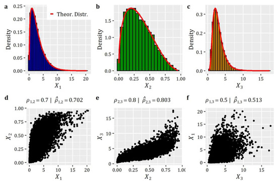
Figure 1.
Simulation of correlated RVs: (a–c) histograms of simulated data along with the target theoretical distribution functions; and (d–f) scatter plots depicting the established correlation between the 3 RVs under study.
We note that, using the same simulation method (and R-code already provided by anySim), it is possible to generate stationary and non-stationary non-Gaussian processes and fields [79], yet, in this work and in the following sections, we limit our focus on models (and code) particularly designed for the cases of stationary and cyclostationary processes as well as on stationary fields.
Box 2. R-code for the generation of correlated RVs with specific target marginal distributions and correlation matrix.
set.seed(13)
# Define the target distribution functions (ICDFs) of X1, X2 and X3 RV.
FX1=‘qgamma’; FX2=‘qbeta’; FX3=‘qlnorm’
Distr=c(FX1,FX2,FX3) # store the 3 ICDFs in a vector
# Define the parameters of the target distribution functions.
# and store them in a list
pFX1=list(shape=1.5,scale=2); pFX2=list(shape1=1.5,shape2=3)
pFX3=list(meanlog=1,sdlog=0.5)
DistrParams=list()
DistrParams[[1]]=pFX1;DistrParams[[2]]=pFX2;DistrParams[[3]]=pFX3
# Define the target correlation matrix.
CorrelMat=matrix(c(1,0.7,0.5,
0.7,1,0.8,
0.5,0.8,1),ncol=3,nrow=3,byrow=T);
# Estimate the parameters of the auxiliary Gaussian model.
paramsRVs=EstCorrRVs(R=CorrelMat,dist=Distr,params=DistrParams,
NatafIntMethod=‘GH’,NoEval=9,polydeg=8)
# Generate 10000 synthetic realisations of the 3 correlated RVs.
SynthRVs=SimCorrRVs(n=10000,paramsRVs=paramsRVs)
5.2. Simulation of Univariate Stationary Non-Gaussian Processes
Moving now to the use of anySim for the simulation of univariate stationary non-Gaussian processes, we demonstrate package capabilities via three distinct examples involving processes with continuous, discrete, and zero-inflated marginal distribution, respectively. The simulation scheme of this section is based to some extent on the so-called ARTA approach [76], with modifications regarding the order of the auxiliary Gp model, the use of theoretical ACS, and the method for the estimation of equivalent correlation coefficients. This scheme, termed as ARTA(p), is implemented via two key R-functions: the EstARTAp for the estimation of parameters of the auxiliary (Gaussian) AR(p) model and the SimARTAp for the generation of synthetic data according to a target stationary process. Further details on this modeling approach can be found in the literature [20,25,72,79], where the use alternative distribution models are discussed (e.g., three components mixtures, focusing also on the modeling of extremes), as well as high-order multivariate models are presented in detail [25,79].
Back to our case, the first example of the ARTA(p) scheme (see Box 3) concerns the simulation of a process with Gamma distribution (qgamma) and autocorrelation structure given by the product of a CAS (cscas) and a periodic ACS (csPeriodic). Particularly, we assume and .
In the second example (see Box 4), we assume that is a process with discrete distribution, specifically a Beta-Binomial (qbb), i.e., , and autocorrelation structure given by CAS (cscas), i.e., .
Finally, the third case (see Box 5) concerns the simulation of an intermittent process , described by a zero-inflated Generalized Gamma () marginal distribution (combination of qzi and qgengamma) with for the discrete part and for the continuous part. The process has an autocorrelation structure given by CAS (cscas), i.e., . We note that in this case the parameterization of the process resembles the empirical properties obtained from the hourly rainfall dataset of month July (extending over the period 1 September 1995 to 31 December 2017) at Oberstdorf, Germany (German Weather Service; station ID 3730) (for further details on this dataset and simulation cases, see also [25]).
The results of the three above-described simulation examples are summarized in Figure 2, where we can see the exact reproduction of the target distribution functions (including the probability of zero values for the case of second example—see Figure 2e) and the target autocorrelation structures.
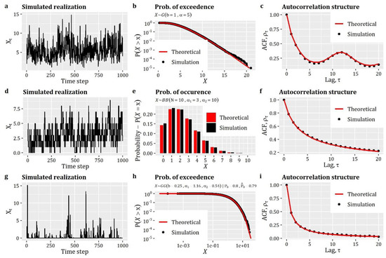
Figure 2.
Simulation of univariate stationary processes with: (first row, a–c) continuous distribution function; (second row, d–f) with discrete distribution; and (third row, g–i) with zero-inflated distribution. The figure displays: (first column, a, d and g) the simulated realization of the processes; (second column, b, e and h) the comparison between theoretical and simulated empirical probability plots; and (third column, c, f and i) the comparison between theoretical and simulated autocorrelation structures.
Box 3. R-code for the simulation of univariate stationary process with continuous marginal distribution and autocorrelation structure given by the product of a CAS and a periodic ACS.
set.seed(12)
# Define the target autocorrelation structure.
acsS=cscas(param=c(3,0.6),lag=1000) # CAS with b=3 and k=0.6
acsP=csPeriodic(param=c(12,1.5),lag=10^3) # Periodic with p=12 and l=1.5
ACS=acsP*acsS # The target ACS as product of the two previous ones
# Define the target distribution function (ICDF).
FX=‘qgamma’ # Gamma distribution
# Define the parameters of the target distribution.
pFX=list(shape=5,scale=1)
# Estimate the parameters of the auxiliary Gaussian AR(p) model.
ARTApar=EstARTAp(ACF=ACS,dist=FX,params=pFX,NatafIntMethod=‘GH’)
# Generate a synthetic series of 10000 length.
SynthARTAcont=SimARTAp(ARTApar=ARTApar,steps=10^4)
Box 4. R-code for the simulation of univariate stationary process with discrete marginal distribution and autocorrelation structure given by CAS.
set.seed(16)
# Define the target autocorrelation structure.
ACS=cscas(param=c(1.5,0.3),lag=1000) # CAS with b=1.5 and k=0.3
# Define the target distribution function (ICDF).
require(TailRank)
FX=‘qbb’ # the Beta-Binomial distribution
# Define the parameters of the target distribution.
pFX=list(N=10,u=3,v=10)
# Estimate the parameters of the auxiliary Gaussian AR(p) model.
ARTApar=EstARTAp(ACF=ACS,dist=FX,params=pFX,NatafIntMethod="MC")
# Generate a synthetic series of 10000 length.
SynthARTAdiscr=SimARTAp(ARTApar=ARTApar,steps=10^4)
Box 5. R-code for the simulation of univariate stationary process with zero-inflated marginal distribution and autocorrelation structure given by CAS.
set.seed(18)
# Define the target autocorrelation structure.
ACS=cscas(param=c(0.91,1.09),lag=1000) # CAS with b=0.91 and k=1.09
# Define the target distribution function (ICDF).
FX=‘qzi’ # Define that distribution is of zero-inflated type
# Define the distribution for the continuous part of the process.
# Here, a re-parameterized version of Gen. Gamma distribution is used.
qgengamma=function(p,scale,shape1,shape2){
require(VGAM)
X=qgengamma.stacy(p=p,scale=scale,k=(shape1/shape2),d=shape2)
return(X)
}
# Define the parameters of the zero-inflated distribution function.
pFX=list(Distr=qgengamma,p0=0.8,scale=0.25,shape1=1.16,shape2=0.54)
# Estimate the parameters of the auxiliary Gaussian AR(p) model.
ARTApar=EstARTAp(ACF=ACS,dist=FX,params=pFX,NatafIntMethod="GH",
NoEval=9,polydeg=8)
# Generate a synthetic series of 10000 length.
SynthARTAzi=SimARTAp(ARTApar=ARTApar,steps=10^4)
5.3. Simulation of Univariate Cyclostationary Non-Gaussian Processes
Further to stationary processes, anySim can also be used for the generation of univariate cyclostationary processes , reproducing the target lag-1 season-to-season correlations, as well as the seasonally varying target marginal distributions. Recall that a cyclostationary process consisted of sub-periods (e.g., months) can be denoted by or simply , where in that case the sub-period (i.e., season—e.g., month) that corresponds to a time step may be recovered by , while when . Moreover, the period (say ; e.g., year) may be obtained by .
For the simulation of univariate cyclostationary non-Gaussian processes, anySim implements the SPARTA model that is described in detail in the works of Tsoukalas et al. [21,25,77] (also used for monthly large-scale simulations of streamflow processes [142], as well as for the simulation of non-physical processes at hourly time scale; see Kossieris et al. [20]). The procedure is evolved via two key R-functions (see Box 6): the EstSPARTA function for the estimation of parameters of the auxiliary PAR(1) model and the SimSPARTA function for the generation of synthetic data according to a target cyclostationary process.
As a demo case, we examine the simulation of monthly runoff that is characterized by monthly seasonality, and hence it is treated as cyclostationary process with marginal distributions and correlation structures which vary periodically from month-to-month. We note that, in this case, the parameterization of the process resembles the empirical properties obtained from a monthly runoff series from Kremasta (Greece). Specifically, we aim to reproduce the fitted distributions of each month, which are either (qgengamma) or (qburr), as well as the empirical lag-1 season-to-season correlations (12 values).
Box 6 presents the R-code for the generation 10,000 data from the above defined cyclostationary process, while Figure 3 summarizes the results of the simulation. As can be seen, the method resembles the given season-to-season correlations (see Figure 3b), while the indicative empirical probability plots of Figure 3c,d demonstrate the efficiency of the method in terms of reproducing the target marginal behavior.
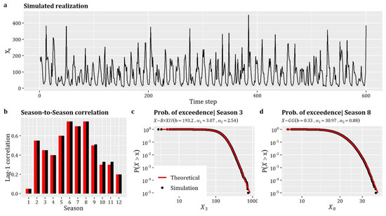
Figure 3.
Simulation of univariate cyclostationary processes: (a) simulated realization of the process; (b) comparison between theoretical and simulated Lag-1 season-to-season correlation coefficients; and (c,d) comparison between theoretical and simulated empirical probability plots.
Box 6. R-code for the simulation of univariate cyclostationary process with specific distribution function at each season and specific lag-1 season-to-season correlations.
set.seed(21)
# Define the number of seasons.
NumOfSeasons=12 # number of months
# Define the (12) lag-1 season-to-season correlation coefficients
rtarget<-c(0.05,0.55,0.45,0.4,0.6,0.75,0.7,0.75,0.5,0.3,0.3,0.2)
# Define the target distribution functions for each season.
# In this example, the Gen. Gamma distribution is used in the
# formulation given in Box 5.
# Or, a re-parameterized version of Burr type-XII distribution.
qburr=function(p,scale,shape1,shape2) {
require(ExtDist)
x=ExtDist::qBurr(p=p,b=scale,g=shape1,s=shape2)
return(x)
}
# Here, we define the target distribution of each season as a zero-
# inflated, though being of continuous type, to demonstrate the more
# general case. Alternatively, the definition can be conducted as in
# EstARTAp function (see Box 2).
# Define that distributions are of zero-inflated type.
FXs<-rep(‘qzi’,NumOfSeasons)
# Define the parameters of the distribution function for each season.
PFXs<-vector("list",NumOfSeasons)
PFXs[[1]]=list(p0=0.0,Distr=qgengamma,scale=47.22,shape1=2.7,shape2=0.97)
PFXs[[2]]=list(p0=0.0,Distr=qgengamma,scale=199.4,shape1=1.74,shape2=3.45)
PFXs[[3]]=list(p0=0.0,Distr=qburr,scale=193.2,shape1=3.07,shape2=2.54)
PFXs[[4]]=list(p0=0.0,Distr=qburr,scale=172.16,shape1=4.42,shape2=2.50)
PFXs[[5]]=list(p0=0.0,Distr=qgengamma,scale=53.40,shape1=4.11,shape2=1.66)
PFXs[[6]]=list(p0=0.0,Distr=qgengamma,scale=0.017,shape1=26.23,shape2=0.51)
PFXs[[7]]=list(p0=0.0,Distr=qgengamma,scale=27.70,shape1=5.15,shape2=5.30)
PFXs[[8]]=list(p0=0.0,Distr=qgengamma,scale=0.33,shape1=30.97,shape2=0.876)
PFXs[[9]]=list(p0=0.0,Distr=qburr,scale=14.46,shape1=7.6,shape2=0.44)
PFXs[[10]]=list(p0=0.0,Distr=qburr,scale=29.36,shape1=2.73,shape2=0.87)
PFXs[[11]]=list(p0=0.0,Distr=qgengamma,scale=53.15,shape1=3.12,shape2=1.4)
PFXs[[12]]=list(p0=0.0,Distr=qgengamma,scale=116.02,shape1=2.21,shape2=1.3)
# Estimate the parameters of SPARTA model.
SPARTApar<-EstSPARTA(s2srtarget=rtarget, dist=FXs, params=PFXs,
NatafIntMethod=‘GH’, NoEval=9, polydeg=8, nodes=11)
# Generate a cyclostationary synthetic series of 10000 length.
simSPARTA<-SimSPARTA(SPARTApar=SPARTApar, steps=10^4)
5.4. Simulation of Multivariate Stationary Processes with Continuous and Zero-Inflated Marginal Distributions
This section focuses on the case of multivariate stationary processes and demonstrates the functionalities of anySim through a simulation example involving three contemporaneously cross-correlated processes, i.e., . In this case, apart from auto-dependence, the processes exhibit cross-dependence at lag-0. It is noted that such type of simulation may regard different processes at the same location (e.g., humidity, rainfall, and temperature) or processes of the same type (e.g., rainfall) at different locations. In this simulation study, we focus on the former case, assuming that the three processes represent the daily humidity, rainfall, and temperature, respectively, of a specific month (to support the assumption of stationarity).
For the simulation of multivariate stationary processes, anySim implements the SMARTA(q) model [78] via two key R-functions (see Box 7): the EstSMARTA function for the estimation of parameters of the auxiliary (Gaussian) SMA model and the SimSMARTA function for the generation of synthetic data.
In this simulation example, we assume a Beta distribution (qbeta) for humidity (i.e., ), a zero-inflated Generalized Gamma distribution (; combination of qzi and qgengamma) for rainfall (i.e., ), and a Normal distribution (qnorm) for temperature (i.e., ). Regarding the auto-dependence structure, we employed the CAS (cscas) with different parameters for each process, i.e.,, and , where . Finally, the three processes were assumed contemporaneously cross-correlated, as given by the following lag-0 cross-correlation matrix (parameter Cmat in EstSMARTA), where each element represents the lag-0 correlation, . Specifically, the target matrix is given by:
Note that the parameters of the marginal distributions, as well as those of the ACSs and lag-0 correlations, were not obtained from observed data but they were chosen to realistically represent the hypothesized processes.
Box 7 presents the R-code for the generation of a 3-dimensional realization with 214 time steps according to the above simulation scenario, while the results of this example are summarized graphically in Figure 4. As can be seen, the method enables the reproduction of the target distribution function and autocorrelation structure of all three processes (see Figure 4d–i), while the scatter plots in Figure 4j–l provide an illustrative representation of the established cross-dependencies among the processes. Figure 4j–l also highlights the efficiency of the method in terms of reproducing the lag-0 cross-correlation coefficients (as shown in the titles of Figure 4j–l where the target and simulated lag-0 cross-correlation coefficients are presented).
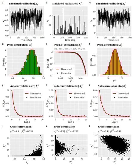
Figure 4.
Simulation of multivariate stationary processes: (a–c) simulated realizations of the three correlated processes (randomly selected window of 1000 time steps); (d–e) comparison between theoretical and simulated empirical probability plots; (g–i) comparison between theoretical and simulated autocorrelation structures; and (j–l) scatter plots depicting the lag-0 cross-correlation between the 3 processes under study.
Box 7. R-code for the simulation of multivariate stationary processes with specific distribution functions and autocorrelation structures, as well as specific lag-0 cross-correlation matrix.
set.seed(9)
# Define the target autocorrelation structure of the 3 processes.
ACSs=list()
ACSs[[1]]=cscas(param=c(0.1,0.7),lag=2^6)
ACSs[[2]]=cscas(param=c(0.2,1),lag=2^6)
ACSs[[3]]=cscas(param=c(0.1,0.5),lag=2^6)
# Define the matrix of lag-0 cross-correlation coefficients.
Cmat=matrix(c(1,0.4,-0.5,
0.4,1,-0.3,
-0.5,-0.3,1),ncol=3,nrow=3)
# Define the target distribution functions (ICDF) of the 3 processes
# Define that distributions are of zero-inflated type.
FXs=rep(‘qzi’,3)
# Define the distributions for the continuous part of the processes.
# In this example, the Gen. Gamma distribution is used in the
# formulation given in Box 5.
# Define the parameters of the target distributions.
pFXs[[1]]=list(Distr=qbeta,p0=0,shape1=15,shape2=5) # Beta distribution
pFXs[[2]]=list(Distr=qgengamma,p0=0.7,scale=0.12, shape1=1.35, shape2=0.4) # Gen. Gamma
pFXs[[3]]=list(Distr=qnorm,p0=0,mean=15,sd=3) # Normal distribution
# Estimate the parameters of SMARTA model
SMAparam=EstSMARTA(dist=FXs,params=pFXs,ACFs=ACSs,Cmat=Cmat,
DecoMethod=‘cor.smooth’,FFTLag = 2^7,
NatafIntMethod=‘GH’,NoEval=9,polydeg=8)
# Generate the synthetic series of 2^14 length.
simSMARTA=SimSMARTA(SMARTApar=SMAparam,steps=2^14,SMALAG=2^6)
5.5. Simulation of Spatiotemporal Random Fields with Zero-Inflated Marginal Distributions
Beyond stochastic processes, anySim can also be used for simulation of spatiotemporal random fields (RFs). Particularly, the currently implemented model in anySim model called SMARTA(q), is able to simulate homogenous and stationary non-Gaussian RFs, and to generate realizations reproducing the field’s target marginal distribution, temporal correlation structure (up to time lag equal to q) and lag-0 spatial correlation structure. The simulation is performed using two functions of the package: EstSMARTA_RFs (a faster version of EstSMARTA function, designed for RFs) and SimSMARTA.
To provide a bit more context, let be a spatiotemporal RF, where in this case the index refers to a spatial position in and the index refers to time. Further to this, assuming a discretized RF in × grid consisting of total points, allows us to view the RF as a -dimensional multivariate process, that is, , where each process at point is associated with coordinates , where denote the horizontal and vertical coordinates respectively. Let us also assume that the RF is characterized by a marginal distribution with finite variance, while stand for the spatiotemporal correlation structure of the RF (which is assumed to be positive definite) which depends on the spatial (Euclidean) distance of two points and , and the time lag .
To simulate a RF with anySim, the first step is to discretize it through the definition of a × grid (where and stand for the number of cells in the horizontal and vertical direction, respectively). Such an example is given in Figure 5, where a field is discretized with 5 × 5 grid points, where each point represents the center of the cell (see also Lines 1–7 in Box 8). Having done that, it is straightforward to see what is mentioned above, i.e., that the simulation of a spatiotemporal RF can be viewed as a multivariate simulation problem of × processes. Hence, we may employ the multivariate SMARTA(q), or any other multivariate (Nataf-based) ARMA-type model (see, for instance, Appendix B in Tsoukalas et al. [25] and Section 5.4 in Tsoukalas [79], who elaborated on high-order AR Nataf-based models, as well as Papalexiou and Serinaldi [73], who employed high-order AR models for the simulation of RFs), to simulate the spatiotemporal RF. Moving to the re-formulated RF simulation problem, i.e., to simulate a multivariate process , it is recalled that represents the process at cell , which, in this case, due to properties of homogeneity and stationarity, all cells have the same marginal distribution and ACS (hence, it is straightforward to parameterize accordingly the SMARTA(q) model), while their CCS is solely determined by the distance among the points. In particular, for each , we have the corresponding coordinates , hence we can easily compute, e.g., the Euclidean, distance among any two points and via . Having done that, and using the target theoretical spatiotemporal correlation structure, we can now specify the required (by SMARTA(q) model) lag-0 cross-correlation coefficients among the × processes (parameter Cmat in EstSMARTA_RFs).
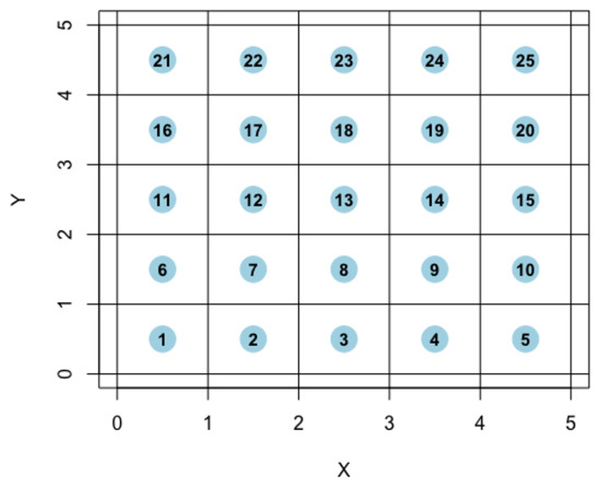
Figure 5.
Discretization of a random field with 5 × 5 grid points.
The simulation example presented here (Box 8) regards the simulation of a homogenous, stationary, and isotropic spatiotemporal RF with marginal and correlation properties that mimic those of an intermittent rainfall field.
Particularly, regarding the RF’s properties and the parameterization of EstSMARTA, it was assumed that the marginal distribution of the RF was identical to the one fitted to the daily rainfall data recorded at Bologna, Italy gauge. Since the RF is an intermittent one, we employed a zero-inflated Burr Type-XII distribution () [143,144] marginal distribution, denoted by (combination of qzi and qburr) with for the discrete part and for the continuous part.
Further to this, to model the spatiotemporal CS of the RF, we employed a separable (product) model, where both the ACS and CCS are given by CAS (cscas). Particularly, the former is given by, while the latter is given by . Therefore, the spatiotemporal CS can be expressed as the product of these two CS, i.e., .
Moving to the simulation results, Figure 6 illustrates 30 snapshots (depicting the evolution of the RF among consecutive time steps) of a RF simulated using the aforementioned characteristics in grid over ~30,000 time steps (which, assuming a daily time step, corresponds to about 82 years of synthetic data). Additionally, Figure 7 provides a comparison among the target and simulated RF in terms of reproducing: (a) the target distribution; (b) the target autocorrelation structure; and (c) the target lag-0 cross-correlation structure. In a similar vein, Figure 8 compares some key statistics among the target and simulated RF. Particularly, it depicts for each cell: (a) the probability dry; (b) the mean; (c) the L-scale; and (d) the L-skewness. Arguably, the good agreement between target and simulated properties, depicted in Figure 7 and Figure 8, highlight the ability of the model to simulate RFs with the target properties with high accuracy.
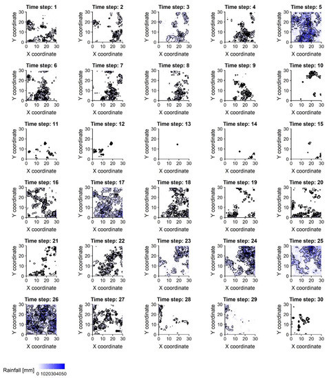
Figure 6.
Time step (1–30) of the simulated non-Gaussian spatiotemporal RF, spanning across 30 time steps. White cells represent cells with zero values (i.e., no rainfall), while blue color palette is used to depict the non-zero values (light rainfall is depicted with light blue, while heavy rainfall with dark blue).
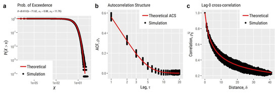
Figure 7.
Comparison between RF’s target and simulated: (a) distribution function; (b) autocorrelation structure; and (c) lag-0 cross-correlation.
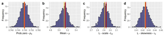
Figure 8.
Comparison between RF’s target and simulated key statistics, particularly: (a) probability dry; (b) mean; (c) L-scale; and (d) L-skewness.
Box 8. R-code for the simulation of a spatiotemporal random field (RF) with specific distribution function, autocorrelation structure (temporal), as well as specific lag-0 cross-correlation structure (spatial).
# Define a 30x30 grid to be simulated.
nx=30 # number of cells in the horizontal direction
ny=30 # number of cells in the vertical direction
Sites=nx*ny # number of grid points
Xp=seq(from=(0.5),to=nx,by=1) # points’ coordinates in horizontal axis
Yp=seq(from=(0.5),to=ny,by=1) # points’ coordinates in vertical axis
grid=expand.grid(X=Xp,Y=Yp)
# Estimate the Euclidean distances between grid points.
DZ=dist(x=grid,method=‘euclidean’,upper=T,diag=T)
DZmat=as.matrix(DZ)
EuclDist=DZmat[upper.tri(DZmat, diag = T)]
# Define the matrix of lag-0 cross-correlations among grid points.
CCF=(1+0.2*2*EuclDist)^(-1/b) # CAS with b=0.2 and k=2.
Cmat=matrix(NA,nrow=nx*ny,ncol=nx*ny)
Cmat[upper.tri(Cmat,diag=T)]=CCF
Cmat[lower.tri(Cmat,diag=T)]=rev(CCF)
# Define the target autocorrelation structure and
# distribution function (ICDF) at each point.
# The distribution functions are of zero-inflated type.
# For the continuous part, the Burr type-XII distribution is used
# in the formulation given in Box 6.
FXs=rep(‘qzi’,Sites) # Define that distributions are zero-inflated.
PFXs=vector("list",length=Sites) # List with ICDF of each point
ACFs=vector("list",length=Sites) # List with ACF of each point
for (i in 1:Sites) {
PFXs[[i]]=list(Distr=qburr,p0=0.75,scale=71.62,shape1=0.88,shape2=11.79)
ACFs[[i]]=cscas(param=c(0.1,0.6),lag=2^6) # CAS with b=0.1 and k=0.6
}
# Estimate the parameters of SMARTA model
SMAparam=EstSMARTA_RFs(dist=FXs,params=PFXs,ACFs=ACFs,Cmat=Cmat,
DecoMethod=‘cor.smooth’,FFTLag=2^7,
NatafIntMethod=‘GH’,NoEval=9,polydeg=8)
# Generate a synthetic realisation of random fields with 2^15 length
SimField=SimSMARTA(SMARTApar=SMAparam,steps=2^15,SMALAG=2^6)
5.6. Univariate Disaggregation of Coarser-Level Stationary Series to Finer-Level Stationary Series
The cases examined so far concern the stochastic simulation of processes and fields at a single temporal scale. This simulation study, as well as the following one, focuses on the multi-scale simulation of stochastic processes, which targets the reproduction of the marginal and stochastic properties of a process at multiple temporal scales. As discussed in Section 2.4, this problem holds a prominent position in the modeling of hydrometeorological processes and anySim addresses it by implementing functions that support disaggregation, i.e., generation of synthetic time series at a lower temporal scale which sum up exactly to the given coarser-level data.
Here, we study the problem of disaggregating daily rainfall from a single station into 10-min amounts. The disaggregation scheme is applied to a 10-min rainfall dataset from Soltau, Germany (Station ID 4745), extending from 1999 to 2009 with 0.24% missing values. To cope with the effect of seasonality, we assume that the rainfall process within each monthly period is stationary (i.e., cyclical stationarity from month-to-month). To save space, the R-code presented in Box 9 and the results in Figure 9 and Figure 10 concern only the case of January, while the computational procedure is identical for the other months (i.e., by seasonally varying the model’s parameters).
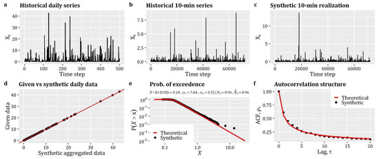
Figure 9.
Historical (a) daily and (b) 10-min rainfall series; (c) synthetic (disaggregated) 10-min rainfall realization; (d) consistency check, comparing the values of the aggregated synthetically generated 10-min data, i.e., when aggregated to daily scale, with the corresponding target values; (e) comparison of distribution function of non-zero amounts for 10-min historical and disaggregated series (the fitted theoretical model is shown with red line); and (f) comparison of autocorrelation function (ACF) for 10-min historical and disaggregated series (the fitted theoretical model is shown with the red line).
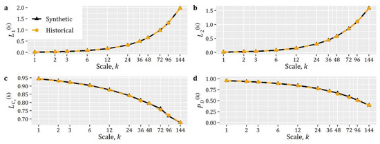
Figure 10.
Comparison of historical (empirical) and synthetically (disaggregated) generated data, as a function of aggregation scale , in terms of: (a) L-mean (); (b) L-scale (); (c) L-skewness (); and (d) probability dry ().
anySim implements the NDA approach (see Tsoukalas et al. [25], as well as Section 2.4) via Disagg_ARTAp R-function that enables the disaggregation of a stationary coarser-level series to a stationary one at a finer level. The key input arguments of this R-function are the higher-level series (input argument HLSeries) and the parameters of ARTA(p) model (input argument ARTApar) that control the lower-level stationary model (see Section 3.2).
For the simulation of the lower-level (10-min) process, we assume a Burr Type-XII (qburr) distribution, i.e., , and an autocorrelation structure, given by CAS (cscas; see Section 2.5), which has been fitted to the empirical estimates of autocorrelation coefficients up to time lag 24, i.e., . The parameters of the auxiliary (Gaussian) AR(p) model are estimated via EstARTAp function.
Here, instead of disaggregating the observed daily rainfall amounts, we choose to disaggregate a synthetic daily series to demonstrate a more general case where the series at both temporal scales are product of simulation models. To keep things simple (and not use an additional simulation model for the daily scale), we employ the above fitted ARTA(p) model to generate a realization of 10-min values that are summed up to compose the daily values that are then disaggregated. It is also noted that in this case the associated R-function requires about 390 s to disaggregate 500 daily values to 10-min sequences (by setting the parameter max.iter = 500 in Disagg_ARTAp).
The results of this simulation example are presented in Figure 9 and Figure 10. As shown in Figure 9d, the procedure establishes full consistency between the synthetic 10-min data (when aggregated to daily scale) and the corresponding target values. Additionally, the empirical probability distribution of disaggregated data resembles the target one (see Figure 9e), while the same also stands for the autocorrelation structure (see Figure 9f). For an additional validation, we also estimate several statistical quantities (that is, probability zero and the first three L-moments) across multiple scales, i.e., , where stands for the 10-min time scale (e.g., and refer to 20-min and daily temporal scale, respectively). Figure 10 shows that the disaggregation procedure enables the reproduction of the above statistical quantities also at the intermediate temporal scales, further to 10-min and daily scale.
Box 9. R-code for the generation of synthetic univariate stationary series at a higher level and its disaggregation into finer-level cyclostationary series.
set.seed(124)
# Define the target autocorrelation structure of finer-level process.
ACS=cscas(param=c(1.688,1), lag=24) # CAS with b=1.688 and k=1
# Define the target distribution function (ICDF).
FX=‘qzi’ # Define that distribution is of zero-inflated type
# Define the distribution for the continuous part of the process.
# In this example, the Burr type-XII distribution is used in the
# formulation given in Box 6.
# Define the parameters of the zero-inflated distribution function.
pFX=list(p0=0.96,Distr=qburr,scale=0.181,shape1=7.642,shape2=0.296)
# Estimate the parameters of the auxiliary Gaussian AR(p) model.
param=EstARTAp(ACF=ACS,dist=FX, params=pFX, NatafIntMethod=‘GH’)
# Compose the daily series to be disaggregated
Sim=SimARTAp(ARTApar=param, burn=1000, steps=(24*6*500))
DailySeries=apply(X=matrix(data=Sim$X, ncol=24*6,byrow=1),MARGIN=1,FUN=sum)
## Disaggregate the daily series to 10-min data
disag10min=Disagg_ARTAp(HLSeries=DailySeries,ARTApar=param,
max.iter=500,steps=24*6)
5.7. Univariate Disaggregation of Coarser-Level Stationary Series to Finer-Level Cyclostationary Series
This simulation study concerns the synthesis of multi-scale consistent monthly streamflow data (1000 years; Figure 11b), based on the widely-known dataset of Nile River at Aswan dam ([145]; Figure 11a). As discussed previously, the reproduction of the marginal and correlation properties of a process at a single temporal level does not ensure the preservation of the characteristics of the process at the higher aggregation levels. In this vein, the SPARTA model can be employed to generate stochastically consistent synthetic monthly series at monthly scale (see simulation example in Section 5.3), but the annual properties (and especially the LRD behavior) of the Nile streamflow data will not be reproduced. Having said this, the objective of this simulation case is to generate a synthetic realization of a cyclostationary process at monthly scale (the basic one, denoted by ) with the desired marginal distributions and season-to-season correlations, which when aggregated to the annual scale (i.e., ), i.e., (where is the time index of the aggregated process) will result in a realization of the annual process which exhibits the target annual marginal distribution and autocorrelation structure.
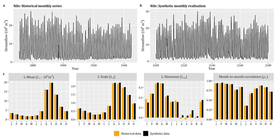
Figure 11.
(a) Historical Nile monthly streamflow series (March 1870 to December 1945); and (b) synthetically generated time series using the anySim package (randomly selected window of 80 years). Monthly-based comparison of historical and simulated (bottom row (c)) L-mean, L-scale, and L-skewness, as well as lag-1 month-to-month correlations coefficients.
To accomplish the above objective, anySim implements the so-called NDA approach [25] via Disagg_SPARTA R-function that enables the disaggregation of a stationary coarser-level series to a finer cyclostationary one. The key input arguments of this R-function are the higher-level series (input argument HLSeries) and the parameters of SPARTA model (input argument SPARTApar) that control the lower-level cyclostationary model (see Section 3.2).
As in the previous simulation example, to demonstrate a more general case (see Box 10), we use the ARTA(p) scheme (SimARTAp; see Section 5.2) to generate a stationary synthetic series at the coarser-level (annual), which resemble the marginal and stochastic characteristics of the observed annual streamflow of Nile. For the simulation of the annual process, we assume a Generalized Gamma (qgengamma) distribution, i.e., , and an autocorrelation structure given by CAS (cscas; see Section 2.5), which has been fitted to the empirical estimates of autocorrelation coefficients up to time lag 10, i.e., . The parameters of the auxiliary (Gaussian) AR(p) model are estimated via EstARTAp function. Regarding the parameterization of the cyclostationary process at the lower temporal level (monthly), we fit either a Generalized Gamma (qgengamma) or a Burr Type-XII (qburr) distribution to each month, as well as estimate the empirical lag-1 month-to-month correlations (12 values) of the Nile streamflow data.
The results of this simulation example are presented in Figure 12, Figure 13 and Figure 14. Starting from the simulation of the higher-level process, Figure 12 reveals the ability of ARTA(p) scheme to reproduce the target marginal and stochastic properties of annual Nile streamflow. Moving to the finer scale, as shown in Figure 13, the empirical probability distributions of the disaggregated data at monthly scale resemble the target theoretical distributions for all 12 months. Finally, Figure 14 shows that the empirical lag-1 month-to-month correlations are well reproduced without sacrificing realism in the established dependence patterns (see also the relevant discussion by Tsoukalas et al. [22]).
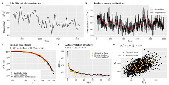
Figure 12.
(a) Historical annual time series of Nile streamflow at Aswan Dam; (b) synthetic time series (1000 years); (c) empirical, simulated, and theoretical distribution function, with the parameters of the theoretical distribution given in the title of the plot; (d) empirical, simulated, and theoretical and autocorrelation coefficients, with the parameters of CAS given in the title of the plot; and (e) scatter plot of annual historical and synthetic time series for time lag 1.
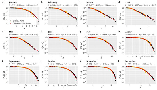
Figure 13.
Monthly-based (a–l) comparison of empirical, simulated, and theoretical distribution functions. The title of each subplot provides the selected distribution and its parameters.
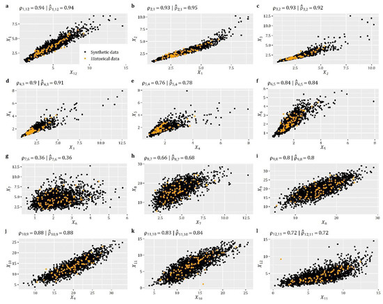
Figure 14.
Month-to-month (a–l) scatter plots of historical and simulated Nile streamflow data (109 m3). The title of each subplot provides the lag-1 month-to-month target and simulated correlation coefficients.
Box 10. R-code for the generation of synthetic univariate stationary series at a higher level and its disaggregation into finer-level cyclostationary series.
## Simulation of coarser-level (Annual) stationary process ##
# Define the target autocorrelation structure of coarser-level process
ACS_annual=cscas(param=c(2.623,1.557),lag=200)
# Define the target distribution function of coarser-level process.
# In this case, the Gen. Gamma distribution is used in the
# formulation given in Box 5.
FX=‘qgengamma’
# Define the parameters of the target distribution.
pFX=list(scale=7.419,shape1=20.493,shape2=1.198)
# Estimate the parameters of the auxiliary Gaussian AR(p) model.
ARTApar=EstARTAp(ACF=ACS_annual,dist=FX,params=pFX,NatafIntMethod=‘GH’)
# Generate the annual synthetic series of 10000 length.
simAnnual=SimARTAp(ARTApar = ARTApar, steps = 10^3)
## Simulation of lower-level (Monthly) cyclostationary process ##
# Define the number of seasons.
NumOfSeasons=12 # number of months
# Define the lag-1 season-to-season correlation coefficients
# (12 values) of monthly Nile Streamflow.
rtarget_mon=c(0.938,0.931,0.926,0.903,0.761,0.837,0.355,0.662,0.796,0.876,0.826,0.720)
# Define the target distribution functions for each season.
# In this example, the Gen. Gamma or Burr type-XII distribution are
# used in the formulations given in Box 5 and 6, respectively
FXs=c(‘qgengamma’,‘qburr’,‘qburr’,‘qburr’,‘qburr’,‘qgengamma’,‘qgengamma’,‘qgengamma’,‘qgengamma’,‘qgengamma’,‘qgengamma’,‘qgengamma’)
# Define the parameters of distribution functions for each season.
PFXs<-vector("list",NumOfSeasons)
PFXs[[1]]=list(scale=0.000862254,shape1=18.24168,shape2=0.4491688)
PFXs[[2]]=list(scale=2.352517,shape1=6.233872,shape2=0.7284742)
PFXs[[3]]=list(scale=1.586728,shape1=9.007934,shape2=0.4096283)
PFXs[[4]]=list(scale=1.337449,shape1=12.01606,shape2=0.3374601)
PFXs[[5]]=list(scale=1.56249,shape1=6.386645,shape2=0.8020387)
PFXs[[6]]=list(scale=0.0005479373,shape1=18.54147,shape2=0.4500553)
PFXs[[7]]=list(scale=0.001297873,shape1=19.83979,shape2=0.4629369)
PFXs[[8]]=list(scale=15.27454,shape1=5.607777,shape2=3.654064)
PFXs[[9]]=list(scale=17.18964,shape1=7.913649,shape2=3.848175)
PFXs[[10]]=list(scale=8.327586,shape1=7.307034,shape2=2.280058)
PFXs[[11]]=list(scale=9.226506,shape1=2.42338,shape2=4.200226)
PFXs[[12]]=list(scale=0.002727125,shape1=14.18116,shape2=0.4648454)
# Estimate the parameters of SPARTA model.
SPARTApar<-EstSPARTA(s2srtarget=rtarget_mon,dist=FXs,params=PFXs,
NatafIntMethod=‘GH’,NoEval=9,polydeg=8,nodes=11)
# Disaggregate the annual series to monthly amounts.
disagMonthly<-Disagg_SPARTA(HLSeries=simAnnual$X[1:100], SPARTApar=SPARTApar,max.iter=300,steps=NumOfSeasons)
6. Conclusions
In an attempt to fill the gap of limited availability of general and open-source software for stochastic modeling purposes, this work introduces and details a freely available R-package, called anySim. The package implements a suite of state-of-the art models, all based on the notion of Nataf’ joint distribution model (i.e., Gaussian copula), which facilitate the simulation of non-Gaussian correlated random variables, stochastic processes, and random fields. anySim covers the needs of these three omnipresent modeling tasks, and aims this way to provide an easy-to-use, one-stop solution for practitioners, engineers, and researchers working towards the development of a variety of uncertainty-related applications (e.g., development of Monte-Carlo-type experiments for engineering and environmental studies).
More specifically, as demonstrated through several simulation examples, focusing mostly on hydrometeorological processes (i.e., generation of synthetic weather data, such as rainfall, streamflow, and temperature), the current version of anySim is able to perform tasks that regard:
- The simulation of non-Gaussian correlated random variables with target correlation matrix.
- The simulation of non-Gaussian univariate and multivariate processes with given target auto-correlation and lag-0 cross-correlation structure.
- The simulation of non-Gaussian univariate processes (stationary and cyclostationary) at multiple temporal scales, preserving the target distributions, as well as the target auto-correlation structures at multiple temporal scales.
- The disaggregation of univariate coarser-level sequences to finer-level sequences exhibiting the target (non-Gaussian) distributions and auto-correlation structure.
- The simulation of non-Gaussian homogenous random fields with target spatiotemporal correlation structure (preserving the lag-0 contemporaneous spatial correlations, as well as autocorrelation up to large time lags).
Beyond these, anySim offers a scale-free approach since the implemented simulation models are suitable for processes/fields of any time (or spatial) scale and can be used as long as the models are being parameterized by any marginal distribution (including zero-inflated models; to account for processes/fields characterized by intermittency, such as rainfall) with finite variance and valid correlation structure (i.e., positive definite). It is remarked that in the cases where the last constraint is not satisfied, anySim can still be employed if combined with procedures that correct non-positive definite matrices [34,146], i.e., identify a valid (nearest) correlation structure in case of inconsistency. However, this problem is not encountered throughout the simulation studies presented herein.
Going beyond the current version of anySim, the package is viewed as dynamic entity that will be continuously enhanced with new functionalities. Ongoing research in this direction includes:
- The implementation of alternative multivariate models (for stationary and cyclostationary processes) for both simulation and disaggregation purposes.
- The implementation of methods and functions for conditional simulations.
- The implementation of alternative correlation structures (i.e., spatial, temporal, or combination of them), as well as methods that correct potential non-positive definite correlation structures.
- The implementation of functions dedicated for fitting distribution functions and correlation structures to historical data.
- Introduction of stochastic methods that rely on alternative copulas [138,139], such as asymmetric ones (e.g., Clayton and Gumbel copulas). This way, beyond NDM-based methods (i.e., Gaussian copula), which are suitable for symmetric dependence structures, anySim could be employed to describe more complex dependencies and thus further extend the simulation capabilities of the package (e.g., reproduction of extremes; tail dependencies).
- The implementation of some part of the code, and especially the more time-consuming functions (e.g., those related with disaggregation), in other programming languages (e.g., C++) to speed-up the package’s run times.
To conclude, it is argued that anySim brings into fruition, as well as practical implementation in real-world studies, the desideratum of Klemeš and Borůvka [86], highlighted by Tsoukalas et al. [21], for generalized generation schemes which are able to represent processes from any distribution and any correlation structure, thus moving beyond the classical paradigm of stochastic modeling in hydrology that aim at the resemblance of a process/field in terms of summary statistical characteristics and low-order correlations (cf. [147]). Of course, the need and utility of non-Gaussian models spans beyond the realm of hydrology and engineering, since it is widely acknowledged that such processes are omnipresent in many other scientific domains, such as, finance, biology, communication networks, and operations research. It is our belief, and hope, that anySim can and may find fertile ground of application also in such domains, and hopefully resolve existing problems and trigger new developments.
Author Contributions
I.T. and P.K. conceived and designed the present study, as well as developed the R code of anySim package. I.T. and P.K. designed and run the simulation examples presented herein, as well as developed the R code for the associated visualizations. I.T., and P.K. organized, prepared and drafted the manuscript. Funding acquisition by I.T. C.M. supervised the work during all stages. All authors have read and agreed to the published version of the manuscript.
Funding
This research is co-financed by Greece and the European Union (European Social Fund- ESF) through the Operational Programme “Human Resources Development, Education and Lifelong Learning“ in the context of the project “Reinforcement of Postdoctoral Researchers—2nd Cycle” (MIS-5033021), implemented by the State Scholarships Foundation (ΙΚΥ).

Acknowledgments
Data availability: The 1 h and 10 min rainfall data, mentioned in Section 5.2 and Section 5.6, respectively, are provided by the German Weather Service (Deutscher Wetterdienst; DWD) and are accessible via: https://www.dwd.de/EN/climate_environment/cdc/cdc.html. The historical dataset of runoff of Achelous river basin upstream of Kremasta dam in Western Greece (employed in Section 5.3) is available at: www.itia.ntua.gr/1914/. The historical dataset of daily rainfall at the gauging station of Bologna, Italy (used in Section 5.5) can be found at the Global Historical Climatology Network—Daily (GHCN-D) dataset, accessible from KNMI Climate Explorer (http://climexp.knmi.nl/). The Nile streamflow data at Aswan dam (see Section 5.7) can be retrieved from an external source (http://www.stats.uwo.ca/faculty/mcleod/epubs/mhsets/). Code availability: The source code of anySim R package is available GitHub repository at: https://github.com/itsoukal/anySim.
Conflicts of Interest
The authors declare no conflict of interest.
Appendix A. Distribution Functions Used to Demonstrate anySim
The probability density function (PDF) of the Gamma distribution () is given by,
where and are shape and scale parameters, respectively, while stands for the gamma function.
The probability density function (PDF) of the Beta distribution () is given by,
where are shape parameters, while .
The PDF of the three-parameter log-Normal distribution () is given by,
where ,, and denote the shape, scale. and location parameters. respectively. When the model reduces to its classical two-parameter variant.
The PDF of the Generalized Gamma () distribution is given by [148],
where denotes the gamma function, while and are shape parameters and is a scale parameter.
The PDF of the Burr Type-XII distribution () is [143,144],
where are shape parameters and is a scale parameter. It is noted that the rth moment of the distribution is finite, if and only if, .
The probability mass function (PMF) of the Beta-Binomial distribution () is given by,
where is a parameter denoting the number of trials (a positive integer) and and are both shape parameters.
References
- Kisiel, C.C. Transformation of deterministic and stochastic processes in hydrology. In Proceedings of the International Symposium in Hydrology, Fort Collins, CO, USA, 11–14 September 1967; Volume 1, pp. 600–607. [Google Scholar]
- Klemeš, V. Water storage: Source of inspiration and desperation. In Reflections on Hydrology: Science and Practice; American Geophysical Union: Washington, DC, USA, 1997; ISBN 9781118668085. [Google Scholar]
- Koutsoyiannis, D.; Economou, A. Evaluation of the parameterization-simulation-optimization approach for the control of reservoir systems. Water Resour. Res. 2003, 39. [Google Scholar] [CrossRef]
- Celeste, A.B.; Billib, M. Evaluation of stochastic reservoir operation optimization models. Adv. Water Resour. 2009, 32, 1429–1443. [Google Scholar] [CrossRef]
- Haberlandt, U.; Hundecha, Y.; Pahlow, M.; Schumann, A.H. Rainfall generators for application in flood studies. In Flood Risk Assessment and Management; Springer: Berlin/Heidelberg, Germany, 2011; pp. 117–147. [Google Scholar]
- Giuliani, M.; Herman, J.D.; Castelletti, A.; Reed, P. Many-objective reservoir policy identification and refinement to reduce policy inertia and myopia in water management. Water Resour. Res. 2014, 50, 3355–3377. [Google Scholar] [CrossRef]
- Tsoukalas, I.; Makropoulos, C. A Surrogate Based Optimization Approach for the Development of Uncertainty-Aware Reservoir Operational Rules: the Case of Nestos Hydrosystem. Water Resour. Manag. 2015, 29, 4719–4734. [Google Scholar] [CrossRef]
- Tsoukalas, I.; Makropoulos, C. Multiobjective optimisation on a budget: Exploring surrogate modelling for robust multi-reservoir rules generation under hydrological uncertainty. Environ. Model. Softw. 2015, 69, 396–413. [Google Scholar] [CrossRef]
- Tsoukalas, I.; Kossieris, P.; Efstratiadis, A.; Makropoulos, C. Surrogate-enhanced evolutionary annealing simplex algorithm for effective and efficient optimization of water resources problems on a budget. Environ. Model. Softw. 2016, 77, 122–142. [Google Scholar] [CrossRef]
- Feng, M.; Liu, P.; Guo, S.; Gui, Z.; Zhang, X.; Zhang, W.; Xiong, L. Identifying changing patterns of reservoir operating rules under various inflow alteration scenarios. Adv. Water Resour. 2017, 104, 23–36. [Google Scholar] [CrossRef]
- Do, N.C.; Razavi, S. Correlation Effects? A Major but Often Neglected Component in Sensitivity and Uncertainty Analysis. Water Resour. Res. 2020, 56. [Google Scholar] [CrossRef]
- Robert, C.; Casella, G. Introducing Monte Carlo Methods with R; Springer: New York, NY, USA, 2010; ISBN 978-1-4419-1582-5. [Google Scholar]
- Kroese, D.P.; Taimre, T.; Botev, Z.I. Handbook of Monte Carlo Methods; John Wiley & Sons, Inc.: Hoboken, NJ, USA, 2011; ISBN 9781118014967. [Google Scholar]
- Kroese, D.P.; Brereton, T.; Taimre, T.; Botev, Z.I. Why the Monte Carlo method is so important today. Wiley Interdiscip. Rev. Comput. Stat. 2014, 6, 386–392. [Google Scholar] [CrossRef]
- Grigoriu, M. Applied Non-Gaussian Processes: Examples, Theory, Simulation, Linear Random Vibration, And Matlab Solutions; PTR Prentice Hall: Upper Saddle River, NJ, USA, 1995; ISBN 0133670953. [Google Scholar]
- Efstratiadis, A.; Dialynas, Y.G.; Kozanis, S.; Koutsoyiannis, D. A multivariate stochastic model for the generation of synthetic time series at multiple time scales reproducing long-term persistence. Environ. Model. Softw. 2014, 62, 139–152. [Google Scholar] [CrossRef]
- Koutsoyiannis, D. Stochastic Simulation of Hydrosystems. In Water Encyclopedia; John Wiley & Sons, Inc.: Hoboken, NJ, USA, 2005; ISBN 9780471478447. [Google Scholar]
- Moran, P.A.P. Simulation and Evaluation of Complex Water Systems Operations. Water Resour. Res. 1970, 6, 1737–1742. [Google Scholar] [CrossRef]
- Salas, J.D.; Delleur, J.W.; Yevjevich, V.; Lane, W.L. Applied modeling of hydrologic time series; 2nd Print; Water Resources Publication: Littleton, CO, USA, 1980; ISBN 0918334373. [Google Scholar]
- Kossieris, P.; Tsoukalas, I.; Makropoulos, C.; Savic, D. Simulating Marginal and Dependence Behaviour of Water Demand Processes at Any Fine Time Scale. Water 2019, 11, 885. [Google Scholar] [CrossRef]
- Tsoukalas, I.; Efstratiadis, A.; Makropoulos, C. Stochastic Periodic Autoregressive to Anything (SPARTA): Modeling and Simulation of Cyclostationary Processes With Arbitrary Marginal Distributions. Water Resour. Res. 2018, 54, 161–185. [Google Scholar] [CrossRef]
- Tsoukalas, I.; Papalexiou, S.; Efstratiadis, A.; Makropoulos, C. A Cautionary Note on the Reproduction of Dependencies through Linear Stochastic Models with Non-Gaussian White Noise. Water 2018, 10, 771. [Google Scholar] [CrossRef]
- Ailliot, P.; Allard, D.; Monbet, V.; Naveau, P. Stochastic weather generators: an overview of weather type models. J. la Société Française Stat. 2015, 156, 101–113. [Google Scholar]
- Wilks, D.S.; Wilby, R.L. The weather generation game: a review of stochastic weather models. Prog. Phys. Geogr. 1999, 23, 329–357. [Google Scholar] [CrossRef]
- Tsoukalas, I.; Efstratiadis, A.; Makropoulos, C. Building a puzzle to solve a riddle: A multi-scale disaggregation approach for multivariate stochastic processes with any marginal distribution and correlation structure. J. Hydrol. 2019, 575, 354–380. [Google Scholar] [CrossRef]
- Srikanthan, R.; McMahon, T.A. Stochastic generation of annual, monthly and daily climate data: A review. Hydrol. Earth Syst. Sci. 2001, 5, 653–670. [Google Scholar] [CrossRef]
- Onof, C.; Chandler, R.E.; Kakou, A.; Northrop, P.; Wheater, H.S.; Isham, V. Rainfall modelling using Poisson-cluster processes: a review of developments. Stoch. Environ. Res. Risk Assess. 2000, 14, 0384–0411. [Google Scholar] [CrossRef]
- Wheater, H.S.; Chandler, R.E.; Onof, C.J.; Isham, V.S.; Bellone, E.; Yang, C.; Lekkas, D.; Lourmas, G.; Segond, M.-L. Spatial-temporal rainfall modelling for flood risk estimation. Stoch. Environ. Res. Risk Assess. 2005, 19, 403–416. [Google Scholar] [CrossRef]
- Chen, J.; Brissette, F.P. Comparison of five stochastic weather generators in simulating daily precipitation and temperature for the Loess Plateau of China. Int. J. Climatol. 2014, 34, 3089–3105. [Google Scholar] [CrossRef]
- Waymire, E.; Gupta, V.K. The mathematical structure of rainfall representations: 1. A review of the stochastic rainfall models. Water Resour. Res. 1981, 17, 1261–1272. [Google Scholar] [CrossRef]
- Deodatis, G.; Micaletti, R.C. Simulation of highly skewed non-Gaussian stochastic processes. J. Eng. Mech. 2001, 127, 1284–1295. [Google Scholar] [CrossRef]
- Matalas, N.C. Mathematical assessment of synthetic hydrology. Water Resour. Res. 1967, 3, 937–945. [Google Scholar] [CrossRef]
- Thomas, H.A.; Fiering, M.B. The nature of the storage yield function. In Operations Research in Water Quality Management; Harvard University Water Program: Cambridge, MA, USA, 1963. [Google Scholar]
- Koutsoyiannis, D. Optimal decomposition of covariance matrices for multivariate stochastic models in hydrology. Water Resour. Res. 1999, 35, 1219–1229. [Google Scholar] [CrossRef]
- Li, J.; Li, C. Simulation of Non-Gaussian Stochastic Process with Target Power Spectral Density and Lower-Order Moments. J. Eng. Mech. 2012, 138, 391–404. [Google Scholar] [CrossRef]
- Lawrance, A.J.; Lewis, P.A.W. Modelling and residual analysis of nonlinear autoregressive time series in exponential variables. J. R. Stat. Soc. Ser. B 1985, 47, 165–183. [Google Scholar] [CrossRef]
- Dimitriadis, P.; Koutsoyiannis, D. Stochastic synthesis approximating any process dependence and distribution. Stoch. Environ. Res. risk Assess. 2018, 32, 1493–1515. [Google Scholar] [CrossRef]
- McMahon, T.A.; Miller, A.J. Application of the Thomas and Fiering Model to Skewed Hydrologic Data. Water Resour. Res. 1971, 7, 1338–1340. [Google Scholar] [CrossRef]
- Fiering, B.; Jackson, B. Synthetic Streamflows; Water Resources Monograph; American Geophysical Union: Washington, DC, USA, 1971; Volume 1, ISBN 0-87590-300-2. [Google Scholar]
- Moran, P.A.P. Statistical Inference with Bivariate Gamma Distributions. Biometrika 1969, 56, 627. [Google Scholar] [CrossRef]
- Lawrance, A.J.; Kottegoda, N.T. Stochastic Modelling of Riverflow Time Series. J. R. Stat. Soc. Ser. A 1977, 140, 1. [Google Scholar] [CrossRef]
- Vogel, R.M.; Stedinger, J.R. The value of stochastic streamflow models in overyear reservoir design applications. Water Resour. Res. 1988, 24, 1483–1490. [Google Scholar] [CrossRef]
- Koutsoyiannis, D.; Manetas, A. Simple disaggregation by accurate adjusting procedures. Water Resour. Res. 1996, 32, 2105–2117. [Google Scholar] [CrossRef]
- Koutsoyiannis, D. A generalized mathematical framework for stochastic simulation and forecast of hydrologic time series. Water Resour. Res. 2000, 36, 1519–1533. [Google Scholar] [CrossRef]
- Adeloye, A.J.; Soundharajan, B.-S.; Musto, J.N.; Chiamsathit, C. Stochastic assessment of Phien generalized reservoir storage–yield–probability models using global runoff data records. J. Hydrol. 2015, 529, 1433–1441. [Google Scholar] [CrossRef]
- Nataf, A. Statistique mathematique-determination des distributions de probabilites dont les marges sont donnees. C. R. Acad. Sci. Paris 1962, 255, 42–43. [Google Scholar]
- Liu, P.-L.; Der Kiureghian, A. Multivariate distribution models with prescribed marginals and covariances. Probabilistic Eng. Mech. 1986, 1, 105–112. [Google Scholar] [CrossRef]
- Mardia, K. V A Translation Family of Bivariate Distributions and Frechet’s Bounds. Sankhya Indian J. Stat. Ser. A 1970, 32, 119–122. [Google Scholar]
- Lebrun, R.; Dutfoy, A. An innovating analysis of the Nataf transformation from the copula viewpoint. Probabilistic Eng. Mech. 2009, 24, 312–320. [Google Scholar] [CrossRef]
- Chen, D.; Xu, D.; Ren, G.; Jiang, Q.; Liu, G.; Wan, L.; Li, N. Simulation of cross-correlated non-Gaussian random fields for layered rock mass mechanical parameters. Comput. Geotech. 2019, 112, 104–119. [Google Scholar] [CrossRef]
- Sudret, B.; Der Kiureghian, A. Stochastic finite element methods and reliability: A state-of-the-art report; Department of Civil and Environmental Engineering, University of California: Berkeley, CA, USA, 2000. [Google Scholar]
- Li, C.-C.; Der Kiureghian, A. Optimal discretization of random fields. J. Eng. Mech. 1993, 119, 1136–1154. [Google Scholar] [CrossRef]
- Melchers, R.E.; Beck, A.T. (Eds.) Structural Reliability Analysis and Prediction; John Wiley & Sons Ltd: Chichester, UK, 2017; ISBN 9781119266105. [Google Scholar]
- Ditlevsen, O.; Madsen, H.O. Structural Reliability Methods; Wiley: New York, NY, USA, 1996; Volume 178, ISBN 0471960861. [Google Scholar]
- Rebora, N.; Ferraris, L.; von Hardenberg, J.; Provenzale, A. RainFARM: Rainfall Downscaling by a Filtered Autoregressive Model. J. Hydrometeorol. 2006, 7, 724–738. [Google Scholar] [CrossRef]
- Vio, R.; Andreani, P.; Wamsteker, W. Numerical Simulation of Non-Gaussian Random Fields with Prescribed Correlation Structure. Publ. Astron. Soc. Pacific 2001, 113, 1009–1020. [Google Scholar] [CrossRef]
- Popescu, R.; Deodatis, G.; Prevost, J.H. Simulation of homogeneous nonGaussian stochastic vector fields. Probabilistic Eng. Mech. 1998, 13, 1–13. [Google Scholar] [CrossRef]
- Christakos, G. Random Field Models in Earth Sciences; Courier Corporation: North Chelmsford, MA, USA, 2012; ISBN 0486160912. [Google Scholar]
- Grigoriu, M. Crossings of Non-Gaussian Translation Processes. J. Eng. Mech. 1984, 110, 610–620. [Google Scholar] [CrossRef]
- Grigoriu, M. Simulation of stationary non-Gaussian translation processes. J. Eng. Mech. 1998, 124, 121–126. [Google Scholar] [CrossRef]
- Kelly, K.S.; Krzysztofowicz, R. A bivariate meta-Gaussian density for use in hydrology. Stoch. Hydrol. Hydraul. 1997, 11, 17–31. [Google Scholar] [CrossRef]
- Guillot, G.; Lebel, T. Approximation of Sahelian rainfall fields with meta-Gaussian random functions. Stoch. Environ. Res. Risk Assess. 1999, 13, 113–130. [Google Scholar] [CrossRef]
- Guillot, G. Approximation of Sahelian rainfall fields with meta-Gaussian random functions. Stoch. Environ. Res. Risk Assess. 1999, 13, 100–112. [Google Scholar] [CrossRef]
- Rasmussen, P.F. Multisite precipitation generation using a latent autoregressive model. Water Resour. Res. 2013, 49, 1845–1857. [Google Scholar] [CrossRef]
- Kleiber, W.; Katz, R.W.; Rajagopalan, B. Daily spatiotemporal precipitation simulation using latent and transformed Gaussian processes. Water Resour. Res. 2012, 48. [Google Scholar] [CrossRef]
- Glasbey, C.A.; Nevison, I.M. Rainfall Modelling Using a Latent Gaussian Variable. In Modelling Longitudinal and Spatially Correlated Data: Methods, Applications, and Future Directions; Springer: Berlin, Germany, 1997; pp. 233–242. [Google Scholar]
- Baxevani, A.; Lennartsson, J. A spatiotemporal precipitation generator based on a censored latent Gaussian field. Water Resour. Res. 2015, 51, 4338–4358. [Google Scholar] [CrossRef]
- Bell, T.L. A space-time stochastic model of rainfall for satellite remote-sensing studies. J. Geophys. Res. 1987, 92, 9631. [Google Scholar] [CrossRef]
- Lanza, L.G. A conditional simulation model of intermittent rain fields. Hydrol. Earth Syst. Sci. 2000, 4, 173–183. [Google Scholar] [CrossRef]
- Gong, R.; Haslauer, C.P.; Chen, Y.; Luo, J. Analytical relationship between Gaussian and transformed-Gaussian spatially distributed fields. Water Resour. Res. 2013, 49, 1735–1740. [Google Scholar] [CrossRef]
- Allard, D. Modeling spatial and spatio-temporal non Gaussian processes. In Advances and Challenges in Space-time Modelling of Natural Events; Springer: Berlin, Germany, 2012; pp. 141–164. [Google Scholar]
- Papalexiou, S.M. Unified theory for stochastic modelling of hydroclimatic processes: Preserving marginal distributions, correlation structures, and intermittency. Adv. Water Resour. 2018, 115, 234–252. [Google Scholar] [CrossRef]
- Papalexiou, S.M.; Serinaldi, F. Random Fields Simplified: Preserving Marginal Distributions, Correlations, and Intermittency, With Applications From Rainfall to Humidity. Water Resour. Res. 2020, 56. [Google Scholar] [CrossRef]
- Serinaldi, F.; Kilsby, C.G. Unsurprising Surprises: The Frequency of Record-breaking and Overthreshold Hydrological Extremes Under Spatial and Temporal Dependence. Water Resour. Res. 2018, 54, 6460–6487. [Google Scholar] [CrossRef]
- Cario, M.C.; Nelson, B.L. Modeling and Generating Random Vectors with Arbitrary Marginal Distributions and Correlation Matrix; Technical Report; Department of Industrial Engineering and Management Sciences, Northwestern University: Evanston, IL, USA, 1997. [Google Scholar]
- Cario, M.C.; Nelson, B.L. Autoregressive to anything: Time-series input processes for simulation. Oper. Res. Lett. 1996, 19, 51–58. [Google Scholar] [CrossRef]
- Tsoukalas, I.; Efstratiadis, A.; Makropoulos, C. Stochastic simulation of periodic processes with arbitrary marginal distributions. In Proceedings of the 15th International Conference on Environmental Science and Technology. CEST 2017, Rhodes, Greece, 31 August–2 September 2017. [Google Scholar]
- Tsoukalas, I.; Makropoulos, C.; Koutsoyiannis, D. Simulation of Stochastic Processes Exhibiting Any-Range Dependence and Arbitrary Marginal Distributions. Water Resour. Res. 2018, 54, 9484–9513. [Google Scholar] [CrossRef]
- Tsoukalas, I. Modelling and Simulation of Non-Gaussian Stochastic Processes for Optimization of Water-Systems under Uncertainty. Ph.D. Thesis, National Technical University of Athens, Athens, Greece, 20 December 2018. [Google Scholar]
- Biller, B.; Nelson, B.L. Modeling and generating multivariate time-series input processes using a vector autoregressive technique. ACM Trans. Model. Comput. Simul. 2003, 13, 211–237. [Google Scholar] [CrossRef]
- Yamazaki, F.; Shinozuka, M. Digital generation of non-Gaussian stochastic fields. J. Eng. Mech. 1988, 114, 1183–1197. [Google Scholar] [CrossRef]
- Li, S.T.; Hammond, J.L. Generation of Pseudorandom Numbers with Specified Univariate Distributions and Correlation Coefficients. IEEE Trans. Syst. Man. Cybern. 1975, SMC-5, 557–561. [Google Scholar] [CrossRef]
- van der Geest, P.A.G. An algorithm to generate samples of multi-variate distributions with correlated marginals. Comput. Stat. Data Anal. 1998, 27, 271–289. [Google Scholar] [CrossRef]
- Emrich, L.J.; Piedmonte, M.R. A Method for Generating High-Dimensional Multivariate Binary Variates. Am. Stat. 1991, 45, 302–304. [Google Scholar]
- Gujar, U.; Kavanagh, R. Generation of random signals with specified probability density functions and power density spectra. IEEE Trans. Automat. Contr. 1968, 13, 716–719. [Google Scholar] [CrossRef]
- Klemeš, V.; Borůvka, L. Simulation of Gamma-Distributed First-Order Markov Chain. Water Resour. Res. 1974, 10, 87–91. [Google Scholar] [CrossRef]
- Harms, A.A.; Campbell, T.H. An extension to the Thomas-Fiering Model for the sequential generation of streamflow. Water Resour. Res. 1967, 3, 653–661. [Google Scholar] [CrossRef]
- Koutsoyiannis, D. Coupling stochastic models of different timescales. Water Resour. Res. 2001, 37, 379–391. [Google Scholar] [CrossRef]
- Vanmarcke, E. Random Fields; USA MIT Press: Cambridge, MA, USA, 1983; p. 372. ISBN 0-262-72045-0. [Google Scholar]
- Vanmarcke, E. Random fields: analysis and synthesis; World Scientific: Singapore, 2010; ISBN 9812563539. [Google Scholar]
- Rosenblatt, M. Stationary Sequences and Random Fields; Springer Science & Business Media: Berlin, Germany, 2012; ISBN 1461251567. [Google Scholar]
- Gioffrè, M.; Gusella, V.; Grigoriu, M. Simulation of non-Gaussian field applied to wind pressure fluctuations. Probabilistic Eng. Mech. 2000, 15, 339–345. [Google Scholar] [CrossRef]
- Kossieris, P. Multi-Scale Stochastic Analysis and Modelling of Residential Water Demand Processes. Ph.D. Thesis, National Technical University of Athens, Athens, Grace, 2020. [Google Scholar]
- Embrechts, P.; McNeil, A.J.; Straumann, D. Correlation and Dependence in Risk Management: Properties and Pitfalls. In Risk Management; Dempster, M.A.H., Ed.; Cambridge University Press: Cambridge, MA, USA, 1999; pp. 176–223. ISBN 9780521169639. [Google Scholar]
- Fréchet, M. Sur les tableaux de corrélation dont les marges sont données. Ann. Univ. Lyon, 3^ e Ser. Sci. Sect. A 1951, 14, 53–77. [Google Scholar]
- Whitt, W. Bivariate Distributions with Given Marginals. Ann. Stat. 1976, 4, 1280–1289. [Google Scholar] [CrossRef]
- Hoeffding, W. Scale—invariant correlation theory. In The collected works of Wassily Hoeffding; Fisher, N.I., Sen, P.K., Eds.; Springer: New York, NY, USA, 1994; pp. 57–107. ISBN 978-1-4612-0865-5. [Google Scholar]
- Armstrong, M. Positive definiteness is not enough. Math. Geol. 1992, 24, 135–143. [Google Scholar] [CrossRef]
- Pires, C.A.; Perdigão, R.A.P. Non-Gaussianity and Asymmetry of the Winter Monthly Precipitation Estimation from the NAO. Mon. Weather Rev. 2007, 135, 430–448. [Google Scholar] [CrossRef]
- Pires, C.A.L.; Perdigão, R.A.P. Minimum Mutual Information and Non-Gaussianity Through the Maximum Entropy Method: Theory and Properties. Entropy 2012, 14, 1103–1126. [Google Scholar] [CrossRef]
- Chen, H. Initialization for NORTA: Generation of Random Vectors with Specified Marginals and Correlations. INFORMS J. Comput. 2001, 13, 312–331. [Google Scholar] [CrossRef]
- Xiao, Q. Evaluating correlation coefficient for Nataf transformation. Probabilistic Eng. Mech. 2014, 37, 1–6. [Google Scholar] [CrossRef]
- Baum, R. The correlation function of smoothly limited Gaussian noise. IEEE Trans. Inf. Theory 1957, 3, 193–197. [Google Scholar] [CrossRef]
- Mostafa, M.D.; Mahmoud, M.W. On the problem of estimation for the bivariate lognormal distribution. Biometrika 1964, 51, 522–527. [Google Scholar] [CrossRef]
- Mejía, J.M.; Rodríguez-Iturbe, I. Correlation links between normal and log normal processes. Water Resour. Res. 1974, 10, 689–690. [Google Scholar] [CrossRef]
- Esscher, F. On a method of determining correlation from the ranks of the variates. Scand. Actuar. J. 1924, 1924, 201–219. [Google Scholar] [CrossRef]
- Kruskal, W.H. Ordinal measures of association. J. Am. Stat. Assoc. 1958, 53, 814–861. [Google Scholar] [CrossRef]
- Salas, J.D. Analysis and modeling of hydrologic time series. In Handbook of hydrology; Maidment, D.R., Ed.; Mc-Graw-Hill, Inc.: London, UK, 1993; p. Ch. 19.1-19.72. ISBN 0070397325. [Google Scholar]
- Eriksson, M.; Siska, P.P. Understanding anisotropy computations. Math. Geol. 2000. [Google Scholar] [CrossRef]
- Allard, D.; Senoussi, R.; Porcu, E. Anisotropy Models for Spatial Data. Math. Geosci. 2016, 48, 305–328. [Google Scholar] [CrossRef]
- Zhu, H.; Zhang, L.M. Characterizing geotechnical anisotropic spatial variations using random field theory. Can. Geotech. J. 2013, 50, 723–734. [Google Scholar] [CrossRef]
- Klemeš, V. Applied stochastic theory of storage in evolution. In Advances in hydroscience; Elsevier: Amsterdam, The Netherlands, 1981; Volume 12, pp. 79–141. ISBN 0065-2768. [Google Scholar]
- Tsoukalas, I.; Kossieris, P.; Efstratiadis, A.; Makropoulos, C.; Koutsoyiannis, D. CastaliaR: An R package for multivariate stochastic simulation at multiple temporal scales. In Proceedings of the European Geosciences Union General Assembly 2018, Geophysical Research Abstracts, Vol. 20, Vienna, Austria, 8–13 April 2018. EGU2018-18433. [Google Scholar]
- Kossieris, P.; Makropoulos, C.; Onof, C.; Koutsoyiannis, D. A rainfall disaggregation scheme for sub-hourly time scales: Coupling a Bartlett-Lewis based model with adjusting procedures. J. Hydrol. 2016, 556, 980–992. [Google Scholar] [CrossRef]
- Bárdossy, A.; Pegram, G. Copula based multisite model for daily precipitation simulation. Hydrol. Earth Syst. Sci. Discuss. 2009, 6, 4485–4534. [Google Scholar] [CrossRef]
- Serinaldi, F. A multisite daily rainfall generator driven by bivariate copula-based mixed distributions. J. Geophys. Res. 2009, 114, D10103. [Google Scholar] [CrossRef]
- Williams, P. Modelling seasonality and trends in daily rainfall data. Adv. Neural Inf. Process. Syst. 1998, 10, 985–991. [Google Scholar]
- Cannon, A.J. Probabilistic Multisite Precipitation Downscaling by an Expanded Bernoulli–Gamma Density Network. J. Hydrometeorol. 2008, 9, 1284–1300. [Google Scholar] [CrossRef]
- Bárdossy, A.; Pegram, G.G.S. Space-time conditional disaggregation of precipitation at high resolution via simulation. Water Resour. Res. 2016, 52, 920–937. [Google Scholar] [CrossRef]
- Kedem, B.; Chiu, L.S.; North, G.R. Estimation of mean rain rate: Application to satellite observations. J. Geophys. Res. 1990, 95, 1965. [Google Scholar] [CrossRef]
- Aitchison, J. On the Distribution of a Positive Random Variable Having a Discrete Probability Mass at the Origin. J. Am. Stat. Assoc. 1955, 50, 901–908. [Google Scholar]
- Koutsoyiannis, D.; Montanari, A. Statistical analysis of hydroclimatic time series: Uncertainty and insights. Water Resour. Res. 2007, 43, 1–9. [Google Scholar] [CrossRef]
- Hurst, H.E. Long-term storage capacity of reservoirs. Trans. Amer. Soc. Civ. Eng. 1951, 116, 770–808. [Google Scholar]
- O’Connell, P.E.; Koutsoyiannis, D.; Lins, H.F.; Markonis, Y.; Montanari, A.; Cohn, T. The scientific legacy of Harold Edwin Hurst (1880–1978). Hydrol. Sci. J. 2016, 61, 1571–1590. [Google Scholar] [CrossRef]
- Molz, F.J.; Liu, H.H.; Szulga, J. Fractional Brownian motion and fractional Gaussian noise in subsurface hydrology: A review, presentation of fundamental properties, and extensions. Water Resour. Res. 1997, 33, 2273–2286. [Google Scholar] [CrossRef]
- Mandelbrot, B.B.; Wallis, J.R. Noah, Joseph, and Operational Hydrology. Water Resour. Res. 1968, 4, 909–918. [Google Scholar] [CrossRef]
- Koutsoyiannis, D. The Hurst phenomenon and fractional Gaussian noise made easy. Hydrol. Sci. J. 2002, 47, 573–595. [Google Scholar] [CrossRef]
- Beran, J.; Feng, Y.; Ghosh, S.; Kulik, R. Long-Memory Processes; Springer: Berlin/Heidelberg, Germany, 2013; ISBN 978-3-642-35511-0. [Google Scholar]
- Beran, J. Statistics for long-memory processes; CRC press: Boca Raton, FL, USA, 1994; Volume 61, ISBN 0412049015. [Google Scholar]
- MacKay, D.J.C. Introduction to Gaussian processes. NATO ASI Ser. F Comput. Syst. Sci. 1998, 168, 133–166. [Google Scholar]
- Chilès, J.-P.; Delfiner, P. Geostatistics: Modeling Spatial Uncertainty; Jhon Wiley Sons Inc.: New York, NY, USA, 1999; Volume 695. [Google Scholar]
- Gneiting, T.; Genton, M.G.; Guttorp, P. Geostatistical space-time models, stationarity, separability, and full symmetry. Monogr. Stat. Appl. Probab. 2006, 107, 151. [Google Scholar]
- Genton, M.G.; Kleiber, W. Cross-Covariance Functions for Multivariate Geostatistics. Stat. Sci. 2015, 30, 147–163. [Google Scholar] [CrossRef]
- Gneiting, T.; Kleiber, W.; Schlather, M. Matérn Cross-Covariance Functions for Multivariate Random Fields. J. Am. Stat. Assoc. 2010, 105, 1167–1177. [Google Scholar] [CrossRef]
- Genton, M.G. Separable approximations of space-time covariance matrices. Environmetrics 2007, 18, 681–695. [Google Scholar] [CrossRef]
- Rodríguez-Iturbe, I.; Mejía, J.M. The design of rainfall networks in time and space. Water Resour. Res. 1974, 10, 713–728. [Google Scholar] [CrossRef]
- Mardia, K.V.; Goodall, C.R. Spatial-temporal analysis of multivariate environmental monitoring data. Multivar. Environ. Stat. 1993, 6, 347–385. [Google Scholar]
- Sklar, A. Random variables, joint distribution functions, and copulas. Kybernetika 1973, 9, 449–460. [Google Scholar]
- Nelsen, R.B. An introduction to copulas; Springer Science & Business Media: Berlin, Germany, 2007; ISBN 0387286780. [Google Scholar]
- Koutsoyiannis, D. Generic and parsimonious stochastic modelling for hydrology and beyond. Hydrol. Sci. J. 2016, 61, 225–244. [Google Scholar] [CrossRef]
- Wickham, H. ggplot2: Elegant Graphics for Data Analysis; Statistics and Computing; Springer: New York, NY, USA, 2016. [Google Scholar]
- Elsayed, H.; Djordjevic, S.; Savic, D.; Tsoukalas, I.; Christos, M. The Nile Water-Food-Energy Nexus under Uncertainty: Impacts of the Grand Ethiopian Renaissance Dam. J. Water Resour. Plan. Manag. 2020, in press. [Google Scholar]
- Burr, I.W. Cumulative Frequency Functions. Ann. Math. Stat. 1942, 13, 215–232. [Google Scholar] [CrossRef]
- Tadikamalla, P.R. A look at the Burr and related distributions. Int. Stat. Rev. Int. Stat. 1980, 337–344. [Google Scholar] [CrossRef]
- Hipel, K.W.; McLeod, A.I. Time series modelling of water resources and environmental systems; Elsevier: Amsterdam, The Netherlands, 1994; Volume 45, ISBN 0080870368. [Google Scholar]
- Higham, N.J. Computing the nearest correlation matrix--a problem from finance. IMA J. Numer. Anal. 2002, 22, 329–343. [Google Scholar] [CrossRef]
- Matalas, N.C.; Wallis, J.R. Generation of synthetic flow sequences, Systems Approach to Water Management; Biswas, A.K., Ed.; McGraw-Hill: New York, NY, USA, 1976. [Google Scholar]
- Stacy, E.W. A Generalization of the Gamma Distribution. Ann. Math. Stat. 1962, 33, 1187–1192. [Google Scholar] [CrossRef]


© 2020 by the authors. Licensee MDPI, Basel, Switzerland. This article is an open access article distributed under the terms and conditions of the Creative Commons Attribution (CC BY) license (http://creativecommons.org/licenses/by/4.0/).