Abstract
There are two key issues in the safety assessment of the water distribution system (WDS). One is how to evaluate the safety levels of water supply for customers, while the other is how to describe the importance of a pipe for the global or local WDS. The water demand guarantee rate (DGR) and the water demand failure rate (DFR) are proposed. The mathematical expectations of the DGR and DFR describe the average customer’s water safety levels for the first issue. Moreover, the unit influence of pipe failure (UIPF) is put forward for the second issue. It describes the importance of the pipe for the global or local system. Several cases show how to calculate the above values with the pressure-driven model. It is also shown how to find key pipelines in the WDS. The results show that the method can provide an effective reference for real-life WDS management.
1. Introduction
The Water Distribution System (WDS) is one of the most important urban infrastructures. Serious pipe bursts and water pollution accidents usually cause great social and economic losses, and even cause social panic [1,2,3]. It is one of the most important tasks to ensure the safety of the WDS for urban security. Traditional research on the safety of a WDS uses reliability for its optimal design [4]. The research on the reliability theory of the WDS was first proposed by Alperovits and Shamri in 1977 [5]. The definition of reliability is the ability of the system to satisfy the customers’ water demand under normal or accident conditions, which means that the pipeline network provides water with effective water pressure, sufficient quantity, and standard quality. The early reliability research of pipe networks was focused on the study of the statistical theory. Combined with hydraulic models, it was applied to the design, optimization, and evaluation of actual projects. Tung defined the reliability of the WDS as the probability that the water consumption of all customers in the pipe network is satisfied, assuming that the probability of the failure in the entire pipeline is independent and the same [6]. Khomsi regarded the probability that the water demand can be satisfied in a water distribution node on a specified condition as the reliability index. If customers obtain enough water from a node, it is regarded as a normal one; otherwise, it is regarded as a failed one [7]. Wagner proposed to measure the reliability of the WDS by two indices: the node reachability and WDS connectivity. The reachability is the probability that a specified node in the WDS is connected to at least one water source node. The connectivity is the probability that every node in the WDS is connected to at least one water source node. The reachability of any node is always greater than or equal to the connectivity of the entire network as a whole [8,9] Kansal believed that the failure of the pipeline would not only cause the pressure of one or more nodes to drop but also cause the connectivity between the water source and the nodes in the WDS to decrease. Connectivity is defined as the probability that the water source is connected to all customers at the same time, and the global pipeline network connectivity is calculated based on the additional spanning tree [10]. Guercio defined the node reliability as the probability that the water distribution pipeline network can provide the required water pressure to the node after some components are withdrawn from service due to failure. In this situation, the actual available water pressure of every node in the WDS is greater than the minimum allowable pressure. According to the proportion of the water demand of each node to the total water demand of the pipeline network, the reliability of each water distribution node is weighted and summed to obtain the reliability value of the WDS. Finally, the reliability evaluation model is solved by a linear programming algorithm and is applied to the design and optimization of the WDS [11]. Shinstine applied the minimum cut set method to the reliability analysis of the WDS in two large cities in Arizona, providing a method to check the robustness of the pipe network during the design phase of the pipe network [12]. The connection mode and network layout of the pipe network are analyzed to evaluate the reliability and resilience of the pipe network system. Complex networks and “graph theory” techniques are used to quantify the redundancy and robustness of the pipe network [13,14]. Even though great advances in reliability theory have been made, there are some obstacles in the real-life application: (1) the concept of reliability is too abstract for common engineers to understand the real meaning; and (2) the analysis procedure is complicated [9,15]. When dealing with sudden and large-scale accidents that have not been experienced before, it is difficult for the management department to make right judgments quickly.
The safety level of the WDS and the importance of facilities are discussed in this paper. Firstly, from the perspective of customers’ water demand, the water demand guarantee rate (DGR) and the water demand failure rate (DFR) are proposed to evaluate the performance of the WDS on a water distribution failure condition. Secondly, to describe the importance of pipelines on customers’ demands, the influence function is defined to measure the role of pipelines in the WDS. Thirdly, the method is carried out to evaluate the influence of pipelines’ failure in the WDS on customers’ demands and to locate key pipelines by using the pressure-driven hydraulic model [16,17]. Finally, some cases demonstrate how to analyze the safety level of the WDS. One of the most important contributions of this paper is to provide an easy method to find the key pipelines. It is helpful for the management department to set up plans for the construction, operation, and maintenance of water distribution facilities.
2. The Methodology
2.1. Definition of the DGR and the DFR
In the water industry, water distribution reliability is the probability that the expected amount of water can be fully satisfied. In a WDS, even if a system cannot fully satisfy the design requirements, it can still satisfy some of the customers’ demands. The concept of water distribution reliability is extended to the DGR, which is the proportion of customers’ water demands in the state of pipelines’ failure in the WDS. It is a little different from the traditional concept of reliability. The DGR is proposed as the index of the actual effective water supply to customers on the failure condition in the WDS. Meanwhile, the DFR is the proportion of the unsatisfied customers’ demands to the total demands in the failure state. The two indices can be applied to both a single node and the entire WDS. The DGR intuitively demonstrates the degree to which the customers’ water demand is satisfied, and the opposite is the DFR. In this paper, the water distribution reliability is replaced by the DGR. The expression of the DGR is as follows:
where is the available flow in a region S at time T and is the demand in area S at a specific T domain. This function demonstrates the system’s water distribution service capacity within a specific time and region. In a WDS model, the node demand is defined as the water consumption in a region. The above formula can be expressed as Equation (2):
where i and k are the specified period time and the node number, respectively. T and N are the total numbers of periods and nodes. Equations (1) and (2) cover the water distribution service capacity from the perspective of the time and space, which can be evaluated not only on the whole system but also for the local system and within a specific time range. The calculation is carried out repeatedly in the whole time domain. It can be simplified by using average water demands.
When a pipe in the WDS is in failure, it cannot be used to convey water. The failure of conveyance may cause insufficient water pressure at some nodes of the WDS, affecting the normal water consumption of nearby customers. Even though the water pressure is lower than the required service pressure, the customers can still get some of the required water from the pipeline network. The part that fails to meet the demand is defined as the DFR. The failure rates in a specific period time and a specific area are expressed as Equations (3) and (4).
2.2. Mathematical Expectations of the DGR and the DFR
The DGR and DFR are indices of the pipeline network to satisfy the customers’ water demands in the failure state. They do not involve the statistical feature of pipe failure. The mathematical expectation of the DFR comprehensively demonstrates the average water distribution guarantee capacity [11]. Considering all possible situations, the mathematical expectation of the GFR at node n in the pipeline network is Equation (5).
The probabilities of the pipeline failure in Equation (5) are as follows: [18]
The set of all pipelines in the WDS is defined as . A failure subset corresponds to an accident state, and the total number of the accident states of the system is . The mathematical expectation of the DFR of node n can be expressed as Equation (9):
In the same way, the mathematical expectation of the DGR at node n can be expressed as Equation (10):
The general expression of the mathematical expectation of the node DGR is as Equation (11):
where is the DGR of node n when the WDS is not in failure. is the DGR of node n when the subset fails.
In most cases, the probability that two or more pipes fail at the same time affecting the customers in the same area is very small, thus the high-order items can be ignored. The first-order mathematical expectation of the node DFR is approximate as Equation (12):
In normal conditions, the water demands of all nodes in the WDS can be satisfied, i.e., is 0 and is 1. Equation (12) can be expressed as Equation (13):
In the same way, the mathematical expectation of the node DGR after truncating the high-order items is as follows:
Because high-order small quantities are ignored, is the lower bound of the mathematical expectation of the node DFR, and is the upper bound of the mathematical expectation of the node DGR [19].
2.3. Definition of Pipe Importance—Unit Influence of Pipe Failure (UIPF)
The WDS is a complex network system composed of many facilities. Pump stations, water plants, and main water pipelines are primary components. Those important components are checked by the management department every day. However, the number of pipelines is too large for the management to be checked one by one. Thus, a method is needed to locate those important pipelines and key pipelines need more attention. The evaluation indices should be useful for the management to understand what the impact level is to the local or global system when a specific pipe fails.
The influence function of a pipeline can be defined according to the reduction of the customers’ water demands. The customers’ demands can be either in a specific assessment area or in the global WDS. For example, when an event such as a pipe burst or a leak occurs, some valves usually need to be closed. The component is out of service. This will cause the pressure of water supply in a certain area to drop, and the water consumption in that area will also drop. The greater the decrement is, the higher the importance of the pipe is. The failure influence function of the pipe is defined as follows:
where is the influence degree of pipeline i; is the actual consumption of customer j at the pipe i failure state; is the water demand of customer j; and N is the total number of customers in the water distribution area. The proposed Equation (15) can be used for a specific service area or the whole WDS.
The pipeline is the main component of the WDS, and the length of the pipeline will affect the calculation results of the pipeline’s failure influence function. The probability of pipeline failure is positively related to the pipe length; for example, the probability of pipe burst is proportional to the length of the pipe [20]. Thus, the unit influence of pipe failure (UIPF) is defined as:
where is the influence of pipe i failure and is the length (km) of pipe i. In a specific WDS, the upper threshold of the failure influence per unit length can be specified in the design process. If the value is larger than the threshold, it is necessary to make some improvements to reduce the failure influence value of the pipeline. For example, the long-distance conveyance pipeline is usually designed as double lines to reduce the risk of failure.
2.4. Pressure-Driven Model of WDS
The field test of the pipeline failure will affect the normal running state of WDS. Thus, the numerical model is an alternative method. In hydraulic analysis and calculation of the pipe network model, traditionally, the node demand is set to a constant value, and then the node demand will be taken as a known parameter into the basic equation group to solve the unknown parameters such as the pipe flow and the node pressure. It is called demand-driven Analysis [21]. Under the normal condition, the water pressure of every node can satisfy the water demands of all customers. If the node’s water demand is still taken as the actual flow for analysis under the pipe failure condition, it is inconsistent with the real-life situation, and even there are unreasonable results such as negative pressure. It is suitable to use the demand-driven method to analyze the state under the pipe failure condition. When the pipeline fails, the pressure at some nodes will drop so that the pressure demand cannot be met. The actual water consumption decreases, and the flow of individual nodes even drops to zero.
The actual water consumption of the customer is related to the terminal pressure. When the pressure is greater than the demand pressure, the node water demand can be fulfilled. When the node pressure is lower than the demand pressure, the actual consumption of the node will be less than the demand. Consumers can still get some water, as long as the water supply pressure is higher than the minimum service pressure. The method of combining the actual water consumption with the node pressure is called pressure-driven analysis. The pressure-driven model can provide a more accurate result than that of the demand-driven model. Some researchers have provided good models for this. Based on many experiment data, Reddy [22], Germanopoulos [23], Rossman [24], Fujiwara [25], and Wagner et al. [8] proposed different formulas which are applied in different scopes. Equation (17) is the most widely used, thus it is used in this paper to define the actual available node demand.
This model is adopted by many researchers, and the parameter n is usually set as 1.5–2. The model is based on the water pressure to reduce the customers’ demands so that the calculated water volume can be as close as possible to the actual water distribution. Some calculation examples to evaluate the hydraulic safety of the WDS are introduced in the next section to verify whether the calculation results are consistent with common sense. To facilitate the display and description of the results, all cases in this paper are calculated by the non-delay model [26].
3. Cases of WDS Safety Evaluation
3.1. Case of Nodal DFR Mathematical Expectation
DFR mathematical expectation can rescript the average risk at the specific area. In this section, “Anytown” pipe network is used to analyze the DFR mathematical expectation by the pressure-driven model in the calculation. Poisson distribution is used to estimate the failure probability of pipes as follows [27]:
In this case, parameters of pipes’ DFR are assumed and λ = 1 and T = 24. The pressure-driven model is used to calculate the supply–demand difference ratio when pipelines fail one by one, and the mathematical expectation of each node’s DFR is obtained by accumulation. The calculation result is marked on the corresponding nodes with different colors (as shown in Figure 1). The result demonstrates that the nodes close to the water source and the reservoir have a low DFR mathematical expectation, which is close to 0. Because those nodes have good connectivity to the source, the failure of pipelines has little impact on them. The nodes located in the center of the pipe network have low DFR expectations, too. Because these nodes are connected to multiple pipes, the degree of water safety level is also high. However, Nodes 5, 7, and 9, located at the edge of the pipe network, have relatively high DFR mathematical expectation, because these nodes only have two connecting pipes and long distance from the water source. Among them, Node 9 has the highest expectation of DFR, which is 2.4%.
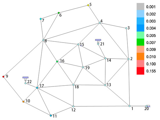
Figure 1.
Expected distribution of the nodal DFR.
3.2. Cases of Pipe Importance Assessment
DFR and DGR can quantify the safety level of the WDS. From the perspective of the management department, they want to know the importance of every pipeline. The following two cases introduce the calculation of the pipelines’ impact degree.
3.2.1. Case of Global UIPF
Anytown model is used in this section to analyze pipelines’ influence in the WDS. The pressures , are used in the pressure-driven model. In the simulation, the UIPF is marked with different colors according to Equation (13). Considering UIPF of pipelines for the whole WDS, there are eight pipelines (marked in orange and red) with UIPF of 0.01 or higher. The key pipeline is the outlet pipe of the southwestern pool, the UIPF of which is 0.155. The second one is the outlet pipe of the southern water pool, and the UIPF value is 0.031. Water outlets of the pool and the water plant play the most important roles for the entire area, so failure will have a significant impact on customers in the WDS. The UIPFs of pipelines in the center of the pipeline network are low in Figure 2. It is because that the nodes’ demands in this area are supplied by multiple pipes and one pipeline’s failure has little impact. As a result of the UIPF, Figure 2 demonstrates this phenomenon very well.
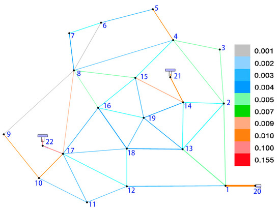
Figure 2.
UIPF assessment of Anytown network.
3.2.2. The Local and the Global UIPF of Real-Life WDS
(1) The Global UIPF of WDS
This case introduces that the local UIPF is different from that of the global for different evaluation areas. The result of the UIPF in the whole WDS is shown in Figure 3. From the perspective of the UIPF, there are 13 pipes (marked in orange and red) with a UIPF of 0.01 or higher in this case. Among them, the southern water plant outlet Pipe a (1400 mm) is with the highest UIPF of 0.088 (marked in red). This pipeline is the main outlet pipe of the southern water plant, and plays a key role in the southern region. The failing of Pipe a will have a significant impact on customers’ water consumption in its water distribution area, and the calculation result shows this phenomenon well. Meanwhile, it demonstrates that the UIPF of outlet Pipe b in charge of the southwest is not high, because the flow of Pipe b is only 370 m3/h, which accounts for 9.8% of the total outflow of the southern water plant. The water consumption in the southwest region is low, so the failure of Pipe b has little effect on the whole WDS. It shows that the importance of the pipeline is closely related to the downstream demand. The overall evaluation results visually identify the pipes with a high impact on the whole WDS. The above result can be used by the management to evaluate the hydraulic safety of the WDS.
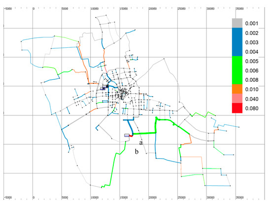
Figure 3.
The global UIPF of WDS.
Equation (13) can be applied in a local area too. The assessment result in a local area can show a distinction between the UIPFs of pipelines in a local area. The UIPF in the local area can be effectively expressed only in the evaluation of the local area with a clear distinction. If the UIPF is evaluated in the WDS, the distinction of the UIPFs of the pipelines is not high.
(2) The local UIPF in the northwest region
In the analysis of the node DGR expectation, the pipe network in the northwest region is firstly analyzed, and the UIPF is marked in different colors in Figure 4. It can be clearly identified from the figure that Pipe c (600 mm) and Pipe d (800 mm) are the key pipes, of which Pipe c’s UIPF is 0.105 and Pipe d’s UIPF is 0.127. These two pipes are the primary channels of the northwestern area. If an accident occurs, the water consumption in the northwest area will be greatly affected. In contrast, even if the surrounding pipes’ diameters are larger than these two pipes, the UIPFs are not higher. The water consumption in the area will not be greatly affected by the failure. This case shows that the diameter of the pipe is not the only factor that affects the UIPF of the pipeline, and the UIPF of the pipeline in the key area is higher than that of the thick ones.
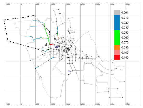
Figure 4.
UIPF assessment in the northwestern region of J city.
(3) The local UIPF in the southeast region
The southeast region is the region with the lowest level of the nodes’ DGR, and the evaluation result is shown in Figure 5. The UIPF assessment results show that the key pipeline is the outlet Pipe a of the southern water plant, with a UIPF of 0.376. This shows that Pipe a is the main pipeline for supplying water to the southeast region and it is very important to ensure its normal state. It is noteworthy that the green Pipe e with a larger pipe diameter is not one of the key pipes in this area. Pipe e’s UIPF is only 0.02, while the UIPFs of several small-diameter pipes downstream are higher. The reason is that Pipe e is not a unique channel for downstream customers. Although the diameter of Pipe e is large, its UIPF is not high for the local evaluation area downstream. The pipes closer to the customers downstream are more important than Pipe e.
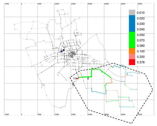
Figure 5.
UIPF assessment in the southeast region of J city.
The region in Figure 6 can be separated into two Areas A and B. Both areas are analyzed independently. When Pipe f fails, it will cause a significant impact on the water demand in this area. For Area A, the UIPF of Pipe f is high to 0.4. For the downstream of Pipe f, the UIPF is 1.
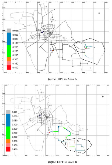
Figure 6.
Analysis of the UIPF in local area of J city.
Pipes g and h in Area B in the southeast have high UIPFs of 0.32 and 0.33, respectively. They are key pipelines for this region. The two pipelines satisfy about 70% demand independently; when either of them fails, customers in the area can also obtain water from the other pipelines, thus their impact degree is lower than that of the unique Pipe f in Area A. Between Pipes i and j connecting this area, the UIPF of the green Pipe i in the north is higher than that of the blue Pipe j in the south. It can be preliminarily considered that the green pipe is more important for water delivery. Similarly, the UIPF of the southern water plant’s outlet Pipe a is still very high, and its value reaches 0.46, which is higher than that in Area A. It is indicated that the pipeline has a greater impact on water distribution in Area B.
4. Conclusions
The water demand guarantee rate (DGR) and the water demand failure rate (DFR) are proposed to assess the safety of a Water Distribution System (WDS) in this paper. The mathematical expectation of DGR and DFR can describe the average safety level of the WDS. Based on the influence of pipe failure on water consumption, the Unit Influence of Pipe Failure (UIPF) is proposed to describe the relative importance of the pipelines in the system. The UIPF demonstrates the relative importance of pipelines based on water consumption in evaluation areas. Thus, it can be used to evaluate the impact of the pipeline’s failure, not only for the whole WDS but also for the local areas. UIPF’s advantages are that it can be used for both the local system and the global system, and it can improve the discrimination of pipe importance. It is a simple and intuitive indicator to describe the relative importance of various pipelines in large-scale and complex pipe networks. Even if experience can help public utility managers to judge the importance of pipelines, the UIPF provides a very important reference for them to make decisions, especially for those managers who lack professional experience and relevant technical background. The UIPF provides an important reference for the formulation of design, monitoring, and maintenance strategy for the WDS. It is beneficial to ensure safety and reasonable budget allocation. All cases show that UIPF can help the researchers find key pipelines in the WDS easily. It is an effective index to help the water management department make the plan for improving the safety level according to the importance of the pipelines.
Author Contributions
Conceptualization, W.C.; Data curation, G.X.; Investigation, Z.Z. and Z.L.; Methodology, Y.S.; Writing—original draft, Y.S. and X.Z.; and Writing—review and editing, W.C. All authors have read and agreed to the published version of the manuscript.
Funding
This research received National Nature Science Foundation of China (NSFC Project No. 51578486) and the Guangzhou Science and Technology Program (No. 201604020019).
Conflicts of Interest
The authors declare no conflict of interest.
Glossary
| WDS | Water distribution system |
| DGR | Water demand guarantee rate |
| DFR | Water demand failure rate |
| UIPF | Unit influence of pipe failure |
| The expression of the DGR | |
| The discretization result of the DGR | |
| Available flow in region S at time T | |
| The demand in area S at a specific T domain | |
| The DFR of node n when there is no pipeline failure in the WDS | |
| The probability of no pipeline failure in the pipeline network | |
| The probability of the pipeline i failing | |
| The DFR of node n when there is only component i failing | |
| The probability of pipeline i and j failing at the same time | |
| The DFR of node n when pipeline i and j fail at the same time | |
| A failure subset which corresponds to an accident state | |
| The DGR of node n when the WDS is not in failure | |
| The DGR of node n when the subset fails | |
| The mathematical expectation of the DFR of node n | |
| The mathematical expectation of the DGR at node n | |
| The influence degree of pipeline i | |
| The actual consumption of customer j at the pipe i failure state | |
| The water demand of customer j | |
| The length (km) of pipe i. | |
| Unit influence of pipe failure | |
| Node actual available flow | |
| Node demand flow | |
| Node actual head | |
| Node demand head | |
| Node minimum service head | |
| Poisson distribution probability |
References
- Kanakoudis, V.; Tsitsifli, S. Potable water security assessment—A review on monitoring, modelling and optimization techniques, applied to water distribution networks. Desalin. Water Treat. 2017, 99, 18–26. [Google Scholar] [CrossRef]
- Tsitsifli, S.; Kanakoudis, V. Developing THMs’ Predictive Models in Two Water Supply Systems in Greece. Water 2020, 12, 1422. [Google Scholar] [CrossRef]
- Hongwei, L.; Mou, L.; Song, Y. The research and practice of water quality safety evaluation for Ji Nan urban water supply system. Procedia Environ. Sci. 2011, 11, 1197–1203. [Google Scholar] [CrossRef]
- Kanakoudis, V.K.; Tolikas, D.K. Assessing the performance level of a water system. Water Air Soil Pollut. Focus 2004, 4, 307–318. [Google Scholar] [CrossRef]
- Alperovits, E.; Shamir, U. Design of optimal water distribution systems. Water Resour. Res. 1977, 13, 885–900. [Google Scholar] [CrossRef]
- Tung, Y. Evaluation of water distribution network reliability. In Hydraulics and Hydrology in the Small Computer Age; ASCE: Reston, VA, USA, 1985. [Google Scholar]
- Khomsi, D.; Walters, G.A.; Thorley, A.; Ouazar, D. Reliability tester for water-distribution networks. J. Comput. Civ. Eng. 1996, 10, 10–19. [Google Scholar] [CrossRef]
- Wagner, J.M.; Shamir, U.; Marks, D.H. Water distribution reliability: Analytical methods. J. Water Resour. Plan. Manag. 1988, 114, 253–275. [Google Scholar] [CrossRef]
- Wagner, J.M.; Shamir, U.; Marks, D.H. Water distribution reliability: Simulation methods. J. Water Resour. Plan. Manag. 1988, 114, 276–294. [Google Scholar] [CrossRef]
- Kansal, M.L.; Kumar, A.; Sharma, P.B. Reliability analysis of water distribution systems under uncertainty. Reliab. Eng. Syst. Saf. 1995, 50, 51–59. [Google Scholar] [CrossRef]
- Guercio, R.; Xu, Z. Linearized optimization model for reliability-based design of water systems. J. Hydraul. Eng. 1997, 123, 1020–1026. [Google Scholar] [CrossRef]
- Shinstine, D.S.; Ahmed, I.; Lansey, K.E. Reliability/availability analysis of municipal water distribution networks: Case studies. J. Water Resour. Plan. Manag. 2002, 128, 140–151. [Google Scholar] [CrossRef]
- Yazdani, A.; Jeffrey, P. Applying network theory to quantify the redundancy and structural robustness of water distribution systems. J. Water Resour. Plan. Manag. 2012, 138, 153–161. [Google Scholar] [CrossRef]
- Berardi, L.; Laucelli, D.B.; Simone, A.; Mazzolani, G.; Giustolisi, O. Active leakage control with WDNetXL. Procedia Eng. 2016, 154, 62–70. [Google Scholar] [CrossRef]
- Kanakoudis, V.; Tsitsifli, S. Water pipe network reliability assessment using the DAC method. Desalin. Water Treat. 2011, 33, 97–106. [Google Scholar] [CrossRef]
- Tanyimboh, T.; Tahar, B.; Templeman, A. Pressure-driven modelling of water distribution systems. Water Sci. Technol. Water Supply 2003, 3, 255–261. [Google Scholar] [CrossRef]
- Seyoum, A.G.; Tanyimboh, T.T. Investigation into the Pressure-Driven Extension of the EPANET Hydraulic Simulation Model for Water Distribution Systems. Water Resour. Manag. 2016, 30, 5351–5367. [Google Scholar] [CrossRef]
- Su, Y.C.; Mays, L.W.; Ning, D.; Lansey, K.E. Reliability-Based Optimization Model for Water Distribution Systems. J. Hydraul. Eng. 1987, 113, 1539–1556. [Google Scholar] [CrossRef]
- Tanyimboh, T.; Sheahan, C. A maximum entropy based approach to the layout optimization of water distribution systems. Civ. Eng. Environ. Syst. 2002, 19, 223–253. [Google Scholar] [CrossRef]
- Cullinane, M.J.; Lansey, K.E.; Mays, L.W. Optimization-availability-based design of water-distribution networks. J. Hydraul. Eng. 1992, 118, 420–441. [Google Scholar] [CrossRef]
- Tabesh, M.; Jamasb, M.; Moeini, R. Calibration of water distribution hydraulic models: A comparison between pressure dependent and demand driven analyses. Urban Water J. 2011, 8, 93–102. [Google Scholar] [CrossRef]
- Reddy, L.S.; Elango, K. Analysis of water distribution networks with head-dependent outlets. Civ. Eng. Syst. 1989, 6, 102–110. [Google Scholar] [CrossRef]
- Germanopoulos, G. A technical note on the inclusion of pressure dependent demand and leakage terms in water supply network models. Civ. Eng. Syst. 1985, 2, 171–179. [Google Scholar] [CrossRef]
- Rossman, L. EPANET 2 Users Manual; Cincinnati US Environmental Protection Agency National Risk Management Research Laboratory: Cincinnati, OH, USA, 2000; Volume 19, pp. 115–118. [Google Scholar]
- Fujiwara, O.; Li, J. Reliability analysis of water distribution networks in consideration of equity, redistribution, and pressure-dependent demand. Water Resour. Res. 1998, 34, 1843–1850. [Google Scholar] [CrossRef]
- Liu, J.L.; Chen, X.; Zhang, T.J. Application of time series-exponential smoothing model on urban water demand forecasting. Adv. Mater. Res. 2011, 183–185, 1158–1162. [Google Scholar] [CrossRef]
- Goulter, I.C.; Coals, A.V. Quantitative approaches to reliability assessment in pipe networks. J. Transp. Eng. 1986, 112, 287–301. [Google Scholar] [CrossRef]


© 2020 by the authors. Licensee MDPI, Basel, Switzerland. This article is an open access article distributed under the terms and conditions of the Creative Commons Attribution (CC BY) license (http://creativecommons.org/licenses/by/4.0/).