Modelling of Surface Runoff on the Yamal Peninsula, Russia, Using ERA5 Reanalysis

Abstract

The Yamal peninsula is a territory of active industrial development as it contains several rich fields of natural condensed gas and oil. The density of the gullies net on the Yamal peninsula is one of the highest in the Russian Arctic. The natural environment or constructions can be potentially damaged by gully erosion and the cost of such damage is high. The models of gully erosion require surface runoff estimates. The hydrological model was developed for surface runoff estimation during the spring snow thaw and summer rains. In the conditions of Arctic climate with deep permafrost, the losses in runoff are limited to evaporation, as soil permeability is negligible. The model was calibrated on the available measurements. The meteorological base for hydrological calculations was ERA5 reanalysis, the fifth generation of European Centre for Medium-Range Weather Forecasts (ECMWF) atmospheric reanalyses, validated on the meteorological data. The deviations of reanalysis data from the measurements cause the errors in the results of surface runoff calculation. The daily surface runoff can vary in the range of 18–30% due to ERA5 errors in air temperature and snow cover depth. As the daily surface runoff is the main input to the models of gully erosion, these errors must be taken into account in the modelling of gully erosion on the Yamal peninsula.

1. Introduction

The Yamal peninsula is a broad territory in the Russian Arctic, bounded by Baidaratskaya Bay from the west, Kara Sea from the north, Ob Bay from the east, and the Ob river valley from the south. The area of the peninsula is 122,000 km² with the length from south to north 750 km and the width 140–240 km [1]. It extends along the longitudes 67–73° E between the Arctic Circle (66.56° N) and the latitude 73° N (Figure 1). Despite the severe climate, fragile forestless tundra landscape and deep permafrost, this land is the territory of active industrial development as it contains several rich fields of natural condensed gas and oil. The main reason is that the world energy budget cannot be closed without this source of hydro-carbonates [2,3,4,5,6].

At the same time, the meteorological and hydrological regime measurements for the Yamal peninsula are completely inadequate to the rates of territory development. There are 7 meteorological stations on the peninsula and surrounding lands at present, and it was never more than 11 working stations simultaneously. The short sequences of hydrological measurements are available only from 3 points in the area of 122,000 km² [7,8,9].

The density of river, dry valleys and gullies net on the Yamal peninsula is one of the highest in the Russian Arctic–the maximum density of stable and active gullies is 1–2 km/km² here [10]. Therefore, the natural environment or constructions can be potentially damaged by gully erosion and the cost of such damage is high. The potential of gully erosion can be estimated with the existing models [10,11,12,13,14], but all these models require the estimates of the surface runoff. In the situation of a nearly complete absence of measurements of the surface runoff, the only way to obtain such information for the entire Yamal peninsula is the hydrological modelling on the base of meteorological data.

Meteorological data are widely used as inputs for hydrological modelling. The most accurate data source is the weather stations, but there are many regions with sparse weather stations coverage, which causes limitations of hydrological studies.

Several studies use remote sensing data for hydrological modelling in various areas. For example, in [15] satellite-based precipitation data were included as an input for hydrological modelling in arid and inaccessible watersheds in Pakistan. In [16] the combination of weather radar data on rainfall with rain-gauge data were applied for hydrological modelling in the United Kingdom.

However, the results obtained in papers on this subject showed that remote sensing data needed error corrections and can be used only for regions with dense stations cover. In the regions where the distribution of weather stations is sparse or weather stations are absent, reanalysis may provide a good alternative to station data. Reanalyses have global coverage and using weather forecast model they assimilate observations from a wide variety of sources (weather stations, radiosondes, aircraft, satellites, buoys, ships, etc.). The quality of various reanalysis datasets was evaluated in many studies where data from reanalyses were compared with weather station data in several regions of the world [17,18,19,20,21].

Furthermore, several studies using reanalyses and gridded datasets for hydrological modelling compared them to observations. The comparison indicated that reanalyses perform better than gridded observations when the weather stations density is low [22,23,24,25].

Reanalyses are widely used for hydrologic applications, in particular for hydrologic modelling in the regions with sparse data. For example, in [26] ERA5 reanalysis (the fifth generation of European reanalysis) was evaluated and used for annual water budget in two basins in India. In [27] data from ERA-Interim and WFDEI Reanalyses were applied as input for hydrological modelling in the data-scarce Sudano-Sahel region. In [28] CFSR reanalysis data were used for modelling over five watersheds in different hydroclimate regimes in the United States. In [29] NARR, ERA-Interim, CFSR, and MERRA reanalyses data were used for the calibration of the hydrological model and for the simulation of river flows over 370 watersheds in the continental part of the United States. In [30] operational runoff forecasting systems were developed for early warnings of floods and flashfloods for the European part of Russia using ERA-Interim reanalysis. In [31] five datasets and reanalyses were tested and used for the modelling of discharges in the Mekong river basin. Benefits of ERA-Interim reanalysis rainfall application for runoff modelling at monthly time scale in not enough gauged catchments was shown in [32] for the Mekong and Red River Basins. The hydrological model for a mountain basin in Patagonia was developed in [33]. The ERA-Interim soil moisture was compared with surface soil moisture from hydrological measurement network over southeast Australia [34], and it was demonstrated that the ERA-Interim soil moisture shows good agreement with in situ soil moisture values, required for water cycle modelling.

The main purpose of the presented work is the calculation of the surface runoff characteristics for the entire Yamal peninsula. The hydrological model of surface runoff estimation was developed, calibrated, and used for this purpose. The meteorological base for hydrological calculations was the reanalysis, particularly ERA-5. The reanalysis data were validated on the available meteorological measurements for this region before being used for hydrological modelling. There are possible errors in surface runoff estimations due to the deviation of reanalysis data from the measurements. These errors must be taken into account in the further modelling of gully erosion processes on the Yamal peninsula.

2. Materials and Methods

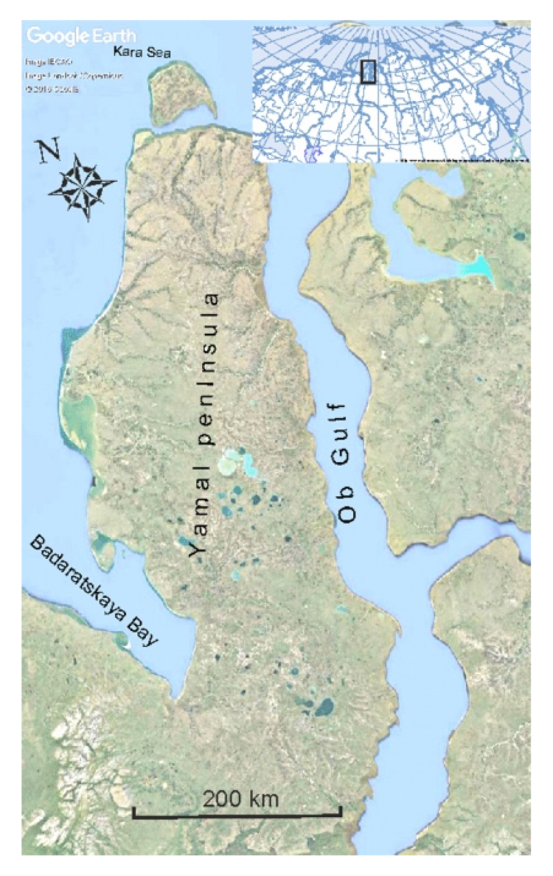
2.1. Climatic and Hydrological Characteristics of Yamal

2.1.1. Climatic Characteristics

The study region has specific climatic features determined by the combination of various factors: the geographical position, solar radiation regime, atmospheric circulation, underlying surface. To make further assessments of the ERA5 reanalysis ability to reproduce meteorological characteristics and to simulate the hydrological parameters (Section 3), it is necessary to understand in more detail the climatic features of the study area.

The climate of the Yamal peninsula is determined by its latitudinal position, the proximity of marine areas, and the influence of the south of the mainland. The Yamal peninsula is characterized by a cold and humid climate and extends in the Arctic (northern part of the peninsula) and Subarctic (southern part of the peninsula) zones, according to B.P. Alisov’s climatic zoning scheme, and so-called polar climate of the tundra, according to V. Keppen’s classification [35].

The cold season is very severe because of the combination of low temperatures with strong winds. The average temperature in January in different parts of Yamal peninsula is −22~−25 °C (Figure 2a). Over the past 30 years, winters became warmer on the Yamal peninsula and in the adjacent areas. This fact was also noticed in [36]. The spatial distribution of linear trends of air surface temperature (Figure 2b) shows the warming at a rate of 0–2.2 °C per decade on average, the rate increases towards the north.

In July–August, the average air temperature near the surface is approximately 6~8 °C (Figure 2c). Summer warming long-term trends (Figure 2d) are much slower than the winter ones (Figure 2b), the mean rate of temperature growth is below 0.5 °C per decade and only in the north of Yamal linear trend is about 0.7~0.8 °C.

The seasonal cycle of surface air temperature at 2m is shown in Figure 3. There are data of four meteorological stations located on the west coast of Yamal (Harasavey is the northern station, Marresale is more southern one), on its east coast (Tambey) and in the south of peninsula (Novy Port) from RIHMI-WDC archive [37] and data by A. Vasiliev et al. [38].

All these stations show a significant seasonal cycle of surface air temperature. On the Yamal peninsula, winter temperature decreases towards the northeast. Summer temperature changes zonally.

The excessive moisture is typical for Yamal. The average annual precipitation is about 300 mm; the estimated annual evaporation is 200 mm.

Snow cover on Yamal persists for approximately 260 days per year. Since the formation of a stable snow cover, its height gradually increases. The most intense increase in snow depth occurs in the period from the second half of November until the beginning of January when the precipitation is significant due to the most frequent cyclonic weather. In late January and February, the increase in snow height is weakening. Snow cover reaches its maximum height in the third decade of April—the first decade of May. The density of the snow cover gradually increases during the winter. The maximum snow density is reached in the spring, before the snow melts.

2.1.2. Hydrological Characteristic

There are no long-term hydrological measurements on the rivers of the Yamal peninsula. The main information was collected by several expeditions of various organizations, which took place in the 1965–1997 for local purposes. Of greatest interest for our study are measurements taken by the expeditions of State Hydrological Institute (Saint-Petersburg) and of Moscow State University at three points (Figure 4) on several small river basins during the years 1985–1993. We used these measurements of river runoff during the period of snow thaw [7] and surface runoff during the snow thaw and summer rains [8,9] for calibration of the calculations with the hydrological model.

The only example of spatial distribution of river runoff characteristics on the territory of the peninsula is described in [7]. It was based on the measurements at the meteorological stations and aircraft surveys [39]. The surface runoff regimen depends on the size of the contributing basin. On the slope’s runoff begins practically synchronous to the snow thaw, the maximum river runoff of the small rivers with the basin area less than 400 km² occurs 4–5 days after the beginning of snow thaw. The surface runoff during the summer rains with low intensity can be negligible. After a few days with low intensity rains, the rain with 10–20 mm daily depth often follows. Such rain produces the surface runoff volume practically equal to the volume of rainfall for a catchment, with the maximum runoff 1–3 h after the maximum rainfall [40].

2.2. Data

2.2.1. Station Data and ERA5 Reanalysis

In this paper, we evaluate the quality of ERA5 reanalysis using in situ observational data from seven meteorological stations located on the Yamal peninsula and in the adjacent areas.

Reanalysis provides four-dimensional gridded data on surface and upper-air parameters. It combines observational data assimilation system and a forecast model. It covers a long period and can be used for a wide range of applications (including hydrological ones [28]). In this study, the reanalysis data provided input data for the hydrological model that are highly sensitive to the input conditions. It makes an evaluation of reanalysis data against available independent observational data a very important task.

ERA5 is a new climate global reanalysis dataset produced by the European Centre for Medium-Range Weather Forecasts (ECMWF). ERA5 has several significant improvements compare to previous ECNWF Reanalysis ERA-Interim [41]: an increase of the horizontal grid spacing, of the number of vertical levels, of the temporal resolution, and of number of observations assimilated. The vertical resolution of ERA5 contains 137 pressure levels from 1000 hPa to 1 hPa. The ERA5 has an hourly temporal resolution.

As observational data, we use seven meteorological stations from the RIHMI-WDC archive [37]: 1. Marresale, 2. Antipayuta, 3. Tazovsk, 4. Novy Port, 5. Salekhard, 6. Nadym, 7. Nyda (Figure 4). Please note that the datasets of these stations are representative (gaps in data are less than 10%) and include daily data on air temperature, precipitation, and snow height. The Tambey and Harasavey stations used for Figure 3 were excluded from the current assessment due to missing precipitation and snow data. The nearest corresponding ERA5 reanalysis grid points have almost the same coordinates as stations (Figure 4), therefore we prefer not to make data interpolation from grid points to the coordinates of stations. We use only land-located ERA5 grid points.

We evaluate the ERA5 Reanalysis data quality in accordance with the features of the hydrological model used in this study, including the air temperature near surface (at 2 m), precipitation, and snow height. We divide a year into three periods. The period of snow thaw begins from the stable mean daily temperature above 0 °C in spring and ends when snow cover totally disappears. The next period of summer rains lasts from the end of the period of snow thaw until the mean daily temperature drops below 0 °C and the snow cover appears. Cold period lasts from the end of the summer rains period to the beginning of snow thaw. These periods were identified for each station and for the nearest grid point.

The error analysis applied in this paper contain bias, root mean square error (RMSE), the correlation coefficient (r), ratio of standard deviations (standard deviation of ERA5 reanalysis divided by the one from the meteorological station data) (STD ratio). The lower RMSE corresponds to the closest reproduction of values by ERA5. STD ratio (reanalysis divided by observed) shows the correspondence of ERA5 data variability to the observed one. Values above 1 indicate an overestimated variability, and vice versa. This statistic criterion is important for the hydrological model because the variability has generally impact on the snow melting rate. Here we focus on the period 1985–2019 for evaluation.

2.2.2. Hydrological Model Description

In the conditions of Arctic climate with deep permafrost and high density of linear erosion features hydrological modelling bears specific characteristics, described further. Two main sources of water flow are typical for this environment: snow thaw during the spring and rainfall mostly during the summer.

The Period of Snow Thaw

The melt coefficient approach (also called the melt factor, degree-day-factor, or degree-day ratio) was used for calculation of runoff depth Xs for the period of snow thaw. This type of modelling was designed in the years 1956–1969, and its effectiveness is well known [42,43]. The current version (Figure 5) is the combination of the models [44,45,46,47], using maximum depth of snow pack Hs (as water equivalent), precipitation P, air temperature T and evaporation E values from reanalysis. The main procedures describe step-by-step changes of the amount of snow Hs (water equivalent) and of water Hw_in_s in the snowpack H during time interval Δt for each time step between t_j and t_j+1 (at time t_j+1/2). Here index “s” means “snow”, index “w”–“water”, “w_in_s”–water in snow, “w_to_s” and “s_to_w”–exchange by water and snow in the snow pack.

When the air temperature is negative or zero $(T_{j+1/2}\le 0)$, water in snowpack (if available) freezes. According to empirical data of Komarov et al. [44],

$$\mathrm{If} {\left(Hw\_in\_s\right)}_j\ge k_f\sqrt{\left|T\right|}\Delta t \mathrm{then} {\left(Hw\_to\_s\right)}_{j+1/2}=k_f\sqrt{\left|T\right|}\Delta t$$

(1)

$$\mathrm{If}{\left(Hw\_in\_s\right)}_j<k_f\sqrt{\left|T\right|}\Delta t \mathrm{then} {\left(Hw\_to\_s\right)}_{j+1/2}={\left(Hw\_in\_s\right)}_j$$

(2)

$${\left(Hw\_in\_s\right)}_{j+1}={\left(Hw\_in\_s\right)}_j-{\left(Hw\_to\_s\right)}_{j+1/2}$$

(3)

$${\left(Hs\_to\_w\right)}_{j+1/2}=0$$

(4)

As the result, amount of snow in the snow pack increases by freezing water and by snow precipitation, but decreases by snow sublimation (both taken from ERA-5)

$${\left(Hs\right)}_{j+1}={\left(Hs\right)}_j+{\left(Hw\_to\_s\right)}_{j+1/2}+P_{j+1/2}-E_{j+1/2}+$$

(5)

Runoff is not formed in this case

$${\left(Xs\right)}_{j+1}=0$$

(6)

When the air temperature is above zero $(T_{j+1/2}>0)$, snow in snowpack melts with the rate controlled by melt coefficient k_sm:

$${\left(Hs\_to\_w\right)}_{j+1/2}=k_{sm}T\Delta t$$

(7)

The amount of water in snow also increases if precipitation occurs

$${\left(Hw\_in\_s\right)}_{j+1/2}={\left(Hw\_in\_s\right)}_j+{\left(Hs\_to\_w\right)}_{j+1/2}+P_{j+1/2}$$

(8)

Accordingly, the amount of snow in the snowpack decreases

$${\left(Hs\right)}_{j+1/2}={\left(Hs\right)}_j-{\left(Hs\_to\_w\right)}_{j+1/2}$$

(9)

Vinogradov [45] proposed that there is a critical proportion of water in snow βws_max, which depends on density of snow γs

$$\beta wc\_\max =k_{wc}\left(\frac{920}{\gamma s}-1\right)$$

(10)

If proportion of water in snow $\beta \_wc$

$${\left(\beta \_wc\right)}_{j+1/2}={\left(Hw\_in\_s\right)}_{j+1/2}/{\left(H\right)}_j$$

(11)

is less than critical $\beta wc\_\max$, runoff is not formed

$${\left(Xs\right)}_{j+1}=0$$

(12)

and snow pack depth at the beginning of the next time step is

$${\left(H\right)}_{j+1}={\left(Hs\right)}_{j+1/2}+{\left(Hw\_in\_s\right)}_{j+1/2}-E_{j+1/2}$$

(13)

When proportion of water in snow $\beta \_wc$ is more than critical, then part of water in snow forms runoff as proposed by Vinogradov [45]

$${\left(Xs\right)}_{j+1/2}={\left(Hw\_in\_s\right)}_{j+1/2}\begin{array}{cccc}\left[{\left(\beta \_wc\right)}_{j+1/2}-\beta \_wc\_\max \right]& & & \end{array}$$

(14)

In this case, water content in snow pack at the beginning of the next time step is

$${\left(Hw\_in\_s\right)}_{j+1}={\left(Hw\_in\_s\right)}_{j+1/2}-{\left(Xs\right)}_{j+1/2}$$

(15)

and snow pack depth

$${\left(H\right)}_{j+1}={\left(Hs\right)}_j-{\left(Hs\_to\_w\right)}_{j+1/2}+{\left(Hw\_in\_s\right)}_{j+1}-E_{j+1/2}$$

(16)

Snow thaw period finishes when

(Xs)_j = 0

(17)

The initial snow pack depth H = Hs has irregular pattern on the catchment. Snow is driven by wind during the winter and accumulates in depressions (river and gully valleys), near steep slopes, and in dense vegetation. The measurements on the gullied territory of the west-central Yamal peninsula [8] showed the typical distribution of snow depth/mean snow depth ratio (Nratio) at the beginning of snow thaw period. The spatial changes in snow cover depth are described by gamma-distribution

$$p\left(Nratio\right)=\frac{1}{\mathsf{\Gamma }\left(\alpha \right){\beta }^{\alpha }}Nrati{o}^{\propto -1}\exp \left[\frac{Nratio}{\beta }\right]$$

(18)

Here $\alpha ={\left(\frac{mean}{\sigma }\right)}^2; \beta =\frac{{\sigma }^2}{mean}$, Γ is gamma function.

For the gullies of the west-central Yamal with mean Nratio = 1 and σ = 0.29 the parameters of gamma distribution are: α = 11.64 and β = 0.085. To take into account the uneven thickness of the snow cover, the runoff depth Xs was summarized with different values of Nratio for each period, weighted with probabilities from Equation (18).

The Period of Summer Rains

The runoff depth for the period of summer rains Xr during time Δt was taken equal to rainfall depth P(t). Evaporation E and infiltration for the periods with rainfall were assumed to be 0, and the losses consisted of filling depressions on the catchment surface. Water filled these depressions during the rainfall to the depth H_fill and evaporated from them during the periods between rainfalls. The algorithm of calculating the losses with the formula of Popov [48] is as follows:

$${\left(H_{fill}\right)}_{j+1}={\left(H_{fill}\right)}_j+H_{f\max }\left[1-\exp \left(-\frac{P}{H_{f\max }}\right)\right]-E_{j+1/2}$$

(19)

when the water depth in depressions H_fill exceed its maximum value H_fmax, the excess form the surface runoff.

2.2.3. The Model Calibration

The melt coefficient k_sm was calibrated upon the measurements of the spring periods of 1992–1993, when both snow pack depth distribution and runoff were measured [8]. For k_sm = 1.25 × 10⁻⁴ the measured and calculated runoff depths were quite similar (Figure 6).

Here the coefficient of water content in snow k_wc was taken equal to 0.163 after Vinogradov [45] and the coefficient of water freezing k_f was taken equal to 1.85 × 10⁻⁵ after Komarov [44]. The error of estimate of daily runoff (in terms of standard deviation σ_E is about ±10 mm, this measure of an error will be used further in model sensitivity analysis.

The calibration of water depth in depressions $H_{fill}$ in Equation (19) is based on the only measured rain in August 1990, for which both rainfall and runoff depths were available [40]. The evaporation was taken from ERA5, and the model parameter $H_{f\max }$ = 22 mm fits well with these measurements.

3. Results

3.1. Evaluation of ERA5 Reanalysis Quality

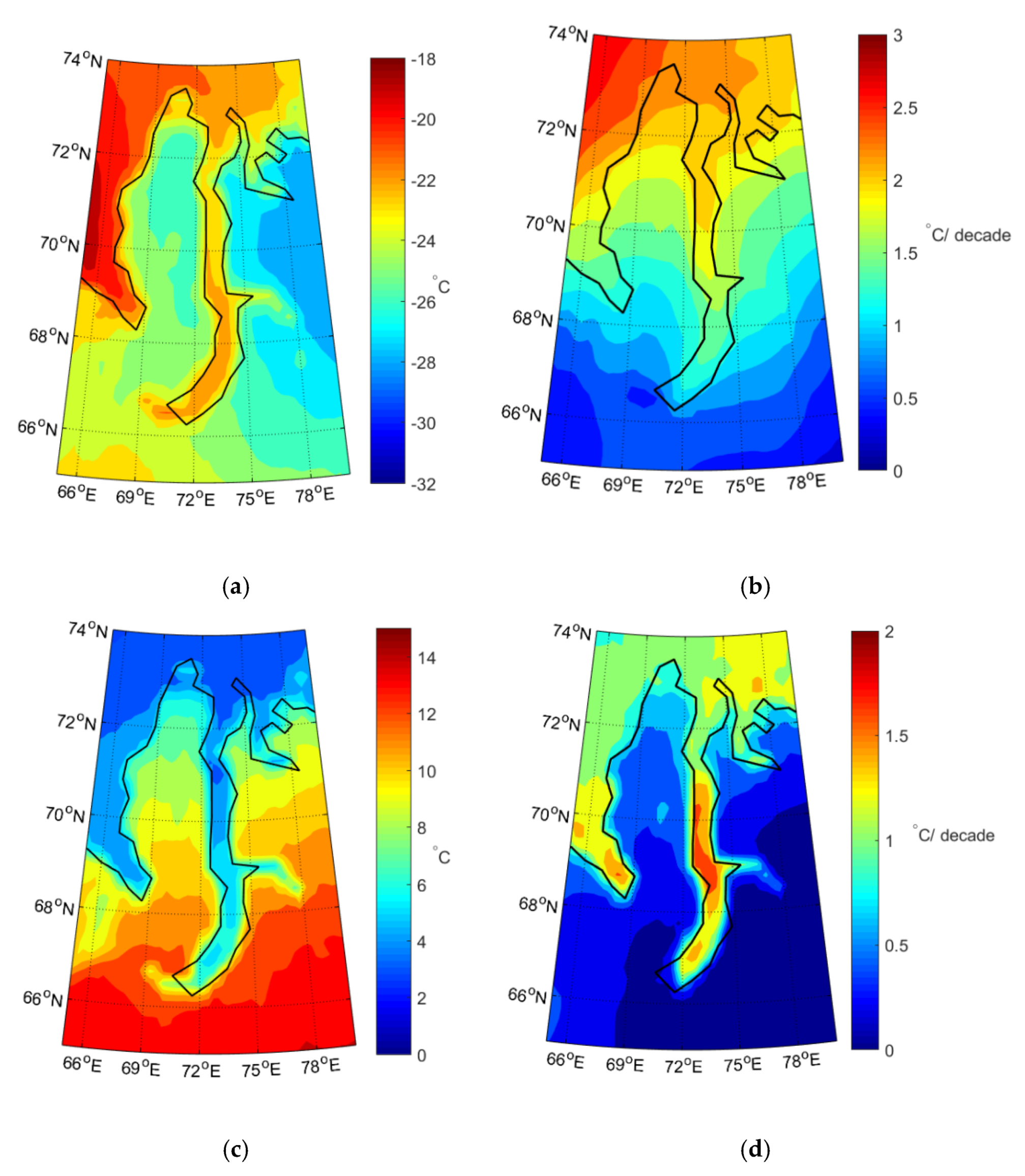
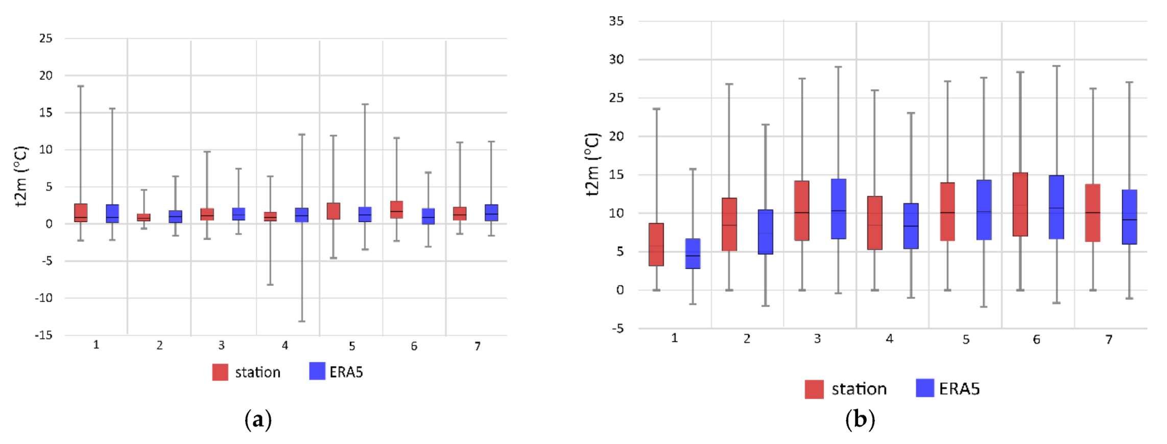
3.1.1. Surface Air Temperature

The error statistics for the surface air temperature at 2 m for snow thaw and summer rains periods are shown in Figure 7. The averaged observed 2 m air temperature varies from 1 °C to 2.7 °C in the period of snow thaw (Figure 7a) and from 6.3 °C to 11.3 °C in the summer rains period (Figure 7b). Errors of the maximum and minimum 2m temperature (box-whiskers) do not show a unidirectional tendency. The difference between ERA5 and observed mean values is no more than 0.4–0.6 °C (except at Nadym in the period of snow thaw, where it is about 1.3 °C, and Marresale in summer rains period, where it is about 1.4 °C). In general, ERA5 slightly underestimates mean 2 m air temperature compared to the station data.

RMSE is higher during the summer rains period (Figure 8a, green) than in the period of snow thaw (Figure 8a, orange). The maximum RMSE in the summer rains season is found for Marresale (2.5 °C), and in the period of snow thaw the worst representation of 2 m air temperature is revealed at Nadym (1.7 °C).

The correlation analysis shows high correlation coefficients in the summer rains period (above 0.9). The correlation coefficients are very close to 1 at the Tazovk, Salekhard, and Nadym stations (Figure 8b, green). In the period of snow thaw the correlation coefficients are slightly lower but generally higher than 0.8 (except Novy Port where the coefficient is only 0.68) (Figure 8b, orange).

In the period of snow thaw, reanalysis significantly (1.5–1.6 times) overestimated the variability for Novy Port and Antipayuta stations and underestimated it for Marresale (See Figure 8c for STD ratio, orange). In the summer rains period, in general, the strong overestimations/underestimations in variability do not occur (the ratio is close to 1), except for Marresale, where the variability is underestimated by reanalysis (Figure 8c, green).

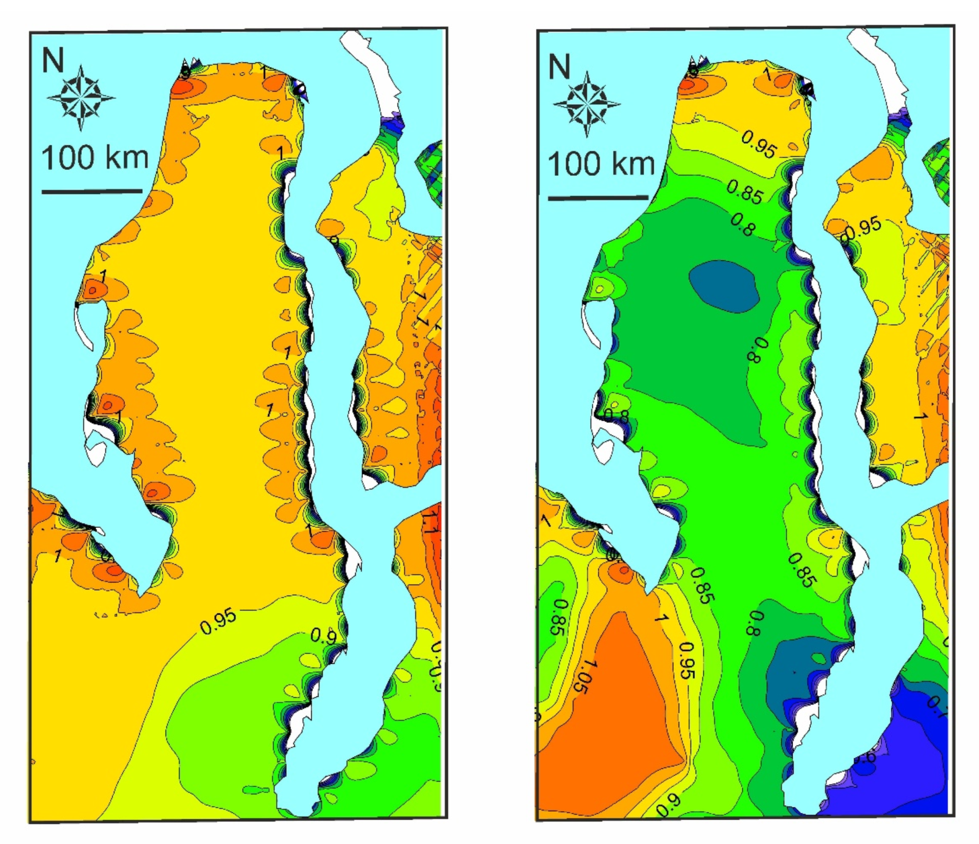
3.1.2. Precipitation

Figure 9 and Figure 10 show the error statistics for total daily precipitation. We analyze three periods (cold, snow thaw, summer rains) here, as all of them are very important for the hydrological model. We add an evaluation of extreme precipitation (95th percentile) because it shows the ability of reanalysis to reproduce extreme rainfall or snowfall.

It is well known that the precipitation is reproduced much worse in the reanalyses due to its uneven spatial distribution and local features [49,50], compared, for example, to the air temperature, especially in the high latitudes [17].

The mean values of daily precipitation are much less in the cold period (Figure 9a) to compare to the warmer periods–those of snow thaw (Figure 9c) and summer rains (Figure 9e). The largest differences between ERA5 and station data are registered at Antipayuta for the cold season and at Novy Port for summer rains and of snow thaw periods. Maximum values of daily precipitation are reproduced by ERA5 much worse than mean values (“whiskers” at box plots, Figure 9a,c,e).

As regards extreme precipitation, mean 95th percentile of daily precipitation varies from 2.1 to 5.9 mm in the cold period (Figure 9b), from 4.7 to 10 mm during the snow thaw (Figure 9d) and summer rains (Figure 9f) periods. ERA5 reanalysis overestimates it for all periods, but there are practically no discrepancies at some stations (Tazovsk, Salekhard, Nadym). This may be caused by the intracontinental position of these stations, since the spatial structure of precipitation there may be more uniform and therefore better reproduced by reanalysis.

The maximum RMSE is observed in the summer rains period (Figure 10a, green).

Correlations coefficients for daily precipitation (Figure 10b) are expectedly less compared to air temperature (Figure 8b), but still higher than 0.5. These correlation coefficients are independent from the period. The best correlation was found for Salekhard and Nadym (0.6–0.7).

In the period of snow thaw, ERA5 overestimates the variability of precipitation at the Novy Port station, for other stations, the STD ratio varies between 0.9 and 1.3 (Figure 10c, yellow). In the summer rains season, the variability at Antipayuta and Novy Port stations is overestimated by ERA5 (Figure 10c, green). In the cold period, the ERA5 variability of daily precipitation is less at Tazovsk and higher at Marresale and Antipayuta compared to observed values (Figure 10c, blue).

3.1.3. Snow Cover

Figure 11 and Figure 12 show the error statistics for the snow cover. We examine two characteristics of snow cover–maxima of snow height at the end of cold period and dates of these maxima. While mean snow height is reproduced in reanalysis data rather well, extreme values demonstrate less accordance with station data.

On average, the smallest maximum snow height is recorded at the Marresale station (28 cm), the highest snow height is observed at inland stations (70–90 cm) (Figure 11a). For most stations ERA5 overestimates the mean maximum snow heights (except for Nadym and Nyda stations). The maximum values in the most stations are less than 10 cm, except for Nyda station with strong difference between observed and ERA5 (about 30 cm). The minimum values aren’t reproduced correct but they are much less important for hydrological model.

The time series at several stations have a significant trend of the increase of maximum snow height at the end of cold season (confidence level of 95%)—20–22 cm per decade at Nyda and Tazovsk, 8–9 cm per decade at Salekhard and Novy Port. For estimations of errors, we removed linear trend from data from these stations and from the nearest grid points of ERA5 reanalysis. Figure 11b shows RMSEs for maximum snow height.

We also analyze the date of snow height maximum. The earliest maximum occurs at Salekhard and the latest one is observed at Marresale (Figure 12a). ERA5 reproduces the maximum snow height earlier at Tazovsk, Novy Port, Nadym, and Nyda compared to observations, for the other three stations ERA5 shows a lag of snow height maximum date no more than 5 days.

The time series of Salekhard and Nyda stations show significant linear trends (14 days and 9 days per decade, respectively). We removed trends them for analysis. Figure 12b shows RMSEs of the date of snow height maximum. RMSEs are rather high, about one month.

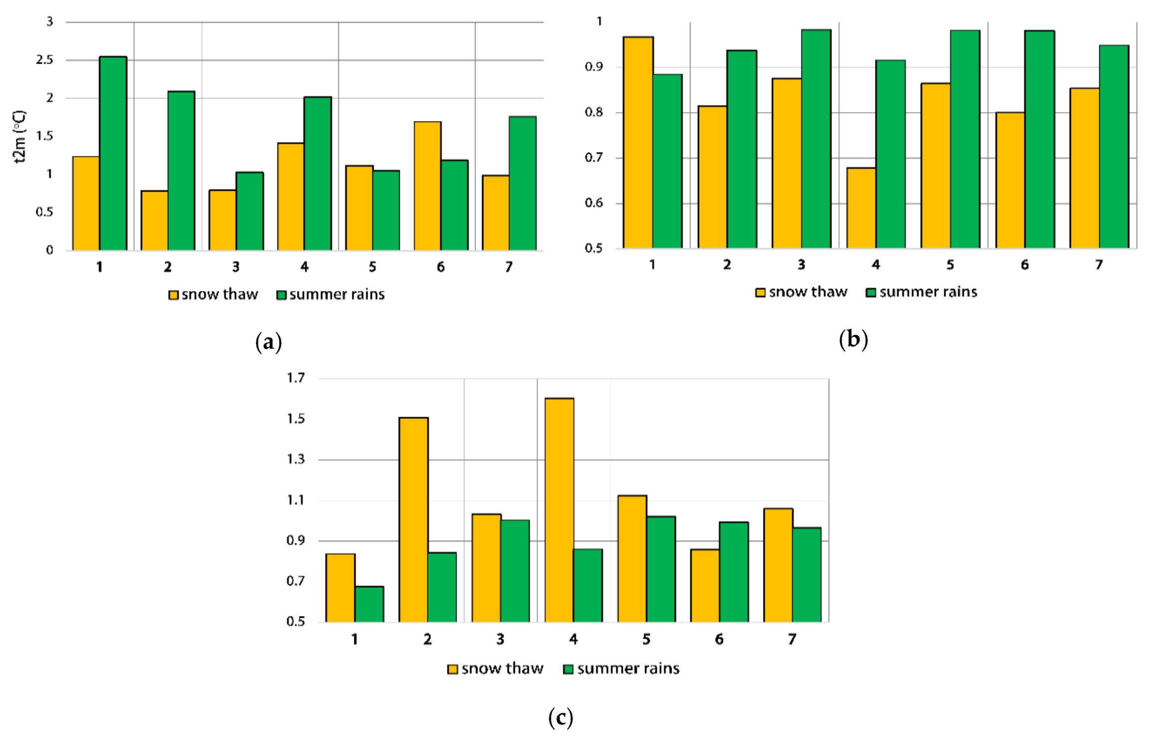
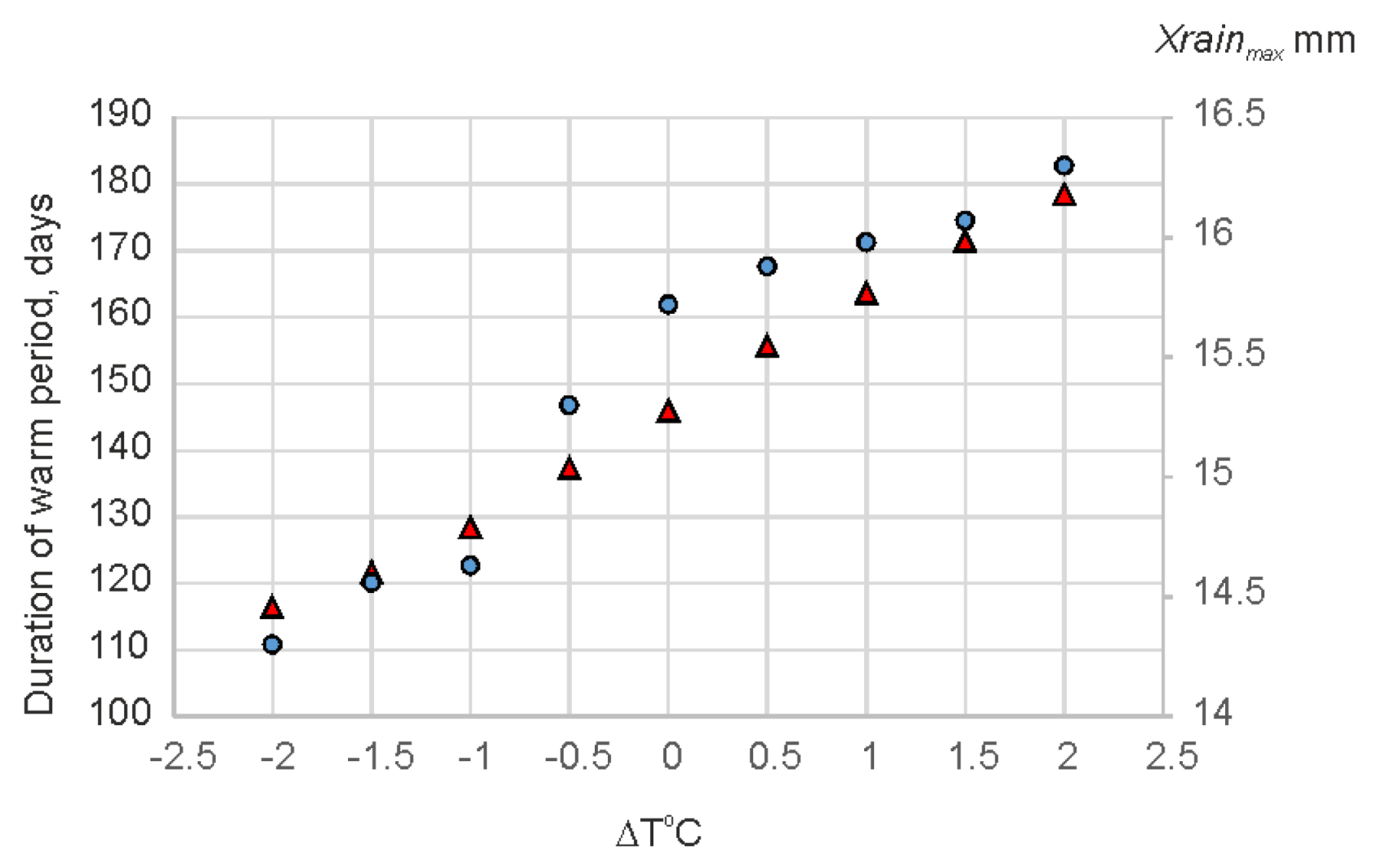
3.2. Model Sensitivity Analysis

3.2.1. Snow Thaw Period

Surface runoff depth is characterized by total runoff depth during snow thaw X_s, maximum daily runoff depth X_{s_max} and by the parameters of daily runoff probability functions. The calculations of these characteristics according to Equations (1)–(17) are controlled by snow pack depth (water equivalent) at the beginning of thaw period H_s, precipitation P, air temperature T, evaporation E and model coefficients of water content in snow k_wc, of water freezing k_f and melt coefficient k_sm. Additionally, the spatial distribution of snow pack depth is controlled by the parameters of gamma-distribution (Equation (18)) α and β (

Table 1. Range of temporal variation of model characteristics used in sensitivity analysis. The number of numerical experiments n = 1 + (Max − Min)/Step.

Model Characteristics, Varied in Sensitivity Analysis		Min	Max	Step
Input values	Snow depth at the beginning of snow thaw, mm	10	350	10
	Variation of air temperature from reanalysis data, °C	−2	+2	0.5
Model coefficients	melt coefficient ksm mm/°C	2.5 × 10−5	2.35 × 10−4	1 × 10−5
	Coefficient of water freezing kf mm/(°C)0.5	1.85 × 10−6	3.7 × 10−5	1.85 × 10−6
	Coefficient of water content in snow kwc	0.0163	0.326	0.0163
	Standard deviation in Equation (18)	0.1	0.9	0.1

). The estimates of sensitivity of model output to temporal variation of these characteristics (in terms of coefficient of variation C_v = standard deviation/mean) were performed for the node of ERA5 70.25 N and 68.25 E and for the period 1986–2019.

The Input Characteristics Variability

The model is conservative–the total runoff during the snow thaw period X_sa is equal to the snow water equivalent at the beginning of thaw period H_s plus precipitation P and minus evaporation E during this period. The mean error of this budget σ_M is 8.7 mm with σ_ER = 2.4 mm. Therefore, the temporal variability of input H_s is directly transformed into the variability of output X_sa with nearly the same C_v. The variability of input characteristics, such as water content in snow and air temperature, changes the daily runoff, the shape of hydrograph, the maximum daily runoff X_{s_max} and the date when it occurs.

In the course of the sensitivity experiment, the input value of water content in snow at the beginning of thaw period H_s was varied within the range 10–350 mm (see Table 1). The maximum daily runoff X_{s_max} in general increases with input H_s. When H_s is less than 50 mm, X_{s_max} increases with H_s nearly linearly with the coefficient 0.46. When H_s is more than 50 mm, the rate of increase of in X_{s_max} decreases, and the coefficient of regression is 0.14: the model dampens the maximum daily runoff. The variability Cv of the maximum daily runoff X_{s_max} is related to variability of input H_s in even more complicated manner. When C_v of H_s and X_sa is less than 0.2, temporal variability of X_{s_max} is nearly constant and vary in the range 0.23–0.3. This additional variability is produced by the differences in air temperature regimen during the snow thaw period in different years. At higher C_v of H_s and X_sa the model dampens the variability of maximum daily runoff, C_v of which decreases nonlinearly from 100 to 60–65% of the variability of input H_s (Figure 13). The timing of this maximum can vary significantly, shifting in the range of 0–16 days in different years mostly due to differences in air temperature regimen during the snow thaw period.

The frequency-magnitude function, which describes the duration F of daily runoff depths more or equal X_s is well approximated by the exponent with correlation R in the range 0.97–1.0

$$F=Aexp\left(-B{X}_s\right)$$

(20)

The parameters of this function are rather sensitive to variations of input snow depth and of calculated maximum daily runoff depth. The parameter A, which reflects the duration of snow thaw period used in Equation (20), rapidly decreases with increase of X_{s_max} variability. The module of parameter B, which shows the rate of exponential decrease of X_s duration, rapidly increases with an increase of X_{s_max} variability (Figure 14).

The temporal changes in air temperatures T during the snow thaw period were taken from reanalysis, but in the numerical experiments for model sensitivity analysis the values decreased or increased by the same step in the range of −2~2 °C (see Table 1). The main effects of such changes were the transformation of surface runoff hydrograph and changes of X_{s_max} values. As expected, in the conditions of lower air temperatures, the maximum of daily runoff shifted to later dates (Figure 15). With the increase of T the maximum of daily runoff shifted to earlier dates. Its value varies from year to year, but the mean is higher than in initial conditions (Figure 16). X_{s_max} decreases with an increase in T. When the temperatures increased above the “natural”, the values of X_{s_max} are nearly stable with some trend to increase with increasing T. The mean duration of the snow thaw period changes with the air temperature in the opposite direction to the daily runoff maximum (Figure 16).

The increase of the air temperature is less important for the hydrological system of the Yamal peninsula during the snow thaw period. Therefore, the positive trend in annual temperatures due to global warming can cause only a small decrease of maximum surface runoff. On the contrary, the decrease of the air temperature, which is possible due to the decadal climatic oscillations can significantly increase the extremes of runoff during the snow thaw.

The Model Coefficients Variability

The influence of the variability of coefficients of water content in snow k_wc, of water freezing k_f, of melt coefficient, and of the parameters of gamma-distribution α and β on the total surface runoff during the snow thaw period is negligible due to the model conservativeness. Therefore, only variability of X_{s_max}, A, and B is affected by changes in these coefficients.

The melt coefficient k_sm was changed in the range 3.5 × 10⁻⁵~2.35 × 10⁻⁴. To this rather broad range corresponds the range of X_{s_max} 36–64 mm, so calculations with the model dampen the C_v of k_sm = 0.46 to C_v of X_{s_max} = 0.16. The variability C_v of exponential distribution parameters A and B is also dampened by the model to 0.22.

The timing of maximum X_{s_max} can vary significantly, shifting in the range of 0–16 days for different years, mostly due to differences in air temperature regimen during the snow thaw period. There are two main varieties of these regimes: a gradual rise of air temperature, as in 1993, and several maximums of daily temperatures, as in 1986. These two modes correspond to two types of shifting the date of X_{s_max} in response to increase of k_sm. The first type is a gradual shift of the date of X_{s_max} to the earlier time; the second one is an abrupt shift of this date for several days, also to the earlier time (Figure 17).

The coefficient of water freezing k_f was changed in the range 1.85 × 10⁻⁶~−3.7 × 10⁻⁵. To this rather broad range corresponds the narrow range of X_{s_max} 46.7–49.9 mm, so calculations with the model dampened the C_v of k_f = 0.56 to C_v of X_{s_max} = 0.02. The variability of parameters dropped to almost zero. In the calculation, the timing of X_{s_max} was stable for 28 years of 35. It changed within 1–4 days with displacement of X_s__max to the later date in the years with the first type of temperature change regimen. In the years with the second type of temperature changes, an abrupt shift for 6–16 days to the later date can occur.

The model calculations show the same low sensitivity to the changes of the coefficient of water content in snow k_wc. Its value was varied in the range 0.0163–0.326. The range of calculated X_{s_max} was 45.6–54.1 mm, the range of A—20–24 days, and of −B—0.07–0.09. In the calculation, the timing of X_{s_max} was stable for 25 years of 35, and in other years, the date of the maximum changed in the same way as with the variations of the previous coefficient.

To investigate the influence of the variability of spatial distribution of snow cover depth over the catchment (i.e., of the parameters of gamma-distribution, Equation (18)) on X_{s_max}, A, and B, the standard deviation σ_γ of gamma-distribution was changed in the calculation from 0.1 to 0.9. This numerical experiment showed the changes of X_{s_max} within the range 36.8–52.1 mm, of A—17–20 days, and of B from −0.06 to −0.1. In the calculations, the timing of X_{s_max} was stable for 25 years of 35, and in other years, the date of maximum changed by 1–8 days, shifting to the earlier dates with σ_γ increase.

3.2.2. The Period of Summer Rains

The runoff depth for the period of summer rains was calculated in a simplified way, when losses of rainfall consisted of evaporation during the periods between rainfalls from filled with water depressions. The estimates of these losses with Equation (19) of Popov (1956) [48] are controlled by precipitation, evaporation, and mean maximum depth of depressions on the catchment surface $H_{f\max }$. Calculations with the model with $H_{f\max }$ in the range 5–100 mm shows that mean integral losses during the summer rainfall period are linearly related to $H_{f\max }$ and their value is about 1.2 $H_{f\max }$.

The changes in input air temperature in the range Δt = −2~2 °C has effect on the duration of the warm period and, simultaneously, on maximum daily runoff, caused by rainfall (Figure 18)

3.3. Spatial Distribution of the Hydrological Characteristics on the Yamal Peninsula

The spatial distribution of hydrological characteristics was calculated on ERA5 0.25 × 0.25 degree grid (Figure 19). The geographic coordinates were recalculated into standard EPSG:633-1964–MSK-1964 system with the help of online calculator [51]. There are more than 1000 nodes. Therefore, we describe the spatial distribution of hydrological characteristics further only in general terms. Table S1 in the Supplement contains all information on spatial distributions of hydrological characteristics calculated on the mean annual level.

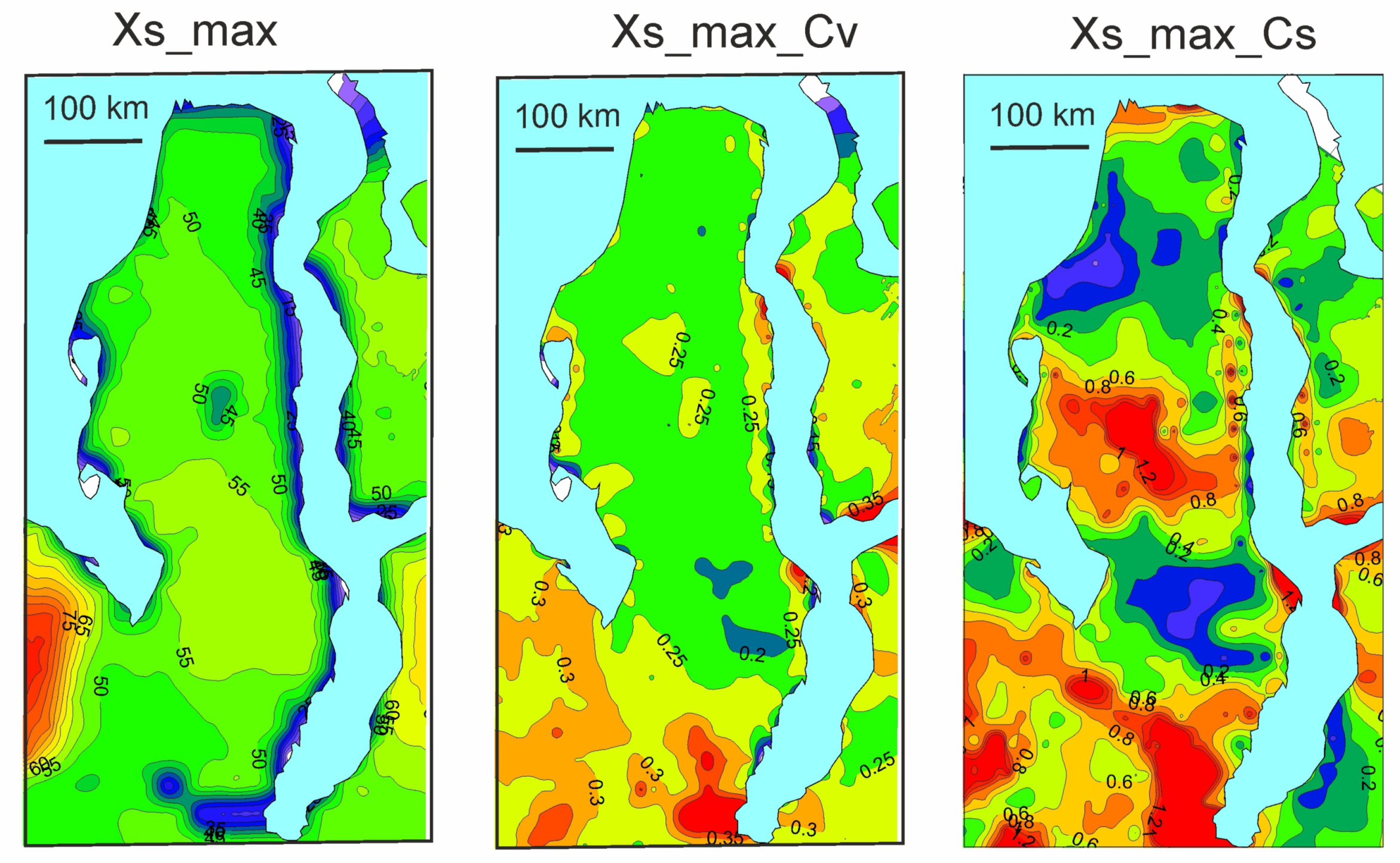
3.3.1. Mean Maximum Depth of Snow Cover and Surface Runoff Depth during the Snow Thaw Period

The spatial distribution of mean H_s (Figure 20) is rather uniform, with the maximum value of 210 mm of water equivalent in the central Yamal peninsula, and with the general trend to decrease both to the south and to the north. The bands of low values of H_s along the shores of the Ob Gulf and of the Kara Sea, as well as around large lakes, are artefacts of all reanalyses, where H_s values are taken equal to zero in the open water (see Table S1). These bands were excluded from further analysis.

The maximum depths of snow pack at the end of winter at meteorological stations on the Yamal peninsula, as well as maximum water content in snow in reanalysis data, are characterized by temporal trends (Figure 21). For the entire central Yamal there is no significant trend; linear regression coefficient for 35 years shows min-max deviations only ±5–10 cm around the mean; Student’s p-values for ERA5 data are over 20%. In the southern part of the peninsula this trend, if linear, is statistically significant, according to Student’s test with p-values less than 5%. This trend is pronounced only for the years 2014–2019, therefore these years were excluded in the analysis of calculated runoff characteristics during snow thaw period for all ERA5 nodes, so that temporal variability C_v and skewness C_s were calculated only for annual sequences without trend.

C_v changes are within 0.1–0.2 except for the areas south of the Baidaratskaya Bay. C_s spatial pattern is more complicated: four bands of high and low skewness values are alternating in latitudinal direction, showing probability distributions of H_s from highly asymmetrical to nearly symmetrical normal functions.

In this respect, the model is conservative–the total runoff during the snow thaw period X_sa is equal to the water equivalent in snow at the beginning of thaw period H_s plus precipitation P and minus evaporation E during this period. Therefore, the spatial distribution of mean annual runoff during the snow thaw period X_sa and its statistical characteristics are similar to those of H_s (Figure 22). Mean annual X_sa spatial pattern is rather uniform, with the maximum value of 250 mm at the central Yamal, with a general trend to decrease both to the south and to the north. C_v changes within 0.1–0.15 except of the areas south of the Baidaratskaya Bay. The skewness is close to zero, changing in the range −0.5~0.5 and showing nearly symmetrical normal distributions of X_sa.

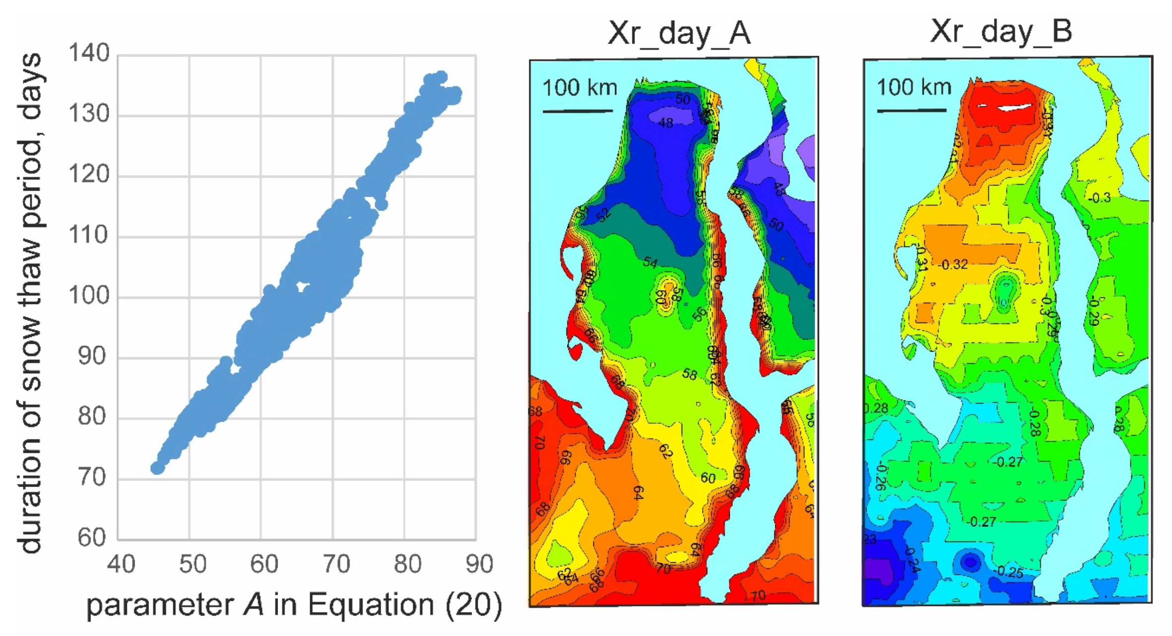
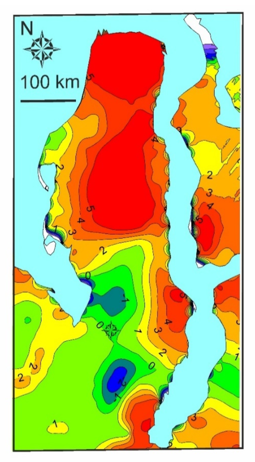
3.3.2. Daily Surface Runoff Depth During the Snow Thaw Period

The spatial pattern of annual maximum of daily surface runoff X_{s_max} and its statistics are in general similar to those of mean annual values (Figure 23). The pattern is also rather uniform, with the maximum value of 50–55 mm in the central Yamal peninsula, and with a general trend to decrease both to the south and to the north. Temporal variability of X_{s_max} is nearly the same for the entire Yamal peninsula, and C_v changes within 0.2–0.25, except for the areas south of the Baidaratskaya Bay. The spatial pattern of skewness is more complicated. 5–6 bands of high and low C_s values are alternating in the south-north direction, showing probability distributions of X_{s_max} from highly asymmetrical to nearly symmetrical one.

As mentioned above, the frequency-magnitude function, which describes the duration F of daily runoff depth ≥ X_d, is well approximated with Equation (20). The parameter A reflects the duration of snow thaw period, and parameter B shows the rate of exponential decrease of X_s duration.

Parameter A varies in the range 15–17 days in the central part of the Yamal peninsula and decreases to less than 10 days in the southern part of the territory. Parameter B varies from −0.05 to −0.08 on the entire Yamal peninsula (Figure 24).

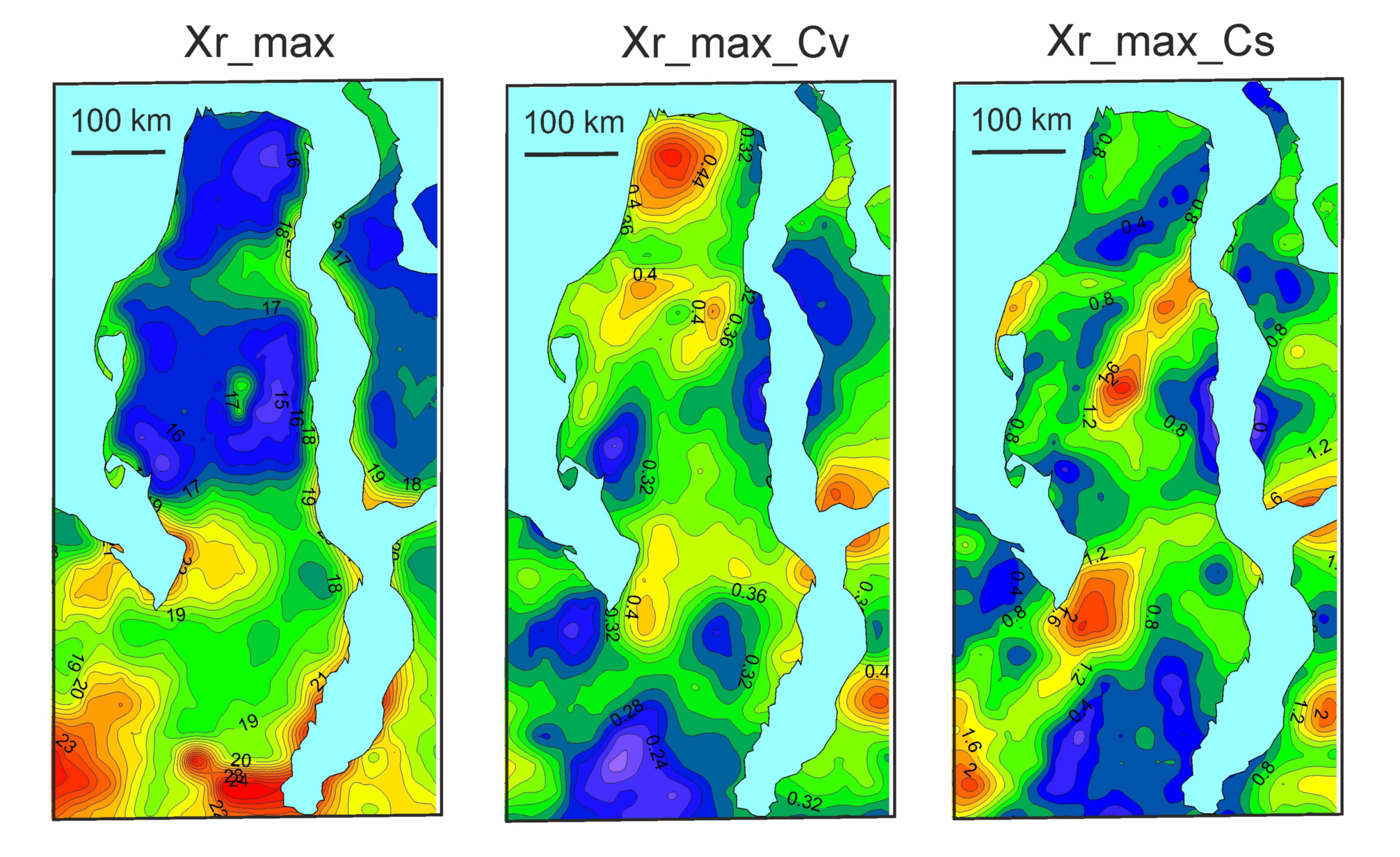
3.3.3. Mean Surface Runoff Depth of the Summer Rain Period

The temporal trends of mean surface runoff depth during the summer rains X_ra are not significant (Student’s p is more than 20% for all nodes of ERA-5) for both periods under investigations 1985–2019 and 1985–2013; the latter period is used further. X_ra decreases from south to north of the Yamal peninsula from 250 to 120 mm, and variability of its values (C_v) in general increases in the same direction from 0.2 to 0.3 (Figure 25). The skewness shows more complicated spatial pattern. Four latitudinal bands of high and low C_s values alternate in the north-south direction, showing probability distributions of annual surface runoff X_r from highly asymmetrical to nearly symmetrical.

The statistical characteristics of daily maximum of surface runoff X_{r_max} for the period of summer rains show in general the same spatial pattern. The mean maximum decreases from south to north from 24 to 15 mm. Variability of this maximum is greater than that of the mean X_ra values, increasing in the same direction from 0.24 to 0.5 (Figure 26). The skewness also shows four alternating bands of high and low C_s values.

The duration of daily surface runoff during summer rains follows Equation (20). Parameter A in Equation (20) reflects the duration of the period of summer rains, which is about 1.5 times longer than A (Figure 27). It decreases from 70 days in the southern part of the territory to 48 days at the northern part. Parameter B shows the rate of exponential decrease of daily X_r duration. The module of parameter B increases from south to north from 0.25 to 0.35 (Figure 27).

4. Discussion

The discussion should focus on the following key issues concerning the use of ERA5 for regional hydrological calculations: (a) statistical characteristics of the sequences with the trends; (b) the types of probability density functions used for different characteristics of surface runoff; (c) the effects of deviations of ERA5 data from the measured values on the results of runoff calculation with the hydrological model.

4.1. Statistical Characteristics of the Sequences with the Trends

Although the paper is devoted to regional studies, the problem of estimating statistical characteristics of hydrological sequences with pronounced trends is more general. A generally accepted assumption in hydrology is that mean values of data series and the first statistical moments are stable in time. This hypothesis, used at least during 20th century, becomes inapplicable now due to global climate changes. The mean global temperature is rapidly increasing, and the attempts of world community to slow down this rise are not effective yet. World hydrologic budget follows this trend, and global water resources must be recalculated in this new situation using existing models [52,53,54,55]. This is also true for any regional hydrological budgets [56,57,58], especially for the regions highly sensitive to temperature increase, such as the Arctic, now [59] and in the distant past [60]. On the Yamal peninsula, the recent stage of warming began somewhere between 1965 and the 1970s [36] and is evident in all climatic characteristics, of which air temperature for spring period, the maximum snow depth, water content in snow at the end of winter, and summer precipitation are of the main interest for the calculation of hydrologic sequences.

In this paper, we use a new assumption for the description of temporal sequences of hydrologic data: while the annual means or extremes of surface runoff change through time, the first two moments—dispersion and skewness—are statistically stable. The situation becomes even more complicated when there are long (multidecadal) waves in the changes of meteorological parameters against the background of the general linear trend for the entire period covered. For example, the snow pack depth at the end of the cold period at Novy Port station for the years 1940–2016 can be approximated with a linear trend. In this case, de-trended sequence shows a variability of C_v and of skewness C_s averaged with moving 10-year intervals, is subjected to longwave temporal changes (Figure 28). Then, for different time intervals, linear trends are different.

The temporal changes of input meteorological data in ERA5 and calculated hydrologic characteristics of the Yamal peninsula reveal not only a linear trend, but also long waves of temporal oscillations with periods of a decade to a few decades. The input data for the period of averaging at different sites can therefore contain a positive or negative linear trend or have no significant trend at all. This situation is typical for the distribution of the maximum snow pack depth on the Yamal peninsula. The time sequences of this characteristic during the years 1985–2019 at the south of peninsula show a statistically significant positive linear trend, according to Student’s test, with p-values less than 5%. This trend is still better described by non-linear functions. In this case, for the period 1985–2013 the trend becomes negligible and all increase in snow pack depth occurs only in the years 2014–2019 (see Figure 22). At the central and northern parts of the Yamal peninsula the linear temporal trend in snow pack depth is also negligible for the years 1985–2019, but it is negative and significant according to Student’s test with p-values less than 5% for the years 1985–2013. The analysis of trend influence on statistical moments is described in Appendix A. Variability of detrended sequences during the years 1985–2013 is lowest, therefore the statistics in Results, Section 3.3., and in Table S1 in Supplement were described for this very period.

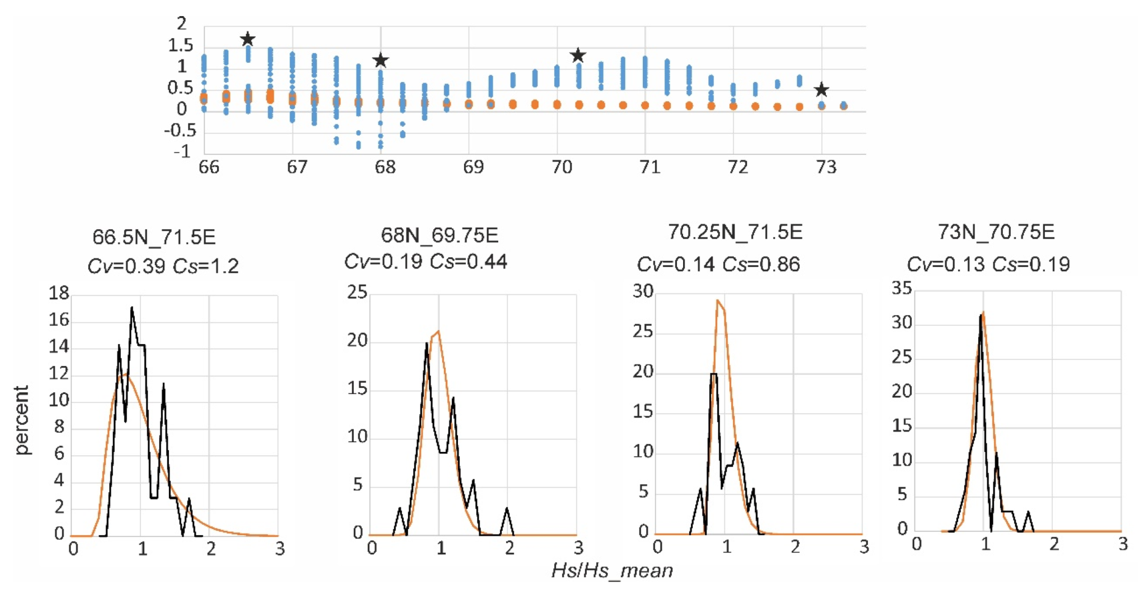
4.2. Types of Probability Density Functions Used for Different Characteristics of Surface Runoff

The second problem is also general, although it has specific features in different regions. The de-trended temporal sequences of annual means and maximums should be described by some probability density functions. In hydrology, Pearson’s type III distribution is often used for these purposes [61].

$$p\left(x\right)=\frac{1}{\beta \mathsf{\Gamma }\left(p\right)}{\left(\frac{x-\alpha }{\beta }\right)}^{p-1}exp\left(-\frac{x-\alpha }{\beta }\right)$$

(21)

Here x is a variable divided by its mean, $p={\left(\frac{2}{C_s}\right)}^2; \alpha =1-\frac{2C_v}{C_s}; \beta =\frac{C_v{C}_s}{2}$; Γ is gamma function. In this three-parameter function, skewness is usually estimated with a greater error than variance. Therefore, Equation (21) is usually transformed into two-parameter gamma-distribution (see Equation (18)), where C_s = 2C_v. For the Yamal peninsula over 80% of empirical distributions of annual snow pack depth fit this ratio within only 20% confident intervals for C_v and C_s. The spatial distribution of the C_s/C_v ratio demonstrates a regular pattern with high values of this ratio in the northern and central parts of the peninsula (very positively asymmetric functions) and with low values characteristic of the gamma function with median asymmetry and for the normal distribution (Figure 29). Distributions with skewness less than 0.17 should be described with other types of probability distribution functions, but such C_s values are rare. The main types of curves described with Equation (21) within Cv-Cs box, characteristic for Yamal, are shown in Figure 30.

Spatial distributions of C_s/C_v ratios for the sequences of mean and maximum surface runoff during the snow thaw period are in general similar to those of annual maximum snow pack depth H_s (see Figure 29), with greater spatial variability of this ratio.

The second important probability distribution function describes the duration F in days of daily runoff depth ≥ X (Equation (20))

$$F=Aexp\left(-BX\right)$$

(22)

Equation (22) is the simplified version of Gudrich distribution, commonly used for daily river runoff duration [62]

$$P={10}^{-c{Y}^n};Y=\frac{X_d-X_{d\_min}}{X_{d\_max}-X_{d\_min}}$$

(23)

When minimal daily runoff X_{d_min} is negligibly small and parameter n = 1, Equation (23) is similar to Equation (22).

Equation (22) by normalization and differentiation can be transformed into probability density function of daily surface runoff depth

$$\frac{dF}{dX}=\frac{d}{dX}\left(1-exp\left(-BX\right)\right)=Bexp\left(-BX\right)$$

(24)

Equation (24) is used in the application to calculate the volume of gully erosion with the model of gully potential estimations [10].

4.3. Effects of Errors in ERA5 Data on the Results of Runoff Calculations

The third problem to discuss is the applicability of ERA5 data for estimation of regional surface runoff with the use of the hydrological model. The main input meteorological data, used in the hydrological model, are air temperature, maximum depth of snow pack at the end of the cold period, and rainfall during the summer. The deviations of these ERA5 characteristics from the values measured at meteorological stations (Section 3.1) should be compared with the sensitivity of the hydrological model (Section 3.2). The response of the hydrological model to deviations in input values is nonlinear, therefore positive and negative deviations of measured values equal in module cause different deviations in calculated hydrological characteristics. Therefore, the mean differences in measured at seven meteorological stations and ERA5 values (“Error” in

Table 2. Sensitivity of the hydrological model to the errors in ERA5 data.

Meteorological Characteristic, Daily Mean	Error in ERA5	Hydrological Model Sensitivity
		Xd_max,		A		B
		Aer (mm)	Rer, %	Aer, Days	Rer (%)	Aer (mm)	Rer (%)
Air temperature during snow thaw period, °C	0.8/−0.6	−2/+7	−4/+14	1/−2	4/−11	−0.005/0.008	−9/14
Air temperature during the summer, °C	1.3/−0.9	+0.3/−9	+2/−6	11/−9	13/−11	0/−0.003	0/−0.8
Maximum depth of snow pack (water equivalent), mm	30/−60	+4.4/8.8	+10/−20	2/−5	9/−26	0.013/−0.035	13/−36
Rainfall during the summer, mm	2.6/−1.6	0.12/−0.1	0.6/−0.4	<±1	0.7/−0.5	0.002/−0.001	0.6/−0.4

An error is: (measured value) minus (value at ERA-5) (mean for 7 stations, separately for positive and negative errors); absolute model error Aer = (calculated value for input with +Error/−Error) minus (calculated value for input with zero Error); relative model error Rer = 100 × Aer/(value at zero Error).

) were calculated separately for positive and negative errors. The influence of these errors on the hydrological characteristics is important not only for surface runoff analysis but for further applications of surface runoff data. For example, for gully erosion modelling [10] the most important hydrological characteristics are the maximum of daily surface runoff for the periods of snow thaw and summer rains Xd_max and parameters A and B in daily runoff duration function (Equation (20)).

As can be seen from Table 2, air temperature error within the range 1.4~2.2 °C significantly influences Xd_max in the range of 18% for the spring and 8% for the summer. As the estimates of gully erosion potential are directly related to the absolute values of Xd_max, this error must be taken into account in the analysis of erosion characteristics. The same is true for the error of maximum depth of snow pack, which causes error in the calculations of extreme surface runoff during the snow thaw within 30%.

5. Conclusions

The annual and extreme surface runoff characteristics (means, first two statistical moments, and probability distribution functions) were calculated for the entire Yamal peninsula. For these purposes we developed the hydrological model of surface runoff estimation. Two main sources of water are typical for this environment: snow thaw during the spring and rainfall during the summer. In the conditions of Arctic climate with deep permafrost, the losses in runoff are limited to evaporation, as soil permeability is negligible. The model was calibrated on the available measurements. The meteorological base for hydrological calculations was ERA5 reanalysis. The reanalysis data were validated on the available meteorological measurements for this region and showed air temperature error 0.8/−0.6 °C, maximum depth of snow pack (water equivalent) error 30/−60 mm, and rainfall during the summer error 2.6/−1.6 mm. These deviations of reanalysis data from the measurements cause the errors in the results of surface runoff calculation, mainly within the snow thaw period. The daily surface runoff, its maximum value, and parameters of distribution functions surface runoff duration, vary in the range 18–30% due to ERA5 errors in air temperature and snow cover depth. As the characteristics of daily surface runoff are the main input to the models of gully erosion, these errors should be taken into account in the further modelling of gully erosion processes on the Yamal peninsula.

References

1. Dobrinski, L.N. (Ed.) Nature of Yamal (Priroda Yamala); Nauka: Ekaterinburg, Russia, 1995; p. 435. (In Russian) [Google Scholar]
2. Litvinenko, V. The Role of Hydrocarbons in the Global Energy Agenda: The Focus on Liquefied Natural Gas. Resources 2020, 9, 59. [Google Scholar] [CrossRef]
3. Paltsev, S. Scenarios for Russia’s natural gas exports to 2050. Energy Econ. 2014, 42, 262–270. [Google Scholar] [CrossRef]
4. Henderson, J.; Yermakov, V. Russian LNG: Becoming a Global Force. Working Paper; Oxford Institute for Energy Studies: Oxford, UK, 2019; p. 37. [Google Scholar]
5. IGU. Global Gas Report 2019; International Gas Union: Barcelona, Spain, 2020. Available online: https://media-publications.bcg.com/SNAM-2019-GGR.pdf (accessed on 6 June 2020).
6. IGU. World LNG Report 2020; International Gas Union: Barcelona, Spain, 2020. Available online: https://www.igu.org/sites/default/files/node-document-field_file/2020%20World%20LNG%20Report.pdf (accessed on 6 June 2020).
7. Novikov, S.M. Hydrology of the Wetlands of the Permafrost Zone of Western Siberia (Gidrologiya Zabolochennykh Territoriy Zony Mnogoletney Merzloty Zapadnoy Sibiri); VVM Publicaiton House: St. Petersburg, Russia, 2009; p. 536. (In Russian) [Google Scholar]
8. Bobrovitskaya, N.N.; Baranov, A.V.; Vasilenko, N.N.; Zubkova, K.M. Hydrological Conditions. In Erosion Processes at the Central Yamal (Erozionnyye Protsessy Tsentral’Nogo Yamala); Sidorchuk, A., Baranov, A., Eds.; RNII KPN: St. Petersburg, Russia, 1999; pp. 90–105. (In Russian) [Google Scholar]
9. Sidorchuk, A. Gully erosion in the cold environment: Risks and hazards. Adv. Environ. Res. 2015, 44, 139–192. [Google Scholar]
10. Sidorchuk, A. The potential of gully erosion on the Yamal peninsula, West Siberia. Sustainability 2020, 12, 260. [Google Scholar] [CrossRef] [Green Version]
11. Patton, P.C.; Schumm, S.A. Gully erosion, northwestern Colorado: A threshold phenomenon. Geology 1975, 3, 83–90. [Google Scholar] [CrossRef]
12. Vandaele, K.; Poesen, J.; Govers, G.; van Wesemael, B. Geomorphic threshold conditions for ephemeral gully incision. Geomorphology 1996, 16, 161–173. [Google Scholar] [CrossRef]
13. Garrett, K.K.; Wohl, E.E. Climate-invariant area–slope relations in channel heads initiated by surface runoff. Earth Surf. Process. Landforms 2017, 42, 1745–1751. [Google Scholar] [CrossRef]
14. Sidorchuk, A. Dynamic and static models of gully erosion. Catena 1999, 37, 401–414. [Google Scholar] [CrossRef]
15. Sagintayev, Z.; Sultan, M.; Khan, S.D.; Khan, S.A.; Mahmood, K.; Yan, E.; Milewski, A.; Marsala, P. A remote sensing contribution to hydrologic modelling in arid and inaccessible watersheds, Pishin Lora basin, Pakistan. Hydrol. Process. 2012, 26, 85–99. [Google Scholar] [CrossRef]
16. Cole, S.J.; Moore, R.J. Distributed hydrological modelling using weather radar in gauged and ungauged basins. Adv. Water Resour. 2009, 32, 1107–1120. [Google Scholar] [CrossRef] [Green Version]
17. Lindsay, R.; Wensnahan, M.; Schweiger, A.; Zhang, J. Evaluation of seven different atmospheric reanalysis products in the Arctic. J. Clim. 2014, 27, 2588–2606. [Google Scholar] [CrossRef] [Green Version]
18. Liu, Z.; Liu, Y.; Wang, S.; Yang, X.; Wang, L.; Baig, M.H.A.; Chi, W.; Wang, Z. Evaluation of spatial and temporal performances of ERA-Interim precipitation and temperature in mainland China. J. Clim. 2018, 31, 4347–4365. [Google Scholar] [CrossRef]
19. Lader, R.; Bhatt, U.S.; Walsh, J.E.; Rupp, T.S.; Bieniek, P.A. Two-meter temperature and precipitation from atmospheric reanalysis evaluated for Alaska. J. Appl. Meteorol. Climatol. 2016, 55, 901–922. [Google Scholar] [CrossRef]
20. Timmermans, B.; Wehner, M.; Cooley, D.; O’Brien, T.; Krishnan, H. An evaluation of the consistency of extremes in gridded precipitation data sets. Clim. Dyn. 2019, 52, 6651–6670. [Google Scholar] [CrossRef] [Green Version]
21. Albergel, C.; Munier, S.; Bocher, A.; Bonan, B.; Zheng, Y.; Draper, C.; Leroux, D.J.; Calvet, J.-C. LDAS-Monde Sequential Assimilation of Satellite Derived Observations Applied to the Contiguous US: An ERA5 Driven Reanalysis of the Land Surface Variables. Remote Sens. 2018, 10, 1627. [Google Scholar] [CrossRef] [Green Version]
22. Gampe, D.; Ludwig, R. Evaluation of gridded precipitation data products for hydrological applications in complex topography. Hydrology 2017, 4, 53. [Google Scholar] [CrossRef] [Green Version]
23. Essou, G.R.; Brissette, F.; Lucas-Picher, P. The use of reanalyses and gridded observations as weather input data for a hydrological model: Comparison of performances of simulated river flows based on the density of weather stations. J. Hydrometeorol. 2017, 18, 497–513. [Google Scholar] [CrossRef]
24. Raimonet, M.; Oudin, L.; Thieu, V.; Silvestre, M.; Vautard, R.; Rabouille, C.; Le Moigne, P. Evaluation of gridded meteorological datasets for hydrological modelling. J. Hydrometeorol. 2017, 18, 3027–3041. [Google Scholar] [CrossRef]
25. Beck, H.E.; Vergopolan, N.; Pan, M.; Levizzani, V.; Van Dijk, A.I.; Weedon, G.P.; Brocca, L.; Pappenberger, F.; Huffman, G.J.; Wood, E.F. Global-Scale Evaluation of 22 Precipitation Datasets Using Gauge Observations and Hydrological Modelling. In Satellite Precipitation Measurement; Springer: Cham, Switzerland, 2020; pp. 625–653. [Google Scholar]
26. Mahto, S.S.; Mishra, V. Does ERA-5 outperform other reanalysis products for hydrologic applications in India? J. Geophys. Res. Atmos. 2019, 124, 9423–9441. [Google Scholar] [CrossRef]
27. Nkiaka, E.; Nawaz, N.R.; Lovett, J.C. Evaluating global reanalysis datasets as input for hydrological modelling in the Sudano-Sahel region. Hydrology 2017, 4, 13. [Google Scholar] [CrossRef] [Green Version]
28. Fuka, D.R.; Walter, M.T.; MacAlister, C.; Degaetano, A.T.; Steenhuis, T.S.; Easton, Z.M. Using the Climate Forecast System Reanalysis as weather input data for watershed models. Hydrol. Process. 2014, 28, 5613–5623. [Google Scholar] [CrossRef]
29. Essou, G.R.; Sabarly, F.; Lucas-Picher, P.; Brissette, F.; Poulin, A. Can precipitation and temperature from meteorological reanalyses be used for hydrological modelling? J. Hydrometeorol. 2016, 17, 1929–1950. [Google Scholar] [CrossRef]
30. Ayzel, G.; Varentsova, N.; Erina, O.; Sokolov, D.; Kurochkina, L.; Moreydo, V. OpenForecast: The First Open-Source Operational Runoff Forecasting System in Russia. Water 2019, 11, 1546. [Google Scholar] [CrossRef] [Green Version]
31. Lauri, H.; Räsänen, T.A.; Kummu, M. Using reanalysis and remotely sensed temperature and precipitation data for hydrological modelling in monsoon climate: Mekong River case study. J. Hydrometeorol. 2014, 15, 1532–1545. [Google Scholar] [CrossRef]
32. Nguyen, T.H.; Masih, I.; Mohamed, Y.A.; Van der Zaag, P. Validating Rainfall-Runoff Modelling Using Satellite-Based and Reanalysis Precipitation Products in the Sre Pok Catchment, the Mekong River Basin. Geosciences 2018, 8, 164. [Google Scholar] [CrossRef] [Green Version]
33. Krogh, S.A.; Pomeroy, J.W.; McPhee, J. Physically based mountain hydrological modelling using reanalysis data in Patagonia. J. Hydrometeorol. 2015, 16, 172–193. [Google Scholar] [CrossRef] [Green Version]
34. Jing, W.; Song, J.; Zhao, X. Validation of ECMWF Multi-Layer Reanalysis Soil Moisture Based on the OzNet Hydrology Network. Water 2018, 10, 1123. [Google Scholar] [CrossRef] [Green Version]
35. Kottek, M.; Grieser, J.; Beck, C.; Rudolf, B.; Rubel, F. World map of the Köppen-Geiger climate classification updated. Meteorol. Z. 2006, 15, 259–263. [Google Scholar] [CrossRef]
36. Vikhamar-Schuler, D.; Hanssen-Bauer, I.; Førland, E.J. Long-Term Climate Trends of the Yamalo-Nenets AO, Russia; Norwegian Meteorological Institute: Oslo, Norway, 2010; pp. 1–51. [Google Scholar]
37. Bulygina, O.N.; Veselov, V.M.; Razuvaev, V.N.; Aleksandrova, T.M. Description of the Dataset of Observational Data on Major Meteorological Parameters from Russian Weather Stations. Database State Registration Certificate No. 1 49 2014. Available online: http://meteo.ru/data (accessed on 12 June 2020). (In Russian).
38. Vasiliev, A.A.; Gravis, A.G.; Gubarkov, A.A.; Drozdov, D.S.; Korostelev, Y.V.; Malkova, G.V.; Oblogov, G.E.; Ponomareva, O.E.; Sadurtdinov, M.R.; Streletskaya, I.D.; et al. Permafrost degradation: Results of the long-term geocryological monitoring in the western sector of Russian Arctic. Kriosf. Zemli 2020, 24, 15–30. (In Russian) [Google Scholar] [CrossRef]
39. Borodulin, V.V.; Gryazeva, L.I. The results of hydrological studies of the Yamal rivers. Meteorol. Hydrol. 1993, 3, 86–94. (In Russian) [Google Scholar]
40. Sidorchuk, A. Gully Thermoerosion on the Yamal Peninsula. In Geomorphic Hazards; Slaymaker, O., Ed.; Wiley: Chichester, UK, 1996; pp. 141–153. [Google Scholar]
41. Hersbach, H.; Dee, D. ERA5 reanalysis is in production. ECMWF Newsl. 2016, 147, 7. [Google Scholar]
42. Rango, A.; Martinec, J. Revisiting the Degree-day Method for Snowmelt Computations. J. Am. Water Resour. Assoc. 2007, 31, 657–669. [Google Scholar] [CrossRef]
43. Pistocchi, A.; Bagli, S.; Callegari, M.; Notarnicola, C.; Mazzoli, P. On the Direct Calculation of Snow Water Balances Using Snow Cover Information. Water 2017, 9, 848. [Google Scholar] [CrossRef] [Green Version]
44. Komarov, V.D.; Makarova, T.T.; Sinegub, E.S. Calculation of the hydrograph of floods of small lowland rivers based on thaw intensity data. Proc. Hydrometeorol. Cent. USSR 1969, 37, 3–30. (In Russian) [Google Scholar]
45. Vinogradov, Y.B. Mathematical Modelling of Flow Formation Processes (Matematicheskoye Modelirovaniye Protsessov Formirovaniya Stoka); Gidrometeoizdat: Leningrad, Russia, 1988; p. 312. (In Russian) [Google Scholar]
46. Vinogradov, Y.B.; Vinogradova, T.A.; Zhuravlev, S.A.; Zhuravleva, A.D. Mathematical modelling of hydrographs from the unstudied river basins on the Yamal peninsula. Bull. St. Petersburg State Univ. 2014, 7, 71–81. (In Russian) [Google Scholar]
47. Gelfan, A.N. Model of Formation of River Flow during Snowmelt and Rain. In Erosion Processes at the Central Yamal (Erozionnyye Protsessy Tsentral’Nogo Yamala); Sidorchuk, A., Baranov, A., Eds.; RNII KPN: St. Petersburg, Russia, 1999; pp. 205–225. (In Russian) [Google Scholar]
48. Popov, Y.G. Analysis of River Flow Formation (Analiz Formirovaniya Stoka Ravninnykh Rek); Gidrometeoizdat: Leningrad, Russia, 1956; p. 131. (In Russian) [Google Scholar]
49. Bosilovich, M.L.G.; Chen, J.; Robertson, F.R.; Adler, R.F. Evaluation of global precipitation in reanalyses. J. Appl. Meteorol. Climatol. 2008, 47, 2279–2299. [Google Scholar] [CrossRef]
50. Donat, M.G.; Sillmann, J.; Wild, S.; Alexander, L.V.; Lippmann, T.; Zwiers, F.W. Consistency of temperature and precipitation extremes across various global gridded in situ and reanalysis datasets. J. Clim. 2014, 27, 5019–5035. [Google Scholar] [CrossRef]
51. Recalculation of Coordinates. Available online: https://geobridge.ru/proj#null (accessed on 12 May 2020).
52. Sood, A.; Smakhtin, V. Global hydrological models: A review. Hydrol. Sci. J. 2015, 60, 549–565. [Google Scholar] [CrossRef]
53. Her, Y.; Yoo, S.; Cho, J.; Hwang, S.; Jeong, J.; Seong, C. Uncertainty in hydrological analysis of climate change: Multi-parameter vs. multi-GCM ensemble predictions. Sci. Rep. 2019, 9, 4974. [Google Scholar] [CrossRef] [Green Version]
54. Gleick, P.H. Water in Crisis: A Guide to the World’s Fresh Water Resources; Oxford University Press: Oxford, UK, 1993; p. 473. [Google Scholar]
55. Hurlimann, A.; Wilson, E. Sustainable Urban Water Management under a Changing Climate: The Role of Spatial Planning. Water 2018, 10, 546. [Google Scholar] [CrossRef] [Green Version]
56. Versini, P.-A.; Pouget, L.; Mcennis, S.; Custodio, E.; Escaler, I. Climate change impact on water resources availability—Case study of the Llobregat River basin (Spain). Hydrol. Sci. J. 2016, 61, 2496–2508. [Google Scholar] [CrossRef]
57. Bodian, A.; Diop, L.; Panthou, G.; Dacosta, H.; Deme, A.; Dezetter, A.; Ndiaye, P.M.; Diouf, I.; Vischel, T. Recent Trend in Hydroclimatic Conditions in the Senegal River Basin. Water 2020, 12, 436. [Google Scholar] [CrossRef] [Green Version]
58. Deng, W.; Song, J.; Bai, H.; He, Y.; Yu, M.; Wang, H.; Cheng, D. Analyzing the Impacts of Climate Variability and Land Surface Changes on the Annual Water–Energy Balance in the Weihe River Basin of China. Water 2018, 10, 1792. [Google Scholar] [CrossRef] [Green Version]
59. Krogh, S.A.; Pomeroy, J.W. Impact of future climate and vegetation on the hydrology of an Arctic headwater basin at the tundra–taiga transition. J. Hydrometeorol. 2019, 20, 197–215. [Google Scholar] [CrossRef]
60. Sidorchuk, A.Y.; Matveeva, T.A. Periglacial gully erosion on the east European plain and its recent analog at the Yamal peninsula. Geogr. Environ. Sustain. 2020, 13, 183–194. [Google Scholar] [CrossRef] [Green Version]
61. Thompson, S.A. Hydrology for Water Management, 1st ed.; Balkema Publication: Rotterdam, The Netherlands, 1999; p. 380. [Google Scholar]
62. Meylan, P.; Favre, A.-C.; Musy, A. Predictive Hydrology: A Frequency Analysis Approach; Taylor & Francis Inc.: Abingdon, UK, 2012; p. 212. [Google Scholar]
Figure 1. The Yamal peninsula.
Water 12 02099 g001
Figure 2. Mean surface (2 m) air temperature (°C) (a,c) and linear trend (per decade) (b,d) in January (top) and in July (bottom) based on ERA5 Reanalysis for 1985–2019.
Water 12 02099 g002
Figure 3. Averaged seasonal cycle of surface air temperature (2 m) for four meteorological stations.
Water 12 02099 g003
Figure 4. Meteorological stations (red dots) and nearest to them ERA5 reanalysis grid points (blue dots) used in the study. The black squares show the position of State Hydrological Institute measurements in 1985–1997, the star shows the position of State Hydrological Institute and Moscow State University measurements in 1990–1993.
Water 12 02099 g004
Figure 5. The block-diagram of the surface runoff calculation with the melt coefficient approach.
Water 12 02099 g005
Figure 6. The comparison of the surface runoff depth calculated with the model, taking the melt coefficient ksm = 1.25 × 10⁻⁴ and measured daily runoff depth Xs (mm) during snow thaw periods of the years 1992 and 1993 (a) at the headwaters of the Anthropogenic gully on the Yamal peninsula (b). The lower figures show the calculated (blue lines) and measured (red lines) hydrographs for the years 1992 (c) and 1993 (d).
Water 12 02099 g006
Figure 7. 2m air temperature at seven stations (red) and at the nearest grid points of ERA5 reanalysis (blue) for the periods of snow thaw (a) and summer rains (b). Boxes indicate the lower and upper quartile. Horizontal line in each box represents the median t2m air temperature. “Whiskers” extending from each box represent the minimum and maximum temperature recorded for each station.
Water 12 02099 g007
Figure 8. Error statistics (ERA5 versus observational data) for daily t2m: root mean square error (RMSE) (a), correlation coefficient (b), the ratio of the standard deviations (STD) of the ERA5 reanalysis and observed values (c) for seven stations and the nearest grid points of ERA5 reanalysis for snow thaw (orange) and summer rains (green) periods.
Water 12 02099 g008
Figure 9. Whisker-box plot (left column) and 95th percentile (right column) of total daily precipitation for seven stations (red) and the nearest grid points of ERA5 reanalysis (blue) for cold (a,b), snow thaw (c,d) and summer rains (e,f) periods. Boxes indicate the lower and upper quartile. Horizontal line in each box represents the median t2m air temperature. Vertical lines extending from each box represent the minimum and maximum temperature recorded for that station.
Water 12 02099 g009
Figure 10. Error statistics (ERA5 versus observational data) for total daily precipitation: root mean square error (RMSE) (a), correlation coefficient (b), the ratio of the standard deviations (STD) of the ERA5 reanalysis and observed values (c) for seven stations and the nearest grid points of ERA5 reanalysis for cold (blue), snow thaw (orange) and summer rains (green) periods.
Water 12 02099 g010
Figure 11. Whisker-box plot of maximum snow height at the end of cold season for seven stations (red) and the nearest grid points of ERA5 reanalysis (blue) (a) and RMSE for maximum snow height for seven stations and the nearest grid points of ERA5 reanalysis (b). Boxes in (a) indicate the lower and upper quartile. Horizontal line in each box represents the median t2m air temperature. Vertical lines extending from each box represent the minimum and maximum temperature recorded for that station.
Water 12 02099 g011
Figure 12. Mean date of maximum snow height at the end of cold season (a) and RMSE (b) for seven stations and the nearest grid points of ERA5 reanalysis.
Water 12 02099 g012
Figure 13. Effect of variability of total surface runoff Xsa during snow thaw period on the variability of the maximum daily runoff Xs_max.
Water 12 02099 g013
Figure 14. Effect of variability of maximum daily surface runoff Xs_max on the parameter A (a) and B (b) of the exponential changes in duration of daily runoff Xs (Equation (20)).
Water 12 02099 g014
Figure 15. Changes in shape of hydrograph of daily runoff during the snow thaw period with variations of daily air temperatures, an example for 1992 year.
Water 12 02099 g015
Figure 16. Changes in mean daily runoff maximum (triangles) and duration of the snow thaw period (circles) with variations of daily air temperatures.
Water 12 02099 g016
Figure 17. The differences in air temperature regimen during the snow thaw period and associated types of respond of timing of maximum Xs_max to an increase of ksm. For details, see the text.
Water 12 02099 g017
Figure 18. Changes in the duration of the warm period (triangles) and in the mean daily runoff maximum (circles) with variations of daily air temperatures.
Water 12 02099 g018
Figure 19. ERA5 grid and corresponding MSK-1964 coordinates (in km from datum) for the Yamal peninsula.
Water 12 02099 g019
Figure 20. Spatial distributions of mean annual Hs, its temporal variability Cv and skewness Cs. on the Yamal peninsula.
Water 12 02099 g020
Figure 21. Temporal changes of maximum snow pack depth at the end of the winter at the Novy Port station for two periods–1940–2016 and 1985–2016, and the same for the second mentioned interval from ERA5 reanalysis at the nearest grid node.
Water 12 02099 g021
Figure 22. Spatial distributions of mean annual Xsa and its temporal variability Cv and skewness Cs on the Yamal peninsula.
Water 12 02099 g022
Figure 23. Spatial distributions of mean annual maximum of daily surface runoff Xs_max for the period of snow thaw, its temporal variability Cv and skewness Cs on the Yamal peninsula.
Water 12 02099 g023
Figure 24. The relationship between parameter A and duration of snow show period (left) and spatial distributions of parameters A and B in Equation (20).
Water 12 02099 g024
Figure 25. Spatial distributions of mean surface runoff Xr, its temporal variability Cv and skewness Cs for the period of summer rains on the Yamal peninsula.
Water 12 02099 g025
Figure 26. Spatial distributions of daily maximum of surface runoff Xr_max, its temporal variability Cv and skewness Cs for the period of summer rains on the Yamal peninsula.
Water 12 02099 g026
Figure 27. The relationship between parameter A and duration of summer rains period (left) and spatial distributions of parameters A and B in Equation (20) on the Yamal peninsula.
Water 12 02099 g027
Figure 28. Characteristics of de-trended sequences of snow pack depth at the Novy Port station. See the text for the details.
Water 12 02099 g028
Figure 29. Spatial distribution of Cs/Cv ratios for sequences of annual maximum snow pack depth Hs during the years 1985–2013 with linear trend excluded.
Water 12 02099 g029
Figure 30. Probability density functions (PDF) for typical combinations of Cs and Cv of normalized annual maximum Hs: black line–PDF on measured data; red–PDF calculated with Equation (21). The upper figure shows the position (stars) of these combinations of Cs (blue dots) and Cv (red dots) along the south-north direction (from 66 to 73.5° N). The scatter shows change of the statistics in west-east direction.
Water 12 02099 g030