Development and Sensitivity Analysis of an Empirical Equation for Calculating the Amplitude of Pressure Head Loss of Oscillating Water Flow in Different Types of Pipe

Abstract

Low pressure oscillating water flow can reduce the investment and energy consumption of irrigation. It is also effective in reducing the clogging of an emitter and improving the spraying quality of sprinklers. In order to overcome the problem of the complex process in calculating the amplitude of the pressure head loss of oscillating water flow in different types of pipes, in this study, an empirical equation for the amplitude of the pressure head loss of oscillating water flow in different types of pipe has been developed. Further, validation experiments have been conducted to verify the accuracy of the calculated amplitudes of the pressure head loss by the empirical equation. The results show that average relative error between the measured and the calculated amplitudes of the pressure head loss by the empirical equation is 10.77%. Since the relative errors are small, it is an indication that the amplitudes of the pressure head loss calculated by the empirical equation are accurate. For the empirical equation developed in this study, the sensitivity of the model parameters has been analyzed. The results show that the amplitude of velocity, the internal pipe diameter, and the length of pipe are classified as highly sensitive. The average velocity, the period of oscillating water flow, and the modulus of elasticity of the pipe material are classified as sensitive. The thickness of the pipe wall is classified as medium sensitive. Compared with the calculation models of the existing researches, the empirical equation reduces the number of parameters required to be calculated, by which many complicated calculations are avoided, which greatly improves the computing efficiency. This is conducive to the efficient operation and management of oscillating water flow in irrigation pipe networks and also provides help for the optimal design of irrigation pipe networks.

1. Introduction

The considerable investment and cost of energy required for irrigation greatly challenges the wide application of irrigation. The main method to lower the operating and energy costs in irrigation is to reduce the operating pressure of irrigation. Irrigation with low operating pressure does not require high-power pumps or other high-standard water supply facilities. This is conducive to the wide application of irrigation in areas where water-supply facilities are inadequate and sparse [1,2,3,4,5,6]. Low-pressure drip irrigation uses lower water pressure, which produces slow water flow velocity in the emitter. Due to the slow flow velocity, it increases the probability of the suspended solids being deposited in the emitter passage, resulting in more clogging of the emitter [7,8,9,10]. Sprinkler irrigation under low pressure gives an uneven water distribution, excessive high sprinkler intensity in areas where the water distribution is concentrated, or excessive kinetic energy of water droplets. All of these result in soil erosion and surface runoff [11,12]. Currently, the common method to overcome these problems is to optimize the structures of the emitters and sprinklers. For example, the geometric parameters of the flow passage of the emitter are designed so as to alleviate clogging of the emitter under low operating pressure [13,14,15,16]. Furthermore, adding a water dispersing device, jet device, or other devices to the sprinklers can improve the uniformity of the water distribution under low operating pressure [17,18,19]. However, the optimization of such equipment structures requires time and capital investment, and the effects of the optimizations remain limited.

Traditional irrigation uses constant water pressure. However, in recent years, the applications of oscillating water flow with low operating pressure in irrigation showed that they can overcome the above-mentioned problems. The turbulence in the passage of emitter is more intense because of the oscillating water flow, thereby increasing the water flow velocity in the emitter, decreasing the probability of deposition of the suspended solids in the emitter passage, and reducing the clogging in the emitter [20,21,22]. Oscillating water flow can significantly improve the uniformity of the water distribution of sprinklers and reduce the high sprinkler intensity and kinetic energy of water droplets of sprinklers, thereby lessening soil erosion and surface runoff [23,24,25,26]. This application differs from common transient flow, such as water hammers in water conservancy engineering structures (e.g., hydropower stations and pump stations), where instantaneous pressure head changes irregularly over time. The research on water hammers is relatively mature, and many methods, such as the method of characteristics, have been developed, which can calculate the instantaneous pressure head [27,28,29,30,31,32]. On the other hand, the instantaneous pressure head of oscillating water flow changes periodically over time, and both the maximum and minimum instantaneous pressure heads remain basically the same, as shown in Figure 1. The variation law of the instantaneous discharge and instantaneous velocity of oscillating water flow with time is similar to that of instantaneous pressure head. However, the research on the instantaneous pressure head calculation of oscillation water flow has only just started, in which a complex function has been used to solve both the continuity equation and the momentum equation of transient flow. A model that can calculate the amplitude of the pressure head loss of oscillation water flow in a pipe accurately has been developed [33].

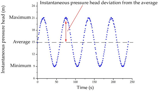
Figure 1. Instantaneous pressure head of oscillating water flow.

As mentioned above, the earlier research on oscillating water flow in irrigation focuses on improving the spraying quality of low-pressure sprinkler irrigation as well as the anti-clogging effect of emitters. After oscillating water flow is generated, it can only reach the sprinklers and emitters through a pipe. However, using the calculation models from the existing research to calculate the amplitude of the pressure head loss of oscillating water flow needs a computer to carry out many complicated calculations. In the absence of a computer, it is not convenient and efficient to calculate the amplitude of the pressure head loss using the existing calculation models. Hence, it is not efficient to use the existing calculation models to design and operate irrigation pipe networks. In addition, the earlier research shows that the existing calculation models only give high accuracy for flow in PVC (Polyvinyl chlorid) pipe.

Therefore, in order to overcome the problem of the complex calculation process of the amplitude of the pressure head loss of oscillating water flow in different types of pipe, in this study, Buckingham’s pi-theorem has been used to conduct a dimensional analysis of the physical parameters of oscillating water flow in a pipe. In addition, experiments of oscillating water flow in different types of pipe have been conducted. In order to develop an empirical equation for the amplitude of the pressure head loss of oscillating water flow in different types of pipe, the SPSS software (Statistical Product and Service Solutions) has been used for the regression analyses of the experimental data. In order to verify the accuracy of the empirical equation, validation experiments have been conducted. Finally, the sensitivity of the parameters of the empirical equation have been analyzed. The objective of this study is to develop an equation that can be used to calculate the amplitude of the pressure head loss of oscillating water flow in different types of pipe and for the design and operation of pipe networks.

2. Material and Methods

2.1. Experiments

2.1.1. Experimental Equipment and Procedure

As shown in Figure 2, the main components of the experimental equipment for testing the oscillating water flow are the pipes, water tank, pump, variable frequency drive, computer, pressure transducers (range = 0–0.6 MPa, accuracy = 0.1%), and electromagnetic flowmeter (range = 0.07–80 m3/h). The oscillating water flow is generated by a programmable logic controller (PLC), variable frequency drive, and pump. The program for the oscillating water flow mode is input into the programmable logic controller to control the variable frequency drive, which controls the operating frequency of the pressurized pump. When setting the oscillating water flow parameters, the maximum and minimum of instantaneous pressure heads can also be set, and the period of oscillating water flow can be adjusted. The pressure signal and discharge signal are recorded by a signal collector and sent to a computer.

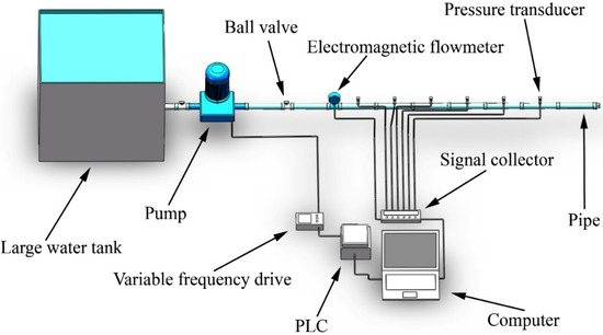
Figure 2. Experimental setup for testing oscillating water flow in a pipe.

2.1.2. Experimental Setup

In order to develop an empirical equation for the amplitude of the pressure head loss of different types of pipe, five pipes of different types have been used in the experiments. The modulus of elasticity of the five pipes are different. Figure 3 shows the five types of pipes. The pipe used in the experimental Cases C1-1 to C1-8 is PE (polyethylene) drip tape. The pipe used in the experimental Cases C2-1to C2-8 is ABS (acrylonitrile-butadiene-styrene) pipe. The pipe used in the experimental Cases C3-1to C3-8 is PVC (polyvinyl chloride) pipe. The pipe used in the experimental Cases C4-1 to C4-8 is PS (polystyrene) pipe. Finally, the pipe used in the experimental Cases C5-1 to C5-8 is PP (perspex) pipe. For the 40 experimental cases, the physical parameters of the oscillating water flow and the pipe are shown in Table 1. For each experimental case, pressure transducers have been installed along the 48 m long pipe at an interval of 8 m so as to measure the flow pressure at six different locations along the pipe. Therefore, for the 40 experimental cases, 240 pressure data points have been obtained.

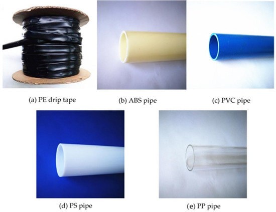
Figure 3. Five types of pipes used in the experiments.

Table 1. Physical parameters of oscillating water flow and pipe used in the experiments.

Case	${\overline{\mathbf{H}}}_1\left(\mathbf{m}\right)$	${\mathbf{h}}_1^{*}\left(\mathbf{m}\right)$	${\overline{\mathbf{V}}}_1$$(\mathbf{m}/\mathbf{s})$	${\mathbf{v}}_1^{*}$$(\mathbf{m}/\mathbf{s})$	P(s)	$\mathbf{E}({10}^9\mathbf{N}/{\mathbf{m}}^2)$	D(m)	$\mathsf{\delta }$	L(m)
C1-1	3.92	2.48	0.6	0.25	30	0.8	0.0274	0.0003	48
C1-2	5.17	3.36	0.72	0.35	43	0.8	0.0312	0.0004	48
C1-3	8.69	1.99	1.2	0.12	36	0.8	0.0392	0.0004	48
C1-4	7.67	5.2	1.18	0.6	55	0.8	0.047	0.0005	48
C1-5	10.21	4.49	1.48	0.5	70	0.8	0.049	0.0005	48
C1-6	11.76	4.86	1.68	0.5	78	0.8	0.0616	0.0007	48
C1-7	13.36	5.39	2.32	0.48	65	0.8	0.0734	0.0008	48
C1-8	8.18	3.17	1.82	0.52	86	0.8	0.0784	0.0008	48
C2-1	24.11	12.32	1.21	0.67	89	1.7	0.0206	0.0022	48
C2-2	25.3	19.4	1.53	1.12	63	1.7	0.027	0.0025	48
C2-3	21.02	8.25	1.74	0.56	70	1.7	0.034	0.003	48
C2-4	14.38	4.95	1.69	0.31	49	1.7	0.0434	0.0033	48
C2-5	13.06	3.4	2.07	0.36	35	1.7	0.0654	0.0048	48
C2-6	8.89	7.67	1.94	0.76	58	1.7	0.079	0.0055	48
C2-7	5.18	4.25	1.51	0.79	43	1.7	0.0884	0.0058	48
C2-8	3.87	2.81	1.4	0.6	80	1.7	0.098	0.006	48
C3-1	37.15	10.34	1.67	0.47	51	2.6	0.021	0.002	48
C3-2	26.3	15.34	1.93	0.76	43	2.6	0.028	0.002	48
C3-3	24.84	8.63	1.92	0.55	60	2.6	0.036	0.002	48
C3-4	13.31	10.48	1.50	0.93	85	2.6	0.0452	0.0024	48
C3-5	13.64	6.33	2.05	0.67	76	2.6	0.057	0.003	48
C3-6	9.59	7.42	2.04	0.87	69	2.6	0.0814	0.0043	48
C3-7	5.43	3.55	1.61	0.73	95	2.6	0.0916	0.0042	48
C3-8	3.32	2.54	1.33	0.48	34	2.6	0.1016	0.0042	48
C4-1	37.54	10.29	1.68	0.39	54	5	0.021	0.002	48
C4-2	25.27	20.34	1.54	1.08	72	5	0.028	0.002	48
C4-3	27.41	4.59	2.12	0.3	93	5	0.0364	0.0018	48
C4-4	14.28	12.16	2.01	1.03	31	5	0.058	0.0025	48
C4-5	8.84	6.72	1.66	1.07	84	5	0.069	0.003	48
C4-6	8.23	4.22	1.73	0.45	47	5	0.074	0.003	48
C4-7	12.47	4.1	2.39	0.42	62	5	0.083	0.0035	48
C4-8	6.78	3.95	1.85	0.38	41	5	0.092	0.004	48
C5-1	29.44	25.62	1.41	0.99	79	6	0.0224	0.0013	48
C5-2	17.86	15.81	1.6	1.2	71	6	0.037	0.0015	48
C5-3	14.83	7.91	1.7	0.49	36	6	0.046	0.002	48
C5-4	21.78	4.6	2.54	0.33	54	6	0.058	0.0025	48
C5-5	16.63	12.59	2.47	1.29	87	6	0.0696	0.0027	48
C5-6	9.47	5.22	2.07	0.48	45	6	0.084	0.003	48
C5-7	4.52	3.91	1.48	0.61	30	6	0.093	0.0035	48
C5-8	3.58	1.56	1.41	0.29	65	6	0.103	0.0035	48

${\overline{\mathrm{H}}}_1$ = average pressure head at Cross-section 1-1; ${\mathrm{h}}_1^{*}$ = amplitude of pressure head at Cross-section 1-1;${\overline{\mathrm{V}}}_1$ = average velocity at Cross-section 1-1; ${\mathrm{v}}_1^{*}$ = amplitude of velocity at Cross-section 1-1; P = period of the oscillating water flow; E = modulus of elasticity of the pipe material; D = internal pipe diameter; $\mathsf{\delta }$ = thickness of the pipe wall; and L = length of pipe between Cross-section 1-1 and Cross-section 2-2.

2.2. Calculation Model

As shown in Figure 4, Cross-section 1-1 and Cross-section 2-2 are two cross-sections along the pipe, and Cross-section 2-2 is 48 m downstream of Cross-section 1-1.

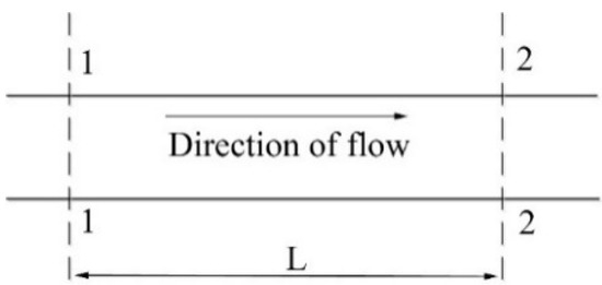
Figure 4. Locations of Cross-section 1-1 and Cross-section 2-2 along the pipe.

As shown in Figure 1, the instantaneous pressure head and discharge of the oscillating water flow at Cross-section 1-1 can be described as follows [33]:

$${\mathrm{H}}_1={\overline{\mathrm{H}}}_1+{\mathrm{h}}_1$$

(1)

$${\mathrm{Q}}_1={\overline{\mathrm{Q}}}_1+{\mathrm{q}}_1$$

(2)

where ${\mathrm{H}}_1$ is the instantaneous pressure head (m); ${\overline{\mathrm{H}}}_1$ is the average pressure head, which is the average of all the instantaneous pressure heads (m); ${\mathrm{h}}_1$ is the instantaneous pressure head deviation from the average (m); ${\mathrm{Q}}_1$ is the instantaneous discharge (m³/s); ${\overline{\mathrm{Q}}}_1$ is the average discharge, which is the average of all the instantaneous discharges (m³/s); and ${\mathrm{q}}_1$ is the instantaneous discharge deviation from the average (m³/s).

The relationship between the instantaneous discharge and velocity at Cross-section 1-1 is as follows:

$${\mathrm{Q}}_1=\mathrm{A}\times {\mathrm{V}}_1$$

(3)

where ${\mathrm{V}}_1$ is the instantaneous velocity (m/s); and A is the cross-sectional area of the flow in the pipe (m²).

According to Equations (2) and (3), the instantaneous velocity, ${\mathrm{V}}_1$, can be expressed as follows:

$${\mathrm{V}}_1={\overline{\mathrm{V}}}_1+{\mathrm{v}}_1$$

(4)

where ${\overline{\mathrm{V}}}_1$ is the average velocity, which is the average of all the instantaneous velocities (m/s); and ${\mathrm{v}}_1$ is the instantaneous velocity deviation from the average (m/s).

Equations (1)–(4) show that the oscillating water flow has constant features as well as variable features. The average instantaneous pressure head, discharge, and velocity are the constant features of the oscillating water flow. The instantaneous pressure head deviation from the average, the instantaneous discharge deviation from the average, and the instantaneous velocity deviation from the average are the variable features of the oscillating water flow.

The instantaneous pressure head deviation from the average, ${\mathrm{h}}_1$, the instantaneous discharge deviation from the average, ${\mathrm{q}}_1$, and the instantaneous velocity deviation from the average, ${\mathrm{v}}_1$, can be expressed as follows:

$${\mathrm{h}}_1={\mathrm{h}}_1^{*}\sin \left(\mathsf{\omega }\mathrm{t}\right)$$

(5)

$${\mathrm{q}}_1={\mathrm{q}}_1^{*}\sin \left(\mathsf{\omega }\mathrm{t}\right)$$

(6)

$${\mathrm{v}}_1={\mathrm{v}}_1^{*}\sin \left(\mathsf{\omega }\mathrm{t}\right)$$

(7)

where sin(ωt) is the sine function; ${\mathrm{h}}_1^{*}$ is the amplitude of the pressure head (m); ${\mathrm{q}}_1^{*}$ is the amplitude of the discharge (m³/s); ${\mathrm{v}}_1^{*}$ is the amplitude of the velocity (m/s); ω is the frequency of the oscillating water flow (rad/s), and t is time (s). Further, ω is related to P, as follows:

$$\mathsf{\omega }=\frac{2\mathsf{\pi }}{\mathrm{P}}$$

(8)

where P is the period of the oscillating water flow (s).

When $\sin \left(\mathsf{\omega }\mathrm{t}\right)=1$, the maximum instantaneous pressure head, discharge, and velocity can be obtained from Equations (1)–(7). Similarly, when $\sin \left(\mathsf{\omega }\mathrm{t}\right)=-1$, the minimum instantaneous pressure head, discharge, and velocity can be obtained by Equations (1)–(7).

When the oscillating water flows along the pipe, the average pressure head and the amplitude of the pressure head at Cross-section 2-2 can be described as follows:

$${\overline{\mathrm{H}}}_2={\overline{\mathrm{H}}}_1-{\overline{\mathrm{H}}}_{\mathrm{f}}$$

(9)

$${\mathrm{h}}_2^{*}={\mathrm{h}}_1^{*}-{\mathrm{h}}_{\mathrm{f}}^{*}$$

(10)

where ${\overline{\mathrm{H}}}_2$ is the average pressure head at Cross-section 2-2 (m); ${\overline{\mathrm{H}}}_1$ is the average pressure head at Cross-section 1-1 (m); ${\overline{ \mathrm{H}}}_{\mathrm{f}}$ is the average pressure head loss between Cross-section 1-1 and Cross-section 2-2 along the pipe; ${\mathrm{h}}_2^{*}$ is the amplitude of the pressure head at Cross-section 2-2 (m); ${\mathrm{h}}_1^{*}$ is the amplitude of the pressure head at Cross-section 1-1 (m); ${\mathrm{h}}_{\mathrm{f}}^{*}$ is the amplitude of the pressure head loss between Cross-section 1-1 and Cross-section 2-2 along the pipe.

According to Equations (1), (5), (9), and (10), the average pressure head loss and the amplitude of the pressure head loss are the keys to obtain the instantaneous pressure head of the oscillating water flow at Cross-section 2-2.

Under the condition of constant water flow, several formulas, such as the Darcy–Weisbach and the Hazen–Williams formulas, are widely used in irrigation engineering to calculate the pressure head loss [34,35,36,37]. These formulas can also be used to calculate the average pressure head loss of oscillating water flow with high accuracy. Therefore, the next step is to set up an empirical equation for the amplitude of the pressure head loss of oscillating water flow of different types of pipe.

2.3. Dimensional Analysis

Buckingham’s pi-theorem is an effective way to solve complex hydraulic problems. By analyzing the relationship between physical parameters, the theorem can be used to develop physical equations that describe the movement of water flow [38,39,40]. For a more comprehensive analysis of a hydraulics problem, according to Buckingham’s pi-theorem, the physical parameters should include the kinematic properties of water, physical properties of water, and the geometric properties of the boundary. All the physical parameters are to be listed in a relational expression and each physical parameter is expressed in terms of the dimensions mass (M), length (L), and time (T), as shown in Equation (11) and Table 2.

$${\mathrm{h}}_{\mathrm{f}}^{*}=\mathsf{\phi }\left({\overline{\mathrm{V}}}_1,{ \mathrm{v}}_1^{*},\mathrm{P},\mathrm{g},\mathsf{\upsilon },\mathsf{\rho },\mathrm{E},\mathrm{D},\mathsf{\delta },\mathrm{L}\right)$$

(11)

Table 2. Physical parameters that affect the amplitude of the pressure head loss of oscillating water flow.

Type of Physical Parameter	Symbol	Parameter	Dimension	Unit
Dependent variable	${\mathrm{h}}_{\mathrm{f}}{}^{*}$	Amplitude of the pressure head loss between Cross-section 1-1 and Cross-section 2-2 along the pipe	L	m
Independent variables	${\overline{\mathrm{V}}}_1$	Average velocity at Cross-section 1-1	${\mathrm{LT}}^{-1}$	$\mathrm{m}/\mathrm{s}$
	${\mathrm{v}}_1^{*}$	Amplitude of velocity at Cross-section 1-1	${\mathrm{LT}}^{-1}$	$\mathrm{m}/\mathrm{s}$
	$\mathrm{P}$	Period of oscillating water flow	T	s
	g	Acceleration due to gravity	${\mathrm{LT}}^{-2}$	$\mathrm{m}/{\mathrm{s}}^2$
	$\mathsf{\upsilon }$	Kinematic viscosity of water	${\mathrm{L}}^2{\mathrm{T}}^{-1}$	${\mathrm{m}}^2/\mathrm{s}$
	$\mathsf{\rho }$	Density of water	${\mathrm{ML}}^{-3}$	$\mathrm{kg}/{\mathrm{m}}^3$
	E	Modulus of elasticity of the pipe material	${\mathrm{ML}}^{-1}{\mathrm{T}}^{-2}$	$\mathrm{N}/{\mathrm{m}}^2$
	D	Internal pipe diameter	L	m
	$\mathsf{\delta }$	Thickness of the pipe wall	L	m
	L	Length of pipe between Cross-section 1-1 and Cross-section 2-2	L	m

Then, m physical parameters are selected from n physical parameters as the basic physical parameters. The remaining physical parameters and the basic physical parameters constitute n-m dimensionless $\mathsf{\pi }$ terms. The exponent of each dimensionless $\mathsf{\pi }$ term is calculated by the following equation:

$$\mathsf{\pi }=\frac{{\mathrm{x}}_{\mathrm{n}-\mathrm{m}}}{{\mathrm{x}}_1^{\mathrm{a}}{\mathrm{x}}_2^{\mathrm{b}}\cdots {\mathrm{x}}_{\mathrm{m}}^{\mathrm{r}}}$$

(12)

where ${\mathrm{x}}_1$, ${\mathrm{x}}_2$, and ${\mathrm{x}}_{\mathrm{m}}$ are the basic physical parameters; $\mathrm{a}$, $\mathrm{b}$, and $\mathrm{r}$ are the exponents of these basic physical parameters, respectively. In this study, the kinematic viscosity of water $\mathsf{\upsilon }$, density of water $\mathsf{\rho }$, and the internal pipe diameter D have been selected as the basic physical parameters. The remaining eight physical parameters and three basic physical parameters constitute eight dimensionless $\mathsf{\pi }$ terms, and the relevant indexes of each $\mathsf{\pi }$ term have been determined according to Equation (12), as shown in Table 3.

Table 3. Dimensionless $\mathsf{\pi }$ terms associated with the amplitude of the pressure head loss.

Pi Term	π1	π2	π3	π4	π5	π6	π7	π8
Expression	$\frac{{\mathrm{h}}_{\mathrm{f}}^{*}}{\mathrm{D}}$	$\frac{{\overline{\mathrm{V}}}_1\mathrm{D}}{\mathsf{\upsilon }}$	$\frac{{\mathrm{v}}_1^{*}\mathrm{D}}{\mathsf{\upsilon }}$	$\frac{\mathrm{P}\mathsf{\upsilon }}{{\mathrm{D}}^2}$	$\frac{{\mathrm{gD}}^3}{{\mathsf{\upsilon }}^2}$	$\frac{{\mathrm{ED}}^2}{{\mathsf{\rho }\mathsf{\upsilon }}^2}$	$\frac{\mathsf{\delta }}{\mathrm{D}}$	$\frac{\mathrm{L}}{\mathrm{D}}$

Substituting the dimensionless $\mathsf{\pi }$ terms in Table 3 into Equation (11) gives

$$\frac{{\mathrm{h}}_{\mathrm{f}}^{*}}{\mathrm{D}}=\mathsf{\phi }\left(\frac{{\overline{\mathrm{V}}}_1\mathrm{D}}{\mathsf{\upsilon }},\frac{{\mathrm{v}}_1^{*}\mathrm{D}}{\mathsf{\upsilon }},\frac{\mathrm{P}\mathsf{\upsilon }}{{\mathrm{D}}^2},\frac{{\mathrm{gD}}^3}{{\mathsf{\upsilon }}^2},\frac{{\mathrm{ED}}^2}{{\mathsf{\rho }\mathsf{\upsilon }}^2},\frac{\mathsf{\delta }}{\mathrm{D}},\frac{\mathrm{L}}{\mathrm{D}}\right)$$

(13)

2.4. Statistical Tests of Data

Statistical Product and Service Solutions (SPSS) is a software developed by IBM for statistical analysis, data mining, prediction analysis and decision support tasks. The next step is to conduct statistical tests on the data of the dimensionless $\mathsf{\pi }$ terms that have been obtained by the dimensional analysis of the physical parameters of oscillating water flow and pipe used in the experiments. Then, the data of the dimensionless $\mathsf{\pi }$ terms have been transformed using a logarithmic function, and a linear regression model has been fitted to the data using the SPSS software.

2.4.1. Multicollinearity Test

The value of the variance inflation factor (VIF) can indicate whether there is or there is no multicollinearity between each independent variable. From Table 4, it can be seen that the value of the VIF of each independent variable is less than 5. This is an indication that there is no multicollinearity between each independent variable [41].

Table 4. Values of variance inflation factor (VIF).

Pi term	${\mathsf{\pi }}_1$	${\mathsf{\pi }}_2$	${\mathsf{\pi }}_3$	${\mathsf{\pi }}_4$	${\mathsf{\pi }}_5$	${\mathsf{\pi }}_6$	${\mathsf{\pi }}_7$
VIF	2.713	2.504	3.287	3.098	4.182	1.689	1.690

2.4.2. Normality Test

The normal probability–probability plot of standardized residual (p-p plot) can indicate whether the residual among variables conforms to the normal distribution. From Figure 5, it can be seen that the points are basically distributed along a straight line. This is an indication that the residual of variables is normally distributed [42,43,44].

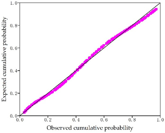
Figure 5. The normal probability–probability plot of standardized residual.

2.4.3. Heteroscedasticity Test

The distribution of the standardized predicted values and the standardized residual can indicate whether there is heteroscedasticity in the residual of the variables. From Figure 6, it can be seen that the points are randomly distributed and do not show an obvious trend, and the points almost fill the whole panel space. This is an indication that heteroscedasticity does not exist in the residual of the variables [45,46].

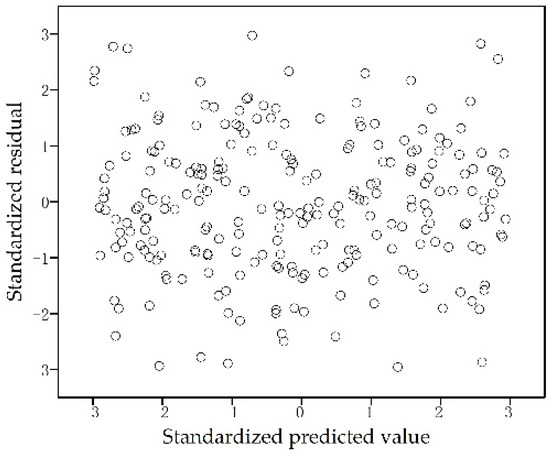
Figure 6. Distribution of standardized predicted values and standardized residual.

2.5. The Relative Error and Sensitivity Coefficient

The relative error is defined as:

$$\mathrm{Relative} \mathrm{error} = (\frac{\left|\mathrm{Measured} \mathrm{value}-\mathrm{Calculated} \mathrm{value}\right|}{\mathrm{Measured} \mathrm{value}}\times 100\%)$$

(14)

The sensitivity coefficient of each parameter can be calculated as follows [47,48]:

$$\mathrm{S}=\frac{{{\displaystyle \sum }}_{\mathrm{i}=1}^{\mathrm{n}-1}\frac{\left({\mathrm{Y}}_{\mathrm{i}+1}-{\mathrm{Y}}_{\mathrm{i}}\right)/{\mathrm{Y}}_0}{\left({\mathrm{K}}_{\mathrm{i}+1}-{\mathrm{K}}_{\mathrm{i}}\right)/100}}{n-1}$$

(15)

where S is the sensitivity coefficient; ${\mathrm{Y}}_0$ is the amplitude of the pressure head loss between Cross-section 1-1 and Cross-section 2-2 along the pipe as calculated by Equation (17) for the initial values of all parameters (m); ${\mathrm{Y}}_{\mathrm{i}}$ is the amplitude of the pressure head loss calculated by Equation (17) after the ith change of the target parameter when the other parameters remain unchanged at the initial value (m); ${\mathrm{Y}}_{\mathrm{i}+1}$ is the amplitude of the pressure head loss calculated by Equation (17) after the (i + 1)th change of the target parameter when the other parameters remain unchanged at the initial value (m); ${\mathrm{K}}_{\mathrm{i}}$ is the changed percent ratio of the target parameter after the ith change (%); ${\mathrm{K}}_{\mathrm{i}+1}$ is the changed percent ratio of the target parameter after the (i + 1)th change (%).

3. Results and Discussion

3.1. Results

The coefficients of Equation (13) have been determined by linear regression, thereby generating the following empirical equation for the amplitude of the pressure head loss:

$$\frac{{\mathrm{h}}_{\mathrm{f}}^{*}}{\mathrm{D}}=0.00938{\left(\frac{{\overline{\mathrm{V}}}_1\mathrm{D}}{\mathsf{\upsilon }}\right)}^{0.847}{\left(\frac{{\mathrm{v}}_1^{*}\mathrm{D}}{\mathsf{\upsilon }}\right)}^{1.034}{\left(\frac{\mathrm{P}\mathsf{\upsilon }}{{\mathrm{D}}^2}\right)}^{-0.035}{\left(\frac{{\mathrm{gD}}^3}{{\mathsf{\upsilon }}^2}\right)}^{-1.063}{\left(\frac{{\mathrm{ED}}^2}{{\mathsf{\rho }\mathsf{\upsilon }}^2}\right)}^{-0.012}{\left(\frac{\mathsf{\delta }}{\mathrm{D}}\right)}^{-0.022}{\left(\frac{\mathrm{L}}{\mathrm{D}}\right)}^{1.013}$$

(16)

The correlation coefficient, R², of Equation (16) is 0.992. This is an indication that the calculated amplitudes of the pressure head loss using Equation (16), and the experimental data are in very good agreement. Table 5 shows the results of the regression analysis for each dimensionless $\mathsf{\pi }$ term. Since $p<0.05$ for all the terms, this is an indication that all the terms have significant influences on the results of the regression analyses.

Table 5. Results of regression analyses for all the terms in Equation (14).

Term in Equation (14)	Coefficient	Standard Deviation	T test	p-Value
Constant	0.00938	0.076	−26.688	$<0.05$
${\overline{\mathrm{V}}}_1\mathrm{D}/\mathsf{\upsilon }$	0.847	0.027	31.576	$<0.05$
${\mathrm{v}}_1^{*}\mathrm{D}/\mathsf{\upsilon }$	1.034	0.017	60.56	$<0.05$
$\mathrm{P}\mathsf{\upsilon }/{\mathrm{D}}^2$	−0.035	0.025	−1.404	$<0.05$
${\mathrm{gD}}^3/{\mathsf{\upsilon }}^2$	−1.063	0.024	−43.525	$<0.05$
${\mathrm{ED}}^2/{\mathsf{\rho }\mathsf{\upsilon }}^2$	−0.012	0.014	−0.822	$<0.05$
$\mathsf{\delta }/\mathrm{D}$	−0.022	0.015	−1.464	$<0.05$
$\mathrm{L}/\mathrm{D}$	1.013	0.013	77.786	$<0.05$

Substituting $\mathrm{g}=9.8 \mathrm{m}/{\mathrm{s}}^2$, $\mathsf{\upsilon }=1.01\times {10}^{-6} {\mathrm{m}}^2/\mathrm{s}$, and $\mathsf{\rho }=1000 \mathrm{kg}/{\mathrm{m}}^3$ into Equation (16) gives

$${\mathrm{h}}_{\mathrm{f}}^{*}=0.0009{\left({\overline{\mathrm{V}}}_1\right)}^{0.847}{\left({\mathrm{v}}_1^{*}\right)}^{1.034}{\left(\mathrm{P}\right)}^{-0.035}{\left(\mathrm{E}\right)}^{-0.012}{\left(\mathrm{D}\right)}^{-1.253}{\left(\mathsf{\delta }\right)}^{-0.022}{\left(\mathrm{L}\right)}^{1.013}$$

(17)

3.1.1. Validation of the Empirical Equation

In order to verify the accuracy of the calculated amplitudes of the pressure head loss by the empirical Equation (17), validation experiments have been designed, and the parameters of each experimental case of the validation experiments are different from the original experiments (Section 2.1.2). The experiment equipment and the arrangement of the pressure transducers for the validation experiments are the same as those in the original experiments (Section 2.1.1). The pipe used in the experimental Case T1 is PE (polyethylene) drip tape. The pipe used in the experimental Case T2 is ABS (acrylonitrile-butadiene-styrene) pipe. The pipe used in the experimental Case T3 is PVC (polyvinyl chloride) pipe. The pipe used in the experimental Case T4 is PS (polystyrene) pipe. Finally, the pipe used in the experimental Case T5 is PP (perspex) pipe. Table 6 shows the physical parameters of the oscillating water flow and the pipe used the validation experiments.

Table 6. Physical parameters of oscillating water flow and pipe used in the validation experiments.

Case	${\overline{\mathbf{H}}}_1\left(\mathbf{m}\right)$	${\mathbf{h}}_1^{*}\left(\mathbf{m}\right)$	${\overline{\mathbf{V}}}_1$$(\mathbf{m}/\mathbf{s})$	${\mathbf{v}}_1^{*}$$(\mathbf{m}/\mathbf{s})$	P(s)	$\mathbf{E}({10}^9\mathbf{N}/{\mathbf{m}}^2)$	D(m)	$\mathsf{\delta }$	L(m)
T1	5.12	2.27	0.61	0.26	43	0.8	0.0246	0.0002	48
T2	13.9	9.11	1.87	0.80	59	1.7	0.0544	0.0043	48
T3	11.88	10.83	1.98	1.09	30	2.6	0.0678	0.0036	48
T4	23.20	11.51	2.15	0.98	92	5	0.046	0.002	48
T5	46.49	8.27	2.44	0.35	76	6	0.029	0.0015	48

Figure 7 shows the comparisons of the measured and calculated amplitudes of the pressure head loss along the pipe for Cases T1, T2, T3, T4, and T5. It can be seen that the amplitude of the pressure head loss increases with increasing length of pipe. The amplitude of the pressure head loss of the oscillating water flow is caused by two types of energy loss. On the one hand, when the oscillating water flows along the pipe, there is energy loss caused by the work done by the water flow to overcome the frictional resistance of the pipe. On the other hand, the instantaneous pressure head of the oscillating water flow is changing constantly, which leads to the energy loss caused by the intense mixing and collision of particles in water. From Figure 7, it can be seen that the function type of the optimal fits to the measured amplitudes of Cases T1, T2, T3, T4, and T5 are not the same. The function type of the optimal fit to the measured amplitudes of Case T1 is power. The function type of the optimal fits to the measured amplitudes of Cases T2 and T5 is polynomial. The function type of the optimal fit to the measured amplitudes of Case T3 is logarithmic. The function type of the optimal fit to the measured amplitudes of Case T4 is exponential. However, the function type of the optimal fit to the calculated amplitudes by Equation (17) for Cases T1, T2, T3, T4, and T5 is linear. It can be seen that the calculated amplitudes by the empirical equation developed in this study (17) approximates the measured amplitudes in the form of a linear function.

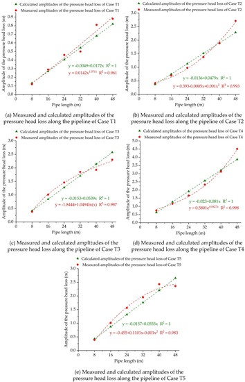
Figure 7. Comparisons of measured and calculated amplitudes of the pressure head loss along the pipe for (a) Case T1, (b) Case T2, (c) Case T3, (d) Case T4, and (e) Case T5.

Using the empirical equation for the amplitude of the pressure head loss (Equation (17)), Table 7 shows the relative errors between the measured and the calculated amplitudes of the pressure head loss for Cases T1, T2, T3, T4, and T5.

Table 7. The measured and calculated amplitudes of the pressure head loss along the pipe for Cases T1, T2, T3, T4, and T5.

Case	Item	Location Along Pipe (m)
		8	16	24	32	40	48
T1	Calculated amplitude (m)	0.13	0.27	0.41	0.54	0.68	0.82
	Measured amplitude (m)	0.12	0.29	0.46	0.5	0.81	0.88
	Relative error (%)	8.33	6.90	10.87	8.00	16.05	6.82
T2	Calculated amplitude (m)	0.37	0.75	1.13	1.52	1.9	2.29
	Measured amplitude (m)	0.41	0.7	0.98	1.38	1.89	2.71
	Relative error (%)	9.76	7.14	15.31	10.14	0.53	15.50
T3	Calculated amplitude (m)	0.42	0.85	1.28	1.71	2.14	2.57
	Measured amplitude (m)	0.38	1.01	1.46	1.85	1.93	2.3
	Relative error (%)	10.53	15.84	12.33	7.57	10.88	11.74
T4	Calculated amplitude (m)	0.63	1.27	1.92	2.57	3.22	3.87
	Measured amplitude (m)	0.74	1.16	1.66	2.33	3.12	4.51
	Relative error (%)	14.86	9.48	15.66	10.30	3.21	14.19
T5	Calculated amplitude (m)	0.43	0.87	1.31	1.76	2.21	2.65
	Measured amplitude (m)	0.39	1.01	1.56	1.95	2.43	2.36
	Relative error (%)	10.26	13.86	16.03	9.74	9.05	12.29

As shown in Table 7, the average relative error (Equation (14)) between the measured and the calculated amplitudes of the pressure head loss by the empirical equation is 10.77%. These results show that the relative error of the calculated amplitude of the pressure head loss by the empirical equation is small, and the calculated and measured amplitudes of the pressure head loss are close to each other. This is an indication that the amplitude of the pressure head loss calculated by the empirical equation is accurate.

3.1.2. Sensitivity Analysis of Empirical Equation

According to Equation (17), the amplitude of the pressure head loss between Cross-section 1-1 and Cross-section 2-2 along the pipe, ${\mathrm{h}}_{\mathrm{f}}{}^{*}$, can be calculated using the seven parameters. Therefore, the sensitivity analyses of Equation (17) have been carried out by changing these seven parameters. The average measured value of each parameter in all the experiments (i.e., the experiments described in Section 2.1.2 and Section 3.1.1) is defined as the initial value of the parameter. The initial value of each parameter is then changed by a fixed increment of $\pm$10% up to $\pm$50%. Table 8 shows the initial value of each parameter and the value range after the initial value of each parameter is changed.

Table 8. Initial value of each parameter and the value range of each parameter.

Parameter	Initial Value	Value Range of Each Parameter
Average velocity at Cross-section 1-1 (${\overline{\mathrm{V}}}_1$)	3.24	1.62–4.86
Amplitude of velocity at Cross-section 1-1 (${\mathrm{v}}_1^{*}$)	0.62	0.31–0.93
Period of oscillating water flow (P)	60.32	30.16–90.48
Modulus of elasticity of the pipe material (E)	3.18	1.59–4.77
Internal pipe diameter (D)	0.056	0.0280–0.0840
Thickness of the pipe wall ($\mathsf{\delta }$)	0.0026	0.0013–0.0038
Length of pipe between Cross-section 1-1 and Cross-section 2-2 (L)	28.46	14.23–42.69

Table 9 gives the sensitivity classification according to the value of the sensitivity coefficient, as follows [49,50]:

Table 9. Sensitivity classification.

$\mathbf{Value} \mathbf{of} \left|\mathbf{S}\right|$	$\left|\mathbf{S}\right| \ge 1$	$0.2 \le \left|\mathbf{S}\right| < 1$	$0.05 \le \left|\mathbf{S}\right| < 0.2$	$0 \le \left|\mathbf{S}\right| < 0.05$
Sensitivity classification	highly sensitive	sensitive	medium sensitive	insensitive

Table 10 shows the sensitivity classification of the seven parameters in Equation (17). It can be seen that the amplitude of velocity, the internal pipe diameter, and the length of pipe are classified as highly sensitive. The average velocity, the period of oscillating water flow, and the modulus of elasticity of the pipe material are classified as sensitive. The thickness of the pipe wall is classified as medium sensitive.

Table 10. Sensitivity classification of the seven parameters in Equation (17).

Parameter	Sensitivity Coefficient	Sensitivity Classification
Average velocity at Cross-section 1-1 (${\overline{\mathrm{V}}}_1$)	0.85	sensitive
Amplitude of velocity at Cross-section 1-1 (${\mathrm{v}}_1^{*}$)	1.03	highly sensitive
Period of oscillating water flow (P)	−0.37	sensitive
Modulus of elasticity of the pipe material (E)	−0.22	sensitive
Internal pipe diameter (D)	−1.55	highly sensitive
Thickness of the pipe wall ($\mathsf{\delta }$)	−0.13	medium sensitive
Length of pipe between Cross-section 1-1 and Cross-section 2-2 (L)	1.01	highly sensitive

3.2. Discussion

In this study, an empirical equation for the amplitude of the pressure head loss of oscillating water flow in different types of pipes has been developed. In order to verify the accuracy of the calculated results from the empirical equation, five cases (i.e., Cases T1, T2, T3, T4, and T5) have been tested. The results show that the empirical equation can be used to calculate the amplitude of the pressure head loss of oscillating water flow in different types of pipes accurately. For the empirical equation developed in this study, the sensitivity of the model parameters has been analyzed. Further, for all the experiments carried out in this study, as the water flowed in the pipe, there was no loss of water. However, due to the need of the actual irrigation on-site, multiple outlet pipes have sometimes been used, and as the water flowed in the pipe, there was loss of water. Under the condition of constant water flow, the Christiansen’s factor is widely used in the calculation of pressure head loss of multiple outlet pipes. After a long time of development, some studies have adjusted the calculation equation of the Christiansen’s factor and developed some improved methods [51,52,53]. These methods can also be used to calculate the average pressure head loss of oscillating water flow with high accuracy. But these methods cannot calculate the amplitude of the pressure head loss of oscillating water flow of multiple outlet pipes accurately. Therefore, further research should be carried out to adjust the calculation equation of Christiansen’s factor, so that it can calculate the amplitude of the pressure head loss of oscillating water flow of multiple outlet pipes accurately. It is of great significance for both the application and operation of oscillating water flow in irrigation engineering.

4. Conclusions

In this study, an empirical equation for the amplitude of the pressure head loss of the oscillating water flow in different types of pipe has been developed. Further, the accuracy of the empirical equation has been verified by the validation experiments and the sensitivity of each parameter in the empirical equation has been analyzed. The main conclusions are as follows:

The average relative error between the measured and the calculated amplitudes of the pressure head loss by the empirical equation is 10.77%. Since the relative errors are small, it is an indication that the amplitudes of the pressure head loss calculated by the empirical equation are accurate.

The amplitude of velocity, the internal pipe diameter, and the length of pipe are classified as highly sensitive. The average velocity, the period of oscillating water flow, and the modulus of elasticity of the pipe material are classified as sensitive. The thickness of the pipe wall is classified as medium sensitive.

The empirical equation developed in this study can be used to calculate the amplitude of the pressure head loss of oscillating water flow in different types of pipes. It improves the computing efficiency significantly and provides a theoretical basis for the application of oscillating water flow in irrigation engineering and the optimal design of irrigation pipe networks.

References

- Woltering, L.; Ibrahim, A.; Pasternak, D.; Ndjeunga, J. The economics of low pressure drip irrigation and hand watering for vegetable production in the Sahel. Agric. Water Manag. 2011, 99, 67–73. [Google Scholar] [CrossRef]
- Marsh, B.; Dowgert, M.; Hutmacher, R.; Phene, C.J. Low-pressure drip system in reduced tillage cotton. WIT Ecol. Environ. 2007, 103, 73–80. [Google Scholar]
- Kranz, W.L.; Eisenhauer, D.E.; Retka, M.T. Water and energy-conservation using irrigation scheduling with center-pivot irrigation systems. Agric. Water Manag. 1992, 22, 325–334. [Google Scholar] [CrossRef]
- O’Shaughnessy, S.A.; Evett, S.R.; Andrade, M.A.; Workneh, F.; Price, J.A.; Rush, C.M. Site-specific variable-rate irrigation as a means to enhance water use efficiency. Trans. ASABE 2016, 59, 239–249. [Google Scholar]
- Singh, A.K.; Sharma, S.P.; Upadhyaya, A.; Rahman, A.; Sikka, A.K. Performance of low energy water application device. Water Resour. Manag. 2010, 24, 1353–1362. [Google Scholar] [CrossRef]
- Masseroni, D.; Arbat, G.; de Lima, I.P. Editorial—Managing and Planning Water Resources for Irrigation: Smart-Irrigation Systems for Providing Sustainable Agriculture and Maintaining Ecosystem Services. Water 2020, 12, 263. [Google Scholar] [CrossRef]
- Wei, Q.S.; Lu, G.; Liu, J.; Shi, Y.S.; Dong, W.C.; Huang, S.H. Evaluations of emitter clogging in drip irrigation by two-phase flow simulations and laboratory experiments. Comput. Electron. Agric. 2008, 63, 294–303. [Google Scholar]
- Oron, G.; Demalach, J.; Hoffman, Z.; Cibotaru, R. Subsurface microirrigation with effluent. J. Irrig. Drain. Eng. ASCE 1991, 117, 25–36. [Google Scholar] [CrossRef]
- Zhai, G.L.; Lv, M.C.; Wang, H.; Xiang, H.A. Plugging of microirrigation system and its prevention. Trans. Chin. Soc. Agric. Eng. 1999, 15, 144–147. [Google Scholar]
- Shamshery, P.; Winter, A.G. Shape and form optimization of on-line pressure-compensating drip emitters to achieve lower activation pressure. J. Mech. Des. 2018, 140, 035001. [Google Scholar] [CrossRef]
- Sayyadi, H.; Nazemi, A.H.; Sadraddini, A.A.; Delirhasannia, R. Characterising droplets and precipitation profiles of a fixed spray-plate sprinkler. Biosyst. Eng. 2014, 119, 13–24. [Google Scholar] [CrossRef]
- Seginer, I.; Kantz, D.; Nir, D. The distortion by wind of the distribution patterns of single sprinklers. Agric. Water Manag. 1991, 19, 341–359. [Google Scholar] [CrossRef]
- Li, G.Y.; Wang, J.D.; Alam, M.; Zhao, G.Y. Influence of geometrical parameters of labyrinth flow path of drip emitters on hydraulic and anti-clogging performance. Trans. ASABE 2006, 49, 637–643. [Google Scholar] [CrossRef]
- Yu, L.M.; Li, N.; Liu, X.G.; Yang, Q.L.; Li, Z.Y.; Long, J. Influence of dentation angle of labyrinth channel of drip emitters on hydraulic and anti-clogging performance. Irrig. Drain. 2019, 68, 256–267. [Google Scholar] [CrossRef]
- Zhang, J.; Zhao, W.H.; Tang, Y.P.; Lu, B.H. Anti-clogging performance evaluation and parameterized design of emitters with labyrinth channels. Comput. Electron. Agric. 2010, 74, 59–65. [Google Scholar] [CrossRef]
- Zhang, J.; Zhao, W.H.; Tang, Y.P.; Lu, B.H. Structural optimization of labyrinth-channel emitters based on hydraulic and anti-clogging performances. Irrig. Sci. 2011, 29, 351–357. [Google Scholar] [CrossRef]
- Liu, J.; Yuan, S.; Li, H.; Zhu, X. Combination uniformity improvement of impact sprinkler. Trans. Chin. Soc. Agric. Eng. 2011, 27, 107–111. [Google Scholar]
- Li, H.; Jiang, Y.; Xu, M.; Li, Y.; Chen, C. Effect on hydraulic performance of low-pressure sprinkler by an intermittent water dispersion device. Trans. ASABE 2016, 59, 521–532. [Google Scholar]
- Yuan, S.; Wei, Y.; Li, H.; Xiang, Q. Structure design and experiments on the water distribution of the variable-rate sprinkler with non-circle nozzle. Trans. Chin. Soc. Agric. Eng. 2010, 26, 149–153. [Google Scholar]
- Zhang, L.; Wu, P.; Zhu, D.; Zheng, C. Effect of oscillating pressure on labyrinth emitter clogging. Irrig. Sci. 2017, 35, 267–274. [Google Scholar] [CrossRef]
- Zheng, C.; Wu, P.T.; Zhang, L.; Zhu, D.L.; Zhao, X.; An, B.D. Particles movement characteristics in labyrinth channel under different dynamic water pressure modes. Trans. Chin. Soc. Agric. Mach. 2017, 48, 294–301. [Google Scholar]
- Yu, L.M.; Li, N.; Liu, X.G.; Yang, Q.L.; Long, J. Influence of flushing pressure, flushing frequency and flushing time on the service life of a labyrinth-channel emitter. Biosyst. Eng. 2018, 172, 154–164. [Google Scholar] [CrossRef]
- Zhang, K.; Song, B.; Zhu, D. The influence of sinusoidal oscillating water flow on sprinkler and impact kinetic energy Intensities of laterally-moving sprinkler irrigation systems. Water 2019, 11, 1325. [Google Scholar] [CrossRef]
- Hills, D.J.; Silveira, R.C.M.; Wallender, W.W. Oscillating pressure for improving application uniformity of spray emitters. Trans. ASABE 1986, 29, 1080–1085. [Google Scholar] [CrossRef]
- Hills, D.J.; Gu, Y.P.; Wallender, W.W. Sprinkler uniformity for oscillating low water-pressure. Trans. ASABE 1987, 30, 729–734. [Google Scholar] [CrossRef]
- Buchin, A.F.; Pons, S.J.; Hills, D.J.; Abudu, S. Improving Water Application Efficiency in the Landscape through Pressure Oscillation. April 2004. Available online: https://www.researchgate.net/publication/237342500 (accessed on 1 April 2019).
- Tijsseling, A.S. Water hammer with fluid–structure interaction in thick-walled pipes. Comput. Struct. 2007, 85, 844–851. [Google Scholar] [CrossRef]
- Ghidaoui, M.S.; Mansour, S.G.S.; Zhao, M. Applicability of quasisteady and axisymmetric turbulence models in water hammer. J. Hydraul. Eng. 2002, 128, 917–924. [Google Scholar] [CrossRef]
- Zhang, B.; Wan, W.; Shi, M. Experimental and numerical simulation of water hammer in gravitational pipe flow with continuous air entrainment. Water 2018, 10, 928. [Google Scholar] [CrossRef]
- Kochupillai, J.; Ganesan, N.; Padmanabhan, C. A new finite element formulation based on the velocity of flow for water hammer problems. Int. J. Press. Vessel. Pip. 2005, 82, 1–14. [Google Scholar] [CrossRef]
- Besharat, M.; Teresa, V.M.; Ramos, H. Experimental study of air vessel behavior for energy storage or system protection in water hammer events. Water 2017, 9, 63. [Google Scholar] [CrossRef]
- Guo, Q.; Zhou, J.; Li, Y.; Guan, X.; Liu, D.; Zhang, J. Fluid-Structure Interaction Response of a Water Conveyance System with a Surge Chamber during Water Hammer. Water 2020, 12, 1025. [Google Scholar] [CrossRef]
- Zhang, K.; Song, B.; Zhu, D. The Development of a Calculation Model for the Instantaneous Pressure Head of Oscillating Water Flow in a Pipeline. Water 2019, 11, 1583. [Google Scholar] [CrossRef]
- Allen, R.G. Relating the Hazen-Williams and Darcy-Weisbach friction loss equations for pressurized irrigation. Appl. Eng. Agric. 1996, 12, 685–694. [Google Scholar] [CrossRef]
- Haktanır, T.; Ardıc¸lıog˘lu, M. Numerical modeling of Darcy–Weisbach friction factor and branching pipes problem. Adv. Eng. Softw. 2004, 35, 773–779. [Google Scholar] [CrossRef]
- Geem, Z.W.; Kim, J.H.; Loganathan, G.V. Harmony search optimization: Application to pipe network design. Int. J. Simul. Model. 2002, 22, 125–133. [Google Scholar] [CrossRef]
- Valiantzas, J.D. Modified Hazen–Williams and Darcy–Weisbach equations for friction and local head losses along irrigation laterals. J. Irrig. Drain. Eng. ASCE 2005, 131, 342–350. [Google Scholar] [CrossRef]
- Yurdem, H.; Demir, V.; Degirmencioglu, A. Development of a mathematical model to predict clean water head losses in hydrocyclone filters in drip irrigation systems using dimensional analysis. Biosyst. Eng. 2010, 105, 495–506. [Google Scholar] [CrossRef]
- Zitterell, D.B.; Frizzone, J.A.; Neto, O.R. Dimensional analysis approach to estimate local head losses in microirrigation connectors. Irrig. Sci. 2014, 32, 169–179. [Google Scholar] [CrossRef]
- Wang, Y.; Zhu, D.; Zhang, L.; Zhu, S. Simulation of Local Head Loss in Trickle Lateral Lines Equipped with In-line Emitters Based on Dimensional Analysis: Local head loss in trickle laterals lines. Irrig. Drain. 2018, 67, 572–581. [Google Scholar] [CrossRef]
- Sreen, N.; Purbey, S.; Sadarangani, P. Impact of culture, behavior and gender on green purchase intention. J. Retail. Consum. Serv. 2018, 41, 177–189. [Google Scholar] [CrossRef]
- Olive, D.J. Linear Regression; Springer International Publishing AG: Cham, Switzerland, 2017. [Google Scholar]
- Henderson, A.R. Testing experimental data for univariate normality. Clin. Chim. Acta 2006, 366, 112–129. [Google Scholar] [CrossRef] [PubMed]
- Bakar, S.A.; Nadarajah, S.; Adzhar, Z.A. Loss modeling using Burr mixtures. Empir. Econ. 2018, 54, 1503–1516. [Google Scholar]
- Sun, R.; Yuan, H.; Liu, X. Effect of heteroscedasticity treatment in residual error models on model calibration and prediction uncertainty estimation. J. Hydrol. 2017, 554, 680–692. [Google Scholar] [CrossRef]
- Cleasby, I.R.; Nakagawa, S. Neglected biological patterns in the residuals. Behav. Ecol. Sociobiol. 2011, 65, 2361–2372. [Google Scholar] [CrossRef]
- Sang, X.; Zhou, Z.; Wang, H.; Qin, D.; Zhai, Z.; Chen, Q. Development of Soil and Water Assessment Tool Model on Human Water Use and Application in the Area of High Human Activities, Tianjin, China. J. Irrig. Drain. Eng. ASCE 2010, 136, 23–30. [Google Scholar] [CrossRef]
- Wang, X.; Kang, F.; Li, J.; Wang, X. Inverse Parametric Analysis of Seismic Permanent Deformation for Earth-Rockfill Dams Using Artificial Neural Networks. Math. Probl. Eng. 2012, 2012, 1–19. [Google Scholar] [CrossRef]
- Lenhart, T.; Eckhardt, K.; Fohrer, N.; Frede, H.G. Comparison of two different approaches of sensitivity analysis. Phys. Chem. Earth 2002, 27, 645–654. [Google Scholar] [CrossRef]
- Yin, Y.; Wu, S.; Chen, G.; Dai, E. Attribution analyses of potential evapotranspiration changes in China since the 1960s. Theor. Appl. Climatol. 2010, 101, 19–28. [Google Scholar] [CrossRef]
- Scaloppi, E.J. Adjusted F factor for multiple-outlet pipes. J. Irrig. Drain. Eng. 1988, 114, 169–174. [Google Scholar] [CrossRef]
- Anwar, A.A. Factor G for pipelines with equally spaced multiple outlets and outflow. J. Irrig. Drain. Eng. 1999, 125, 34–38. [Google Scholar] [CrossRef]
- Ju, X.; Weckler, P.R.; Wu, P.; Zhu, D.; Wang, X.; Li, Z. New Simplified Approach for Hydraulic Design of Micro-Irrigation Paired Laterals. Trans. ASABE 2015, 58, 1521–1534. [Google Scholar]
© 2020 by the authors. Licensee MDPI, Basel, Switzerland. This article is an open access article distributed under the terms and conditions of the Creative Commons Attribution (CC BY) license (http://creativecommons.org/licenses/by/4.0/).