Abstract
Hydrological models, with different levels of complexity, have become inherent tools in water resource management. Conceptual models with low input data requirements are preferred for streamflow modeling, particularly in poorly gauged watersheds. However, the inadequacy of model structures in the hydrologic regime of a given watershed can lead to uncertain parameter estimation. Therefore, an understanding of the model parameters’ behavior with respect to the dominant hydrologic responses is of high necessity. In this study, we aim to investigate the parameterization of the HBV (Hydrologiska Byråns Vattenbalansavedelning) conceptual model and its influence on the model response in a semi-arid context. To this end, the capability of the model to simulate the daily streamflow was evaluated. Then, sensitivity and interdependency analyses were carried out to identify the most influential model parameters and emphasize how these parameters interact to fit the observed streamflow under contrasted hydroclimatic conditions. The results show that the HBV model can fairly reproduce the observed daily streamflow in the watershed of interest. However, the reliability of the model simulations varies from one year to another. The sensitivity analysis showed that each of the model parameters has a certain degree of influence on model behavior. The temperature correction factor (ETF) showed the lowest effect on the model response, while the sensitivity to the degree-day factor (DDF) highly depends on the availability of snow cover. Overall, the changes in hydroclimatic conditions were found to be mostly responsible for the annual variability of the optimal parameter values. Additionally, these changes seem to actuate the interdependency between the parameters of the soil moisture and the response routines, particularly Field Capacity (FC), the recession coefficient K0, the percolation coefficient (KPERC), and the upper reservoir threshold (UZL). The latter combines either to shrink the storage capacity of the model’s reservoirs under extremely high peak flows or to enlarge them under overestimated water supply, mainly provoked by abundant snow cover.
Keywords:
HBV model; conceptual; semi-arid; mountain; sensitivity analysis; interdependency analysis 1. Introduction
Mathematical models have been widely used in water resource-related applications, and they have become essential tools for management and planning purposes [1]. Various structures are available with different degrees of complexity from simple conceptual lumped models to more physically-based distributed ones [2,3,4,5,6,7,8]. Conceptual models based on physical concepts have been more attractive to the hydrological community due to their low requirements of input data and flexibility in application. However, serious questions were raised about the complexity related to model structures and parameters, and their eventual impact on the consistency of these models. Thus, many discussions have been conducted on whether simple structures or more complex models provide optimal estimations of streamflow [9,10,11,12]. Some studies have reported that models with complex structures do not always implicate superior performance compared to simple ones [1,13,14]. According to Abdulla and Al-Badranih [15] and Orth et al. [9], models that reasonably describe the water balance components with the simplest structure and adequate model parameters are preferable, particularly with fewer data requirements. The performance of lumped conceptual models, which are approximations of the real system with inherent uncertainties [10], can be comparable to even more physically based models in contexts of low-quality input data [9,16]. A trade-off between the complexity, efficiency, and data availability is unavoidable [1], particularly over watersheds in semi-arid regions with limited gauging networks.
Among the wide range of conceptual hydrologic models available in the literature, the HBV (Hydrologiska Byråns Vattenbalansavedelning) model has been tested and applied in a wide range of hydrological studies in numerous regions of different physiographic and climatic contexts [11]. The model was initially developed for flood warnings and runoff forecasting in Sweden [1,8]. Later on, the model structure gained trust around the world and multiple versions have become available [17,18,19,20,21]. The model was used to reproduce the water balance components and analyze their temporal variability [22,23]. In addition, numerous works have used the HBV model to assess climate change impact on water resources in different contexts [24,25,26,27], evaluate the impact of landscape characteristics and land cover changes on the runoff response [28,29], and to investigate the influence of geomorphologic characteristics on the groundwater modeling process [30]. In particular, the model showed significant potential for predicting streamflow in ungauged basins [11,31,32,33,34]. Overall, the HBV conceptual model was found to reliably perform under different climatic and physiographic contexts [17,35,36,37]. The worldwide applicability of the HBV model was made possible thanks to its low data requirements and its detailed physically sound structure [1,11]. The latter describes most of the significant physical processes that come into play for runoff generation [38]. Although they are of huge attractiveness in hydrologic modeling, these kinds of models can be quite challenging when used to simulate streamflow under certain circumstances. The comprehensive description of the hydrologic process within conceptual models increases the risk of overparameterization, which may constitute a significant constraint in terms of computing power and parameter uncertainty [10]. In particular, the relatively large number of free model parameters combined with structure inadequacies provokes parameter interdependency [10,39]. The former is one of the main factors responsible for the nonuniqueness issue, where multiple and unrealistic parameter combinations can yield equally good results [10,39,40,41,42,43].
The sensitivity analysis is a powerful tool that helps the modelers to understand the functioning of a certain hydrologic model in their respective hydroclimatic and physiographic contexts. Particularly, it allows the identification of the individual significance of each of the parameters to the final model output and, thus, the optimization of the parameterization of the model structure with respect to the dominant hydroclimatic process characterizing a given watershed [44,45]. Fewer studies were dedicated to comprehensive analyses of the HBV model sensitivity to each of its internal parameters [40,46,47,48], most of them were conducted in humid and sub-humid climatic contexts. To our knowledge, no previous study has covered this topic in a semi-arid region. Thus, the main aim of this paper was to investigate the sensitivity and parameter interdependency of the HBV conceptual model in a semi-arid mountainous watershed. To this end, the capability of the model to reproduce the daily observed streamflow was, firstly, tested through a calibration–validation exercise. The parameter set that was found to perform the best in most of the studied years, after validation, was used to examine the model sensitivity. Lastly, a bivariate analysis was carried out to highlight the interdependency and emphasize how the most influential parameters compensate each other to provide the most fitted model under contrasted hydroclimatic conditions.
2. Materials and Methods
2.1. Study Area
The Ait Ouchen watershed that lies within the limits of the Oum Er-Rbia river basin (OERB) in the center of Morocco was used in this study (Figure 1). The drained area is about 2427 km2, and it is located in the Atlas mountain range with elevations between 953 m and 3230 m.a.s.l. The main river of the watershed (El Abid) feeds Bin El Ouidane, one of the largest dams in Morocco, that contributes to hydropower generation [49,50] and supplies water to support the agriculture activities in irrigated areas [51,52]. The study area is predominantly semi-arid with a mean regional average of around 480 mm·year−1 [53]. The rainfall, characterized by a strong spatiotemporal variability over the mountainous region, is mostly generated under the combined effect of western advections and the orographic uplifting from the Atlas mountain [53]. Two distinct periods mark the annual cycle of rainfall: a wet period (November–April) and a dry period (June–September) separated by two transitory months (October and May). The smallest amounts of rainfall occur during the summer (June, July, and August) while the maximum totals usually take place during the winter months (December, January, and February). Nevertheless, stormy events are predominantly observed during summer and autumn generating high rainfall amounts that can exceed those recorded during the winter. Over high elevations of the Atlas Mountain, part of the precipitations occurs as snow. The latter exhibits a strong seasonality. It starts to take place in mid-November when the temperatures are low enough to allow snow occurrence and start to reduce in size in mid-April to completely vanish during summer [54]. Temperatures down to −9 °C are recorded during winter against a maximum of 41 °C during summer [50].
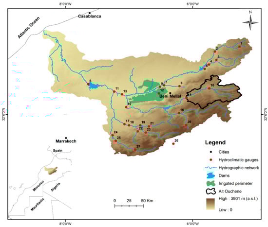
Figure 1.
The geographical setting of the study area. The brown area refers to the digital elevation model of the Oum Er-Rbia river basin (OERB).
2.2. Observed Data
The datasets used in this study were obtained from different sources. Daily rainfall and daily streamflow were delivered by the Oum Er-Rbia hydraulic Basin Agency (ABHOER). Most of the gauges managed by the ABHOER are intended for both rainfall and streamflow measurements. All available gauges are situated on the banks of the hydrographic network (Figure 1). The regional rainfall of the Ait Ouchene watershed was derived using data from the gauges located within the limits of the same watershed. The OERB suffers from the absence of consistent daily temperature data. Therefore, the average temperature of the Ait Ouchene watershed was estimated based on the lapse rate method, using a rate of 0.56 °C per 100 m of elevation estimated by Boudhar et al. [55] for mountainous watersheds close to Ait Ouchene. The long term mean monthly evapotranspiration values were estimated using the Thornthwaite formula, which considers potential evapotranspiration as a function of air temperature [56]. The lengths of all hydroclimatic data series were adjusted to match the span of available temperature data, which cover a period of nine hydrologic years (1 September–31 August) from 2001/2002 to 2009/2010. The interannual variability of hydroclimatic variables over the studied watershed is presented in Table 1.

Table 1.
Interannual variability of median Snow Cover Area (SCA), total rainfall, average temperature, and average streamflow anomalies over the study area.
2.3. MODIS Snow Cover Area (SCA)
Over the mountainous region of the OERB, there are no gauging stations for snow depth measurements. Satellite data are the only source available to derive information about snow cover. The MOD10A1 version 6 product, from Terra MODIS (Moderate-Resolution Imaging Spectroradiometer) satellite data [57], was used in this study to cope with the lack of snow in situ data. Since the early 2000s, the product provides daily maps of Snow Cover Area (SCA) at 500 m spatial resolution. However, daily maps are often affected by cloud coverage. Therefore, the original images were processed to fill missing and cloud covered grid-cells adopting the methodology reported in Marchane et al. [58] specifically developed for the Moroccan Atlas mountain range.
The performance of the MOD10A1 product against in situ data was assessed by Marchane et al. [58] over the Atlas mountain of Morocco, including the watershed case study. They have concluded that the SCA MODIS product can be reasonably used to map snow cover over the study area. Moreover, numerous works have used MODIS SCA in hydrologic modeling (e.g., [59,60,61]). Lee et al. [59] calibrated the HBV model against runoff and SCA from MODIS in Turkey, while Sorman et al. [61] compared MODIS and NOHRSC (National Operational Hydrologic Remote Sensing Center) SCA products as inputs to simulate streamflow using Snowmelt Runoff Model (SRM) in Colorado and New Mexico. Both studies agreed that SCA from MODIS can provide good simulations of streamflow.
2.4. HBV Model
The HBV is a conceptual rainfall-runoff model originally developed by the Swedish Meteorological and Hydrological Institute (SMHI) for Scandinavian catchments [1,8,11,38]. The model has low input data requirements. Only daily precipitation, daily temperature, and monthly evapotranspiration are needed to feed the model. The lumped version adopted in this research, illustrated in Figure 2, is based on the early structure reported by Bergström [38] and later by Seibert [18]. It is constituted of three main subroutines (snowmelt routine, soil moisture routine, and response routine), where ten parameters are calibrated. This version of the model does not account for snow–rainfall separation, rather, it uses SCA from satellite data to simulate snowmelt based on a degree-day factor (DDF) and a fixed temperature threshold (TT). Total water supply (rainfall + snowmelt), which is assumed to infiltrate totally, passes through the soil component where the amount of water contributing to the recharge of the upper reservoir depends on the antecedent soil moisture, field capacity (FC), and a shape parameter (BETA). A portion of the soil moisture is released towards the atmosphere through actual evapotranspiration. The latter is estimated based on the potential evapotranspiration corrected against long term mean temperature through a temperature correction factor (ETF). The actual evapotranspiration equals the potential evapotranspiration when the soil moisture exceeds a threshold LP. Otherwise, it is deduced as a function of the available soil moisture. All excessive water from the soil layer is redirected to fill the upper reservoir. The latter is drained towards the lower reservoir according to a percolation rate controlled by the percolation coefficient KPEEC. The global outflow is the sum of the surface flow (Q0), subsurface flow (Q1), and baseflow (Q2) regulated by the recession coefficients K0, K1, and K2, respectively. However, the outflow from the upper reservoir is continuously controlled by the K1, while the K0 is activated only when the water level exceeds a UZL threshold.
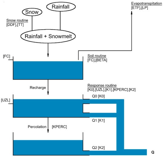
Figure 2.
HBV (Hydrologiska Byråns Vattenbalansavedelning) model structure (inspired by Bergström [38]). The model parameters are enclosed in square brackets.
2.5. Methodology
In this study, the HBV model sensitivity analysis was conducted using one of the most common approaches reported by Hamby [44] as “ONE-AT-A-TIME” (OAT) sensitivity measures. The latter consists of repeatedly varying one parameter at a time while keeping the rest fixed to their optimized values [44]. Furthermore, a bivariate analysis based on a “TWO-At-A-TIME” (TAT) version was used to highlight the interdependency of the model parameters. It has the same principle as the OAT approach except that two parameters are set to be varied instead of one parameter. Prior to both sensitivity and interdependency analysis, we evaluated the performance of the model to simulate the daily streamflow in the studied watershed. First of all, the initial values of the internal state variables of the model were retrieved using the first year (2001/2002) of the reference period for warm-up. Then, the model was calibrated/validated over each of the eight remaining years using a set of 1.5 million randomly generated parameter combinations (the parameter ranges are reported in Table 2). We adopted a cross-validation exercise, which involves using, iteratively, one year for calibration and each of the remaining years for validation.
Table 2.
HBV model parameter ranges used in calibration.
Long and consistent time series of meteorological variables are often hard to find worldwide, particularly over mountainous regions [55,62,63]. Numerous studies have evaluated the effect of the data length on model performance [64,65,66,67]. Theoretically, longer data series are expected to give steady optimal parameter estimates and consistent performance of conceptual hydrologic models. Various data lengths of three to eight years were recommended by different studies as sufficient for reliable model performance [64,65,67]. However, the nature of the data is more of a concern than its length according to numerous studies [42,68,69]. The efficient evaluation of a certain model requires that the data series contain all hydroclimatic conditions that may occur within the watershed of interest and not less than one year of length [42,66]. Gan et al. [70] found out that in some cases, one to two years could give better-performing models than ten years of calibration, as long as the data contain valuable information of the rainfall-runoff processes. The latter assures the adequate activation of the model parameters and avoids the misinterpretation of the model behavior and sensitivity. Moreover, numerous studies have pointed out that model parameters are time-variant and can be activated during different and short periods in time (e.g., [46,71]). This can be explained by the fact that different kinds of hydrological responses may occur within a short period, depending on rainfall intensities and antecedent wetness conditions [41]. Therefore, the changes in model parameters can be better captured when using shorter periods [72], particularly under unsteady hydroclimatic conditions.
The evaluation of the model outputs was carried out against daily observed streamflow using the Nash Sutcliff Efficiency (NSE) and the Root Mean Square Error (RMSE) metrics:
The NSE is firstly used as an objective function to select the most fitted model simulations to the observed streamflow. This statistical indicator is suggested as one of the most appropriate objective functions to provide reliable information about the overall model goodness of fit [73,74]. This suggestion is later endorsed by numerous studies related to hydrologic modeling [75,76]. A good model simulation involves the ability to reproduce the shape of the observed streamflow with the lowest bias possible. Legates and McCabe Jr. [73] recommended coupling multiple evaluation techniques for a more efficient model evaluation. This allows comprehensive performance assessment and accounts for both qualitative and quantitative aspects [74,76,77,78,79]. Thus, the RMSE was incorporated with the NSE to count for the bias between the observed and simulated streamflow.
The main problem related to the use of these metrics is associated with their difficult interpretation out of their range bounds (maximum and minimum values). Thus, a threshold beyond which the model performance can be judged as satisfactory remains hard to set. This issue was raised by many authors who discussed the suitability of available statistical indicators for computer model evaluation [73,79,80]. Besides, some authors proposed a classification of model performance as ratings to differentiate between poor and satisfactory simulations [75,76,81]. However, these classifications are case-specific and highly depend on model applications [75,82,83]. Moriasi et al. [75] conducted a review study related to computer model calibration/validation and proposed performance ratings for several statistical indicators. They suggested that model simulations with 0.5 < NSE ≤ 0.65 and NSE > 0.65 can be considered as satisfactory and having good performance, respectively. Furthermore, Singh et al. [81] recommended that an RMSE of 50% less than the standard deviation of the observed streamflow can be considered as low, while Moriasi et al. [75] considered this percentage as a reference for a very good model performance rating. Moreover, these ratings should present a certain flexibility based on the application the model is intended for, the quality of data, and the time step used for calibration [75]. For instance, higher evaluation metrics are needed for coarser time steps than for finer ones. Here, a model simulation is not considered as satisfactory unless the NSE is greater or equal to 0.5 and the corresponding RMSE is 30% less than the standard deviation of the observed streamflow.
3. Results and Discussion
3.1. Model Calibration and Validation
The model was run using data of eight consecutive hydrologic years from 2002/2003 to 2009/2010. The calibration exercise was carried out for each year separately. The statistics of simulations corresponding to NSEs above the 99.5th percentile (hereafter admissible simulations) and the streamflow simulations obtained based on the parameter sets that maximize the NSE during calibration are shown in Figure 3 and Figure 4, respectively. The resulted metrics suggest that, despite the scarcity of climatic data, the model is quite able to reproduce the daily streamflow observed at the outlet of the Ait Ouchene watershed. However, the performance accuracy is highly variable from one year to another, as shown in Figure 3. The model was found to provide the worst simulations in 2004/2005 and 2006/2007 years with maximum (minimum) NSE (RMSE) of 0.44 (3.62 m3/s) and 0.43 (4.14 m3/s), respectively. The low performance obtained in theses two years is largely due to the data quality. Both years presented a remarkable discrepancy between streamflow and rainfall in terms of event occurrence. From Figure 4 we note that there were instances where large amplitudes of streamflow were observed while no rainfall was recorded. This situation often characterizes regions with low-density networks, particularly those that receive local stormy events with smaller extents [84,85]. The performance was relatively higher for the years 2002/2003 and 2007/2008, as illustrated in Figure 3, with NSE (RMSE) values spanning between 0.46–0.79 (6.84 m3/s–10.20 m3/s) and 0.46–0.68 (3.70 m3/s–4.86 m3/s), respectively. The remaining years exhibited good agreement between the simulated and observed streamflow where all the NSE values were above 0.66 (2008/2009) and reached 0.90 (2005/2006), and all corresponding RMSE values were 30% below the standard deviation of the observed streamflow. Previous studies have reported that the calibration results are significantly affected by the changes in hydroclimatic conditions mainly driven by the strong spatiotemporal variability of rainfall [72,86]. The drier conditions are more problematic for conceptual models as they lead to the worst performance compared to humid conditions [64,67,72,86]. In the present study, the data series encompassed both drier and humid years without considering those with remarkable missed events (Table 1). The performance of the model during wet years agrees with the results from previous studies suggesting the easiness of model calibration during relatively wet conditions [36].
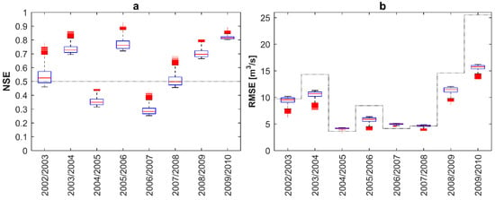
Figure 3.
NSE (a) and RMSE (b) statistical metrics corresponding to model simulations yielding Nash Sutcliff Efficiencies (NSEs) above the 99.5th percentile of the NSE values obtained during calibration. Each box shows minimum (bottom whisker), 25th percentile (bottom edge of the box), 50th percentile (red line inside the box), 75th percentile (top edge of the box), maximum (top whisker), and extreme values (red plus markers). The dashed lines correspond to the 0.5 NSE acceptance threshold (a) and the values of 30% less than the observed streamflow standard deviation (b).
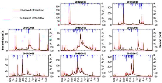
Figure 4.
Daily streamflow simulated using the annual optimal parameter combinations obtained during calibration.
Furthermore, the admissible simulations, obtained during calibration, from one year are verified in each of the remaining years. The summary of NSEs and RMSEs obtained after validation are illustrated in Table 3. The calibration and validation years are organized in columns and rows, respectively. As shown in Table 3, regardless of the calibration year, the model maintained the same level of low performance when validated in 2004/2005 and 2006/2007, with NSEs below the acceptance threshold. However, parameter combinations calibrated on the same years led to improved statistics when validated on other years. These results suggest that when relatively good quality data are available, the HBV model provides streamflow simulations that are fairly close to the observed streamflow at the outlet of the studied watershed. Furthermore, the model showed reasonable behavior during validation in years with reliable data. Still, we note that there were many instances where the performance of the model decreased rather than increased compared to the calibration runs. The change (decrease/increase) in the objective function mainly depends on the data used for calibration and validation [36,40,72,87]. The parameter combinations calibrated in 2002/2003 showed the largest NSE and RMSE drop-offs when they were validated in both 2005/2006 and 2008/2009. The drop-offs were less significant when the admissible simulations were verified against data of 2003/2004 and 2009/2010 (Table 3). Furthermore, 2002/2003 seemed to be the worst calibration/validation years. The parameter combinations calibrated in 2002/2003 were found to be less consistent in time compared to those calibrated in 2003/2004, 2005/2006, 2008/2009, or 2009/2010.
Table 3.
Maximum NSE and minimum Root Mean Square Error (RMSE) obtained after validation (calibration years in columns and validation years in rows).
Overall, it is widely known that under the inherent interaction between the conceptual model parameters, mainly driven by structure inadequacy [40,42], it is difficult to obtain a unique optimal set of parameters [39,42]. Multiple simulations that result in equally good performance exist [39,40]. Therefore, the parameter set that provided the best and consistent performance, according to both NSE and RMSE, was selected (Figure 5). This combination of parameters, not assumed as a realistic description of the physical processes controlling the hydrologic regime in the studied watershed, was used to investigate the sensitivity and interdependency of the model parameters.
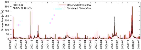
Figure 5.
Observed versus simulated daily streamflow using the parameter combinations yielding the best statistical metrics (NSE and RMSE) after validation.
3.2. Sensitivity Analysis
The sensitivity analysis was performed to quantify the individual effect of each parameter on the HBV model performance. This analysis was conducted by varying one parameter at a time while the rest are set to their optimized values. The degree of influence of each parameter was assessed according to the changes in the NSE objective function. The analysis covered six years of the reference period, where 2004/2005 and 2006/2007 years were excluded given the poor model performance driven by the low data quality. The sensitivity results are illustrated in Figure 6 where the changes in parameter values are plotted versus the changes in NSE values. It is clear from Figure 6 that there is an important year-to-year variability in the model behavior depending on the individual parameter changes. Generally, all parameters seemed to impact the model simulations to a certain extent. The latter depends on parameters and years. In our analysis, we observed that the parameter ETF demonstrated no major control over the model performance in most of the years. Except in 2008/2009, the increase in ETF parameter values led to the lowest NSEs. Overall, the model performed the best with smaller ETF values in all the considered years. Whereas, parameters such as DDF and LP seemed to have no effect on the model response in some years while they showed more influence in others. In most of these years, both parameters demonstrated overall NSE decreasing tendencies as the values of the parameters increased. In contrast, higher LP values in 2002/2003 resulted in higher NSEs, which means that the model performs the best under small evapotranspiration rates in such a year. The DDF was more dependent on the availability and extent of the snow cover over the study area. In previous studies, snowmelt related parameters, particularly DDF, were found to be more influential on the HBV model response in watersheds with a snow-dominated regime [40,47,88]. In contrast, the model performance had no clear dependency on the parameter in watersheds with rainfall dominated regimes due to the small snow portion in these watersheds [35,86]. Furthermore, when varied individually, the FC and BETA parameters seemed to have the most important impact on the model response. They presented the steepest curves in all the studied years. Numerous studies agreed that FC and BETA are one of the most influential parameters [35,40,46,47,72,88]. However, the parameter values that maximize the NSE change from one year to another. The FC, for instance, had optimal values within a range of 200 to more than 400 mm. It converged more towards the lower edge of the predefined calibration range in 2002/2003 and exceeded 400 mm in 2008/2009. The two years were contrasted in terms of hydroclimatic conditions. The first was marked as a relatively dry year with unevenly distributed rainfall events, one of which caused an extremely high peak flow (Figure 4), while the second was a very wet year with relatively high annual rainfall amount and above-average snow cover (Table 1). Theoretically, the FC parameter determines the amount of excess water contributing to the upper reservoir recharge. A lower FC, which refers to a soil layer with less water holding capacity, would amplify the portion of excess water compared to larger FC values. Merz et al. [86] and Osuch et al. [72] showed that FC positively correlates with precipitation but more significantly with temperature. However, the parameter presents different behaviors in different watersheds depending on the presence or absence of snow cover [72]. It tends to increase with temperature in snow-covered watersheds while it shows the opposite tendency in watersheds without snow cover. The findings of Merz et al. [86] and Osuch et al. [72] would suggest that the positive correlation between FC and temperature in snow-covered watersheds may be related to increasing snowmelt supplies to the soil subroutine. The latter partly explains the variability in FC optima in our case, where it tended to be larger in years characterized by relatively important snow cover (2005/2006 and 2008/2009). This observation suggests that the FC optima fluctuations are subject to changes in the total water supply, particularly from snowmelt. This interpretation agrees with the finding from Abebe et al. [46], where the FC was found to take lower values during dry periods and high values during wet periods with susceptible overestimated rainfall. Contrary to FC, the annual optimal values of BETA varied within a narrower section of its predefined range throughout the reference period. This may be explained by the adjustment of BETA to the FC optimal values in order to counterbalance the water supply offset provoked by a larger water holding capacity. As shown in Figure 5, the parameter combination obtained after validation often led the model to underestimate high peak flows. The latter would require smaller FCs in order to be correctly simulated. Hence, the bias provoked by the relatively higher optimized FC is accounted for by BETAs that are smaller than those obtained after validation (Figure 6). The smaller BETA values, which mean more recharge water towards the upper reservoir, resulted in higher NSEs, particularly in 2002/2003 and 2003/2004. Moreover, the parameters KPERC and UZL, which control the drainage of the upper reservoir, showed relatively similar behavior to the FC in both 2002/2003 and 2008/2009. As can be seen in Figure 6, in 2002/2003, higher NSEs were obtained by small KPERC and small UZL values, while the opposite was true in 2008/2009. Additionally, the K0 intervened only when the conditions were wet enough to allow the exceedance of the UZL, otherwise, the simulated outflow was mainly the result of the K1 contribution. Generally, a smaller UZL allowed more contribution from the K0 in peak flows generation. This can be seen in the subplots relative to K0 and K1 in Figure 6. Particularly during 2005/2006 and 2007/2008, K0 induced no change in the objective function when varied over its whole range. The K1, in contrast, resulted in steeper curves suggesting a significant control over the model response. The effect of the K0 parameter can be also seen when there was a relatively large water supply from individual rainfall events resulting in important peak flows [46,89], such as the case of 2002/2003 and 2003/2004. Such peak flows are often driven by extremely intense rainfall events that produce important runoff in a short amount of time. Additionally, the K2 which is responsible for baseflow generation presented a certain degree of influence on the global flow generation. However, the model sensitivity to K2 highly depends on the simultaneous effect of K1 and KPERC on the water level in the upper reservoir [39,40]. In the present study, the larger optimized KPERC was the main factor that led to the significant contribution of K2 in the global outflow.
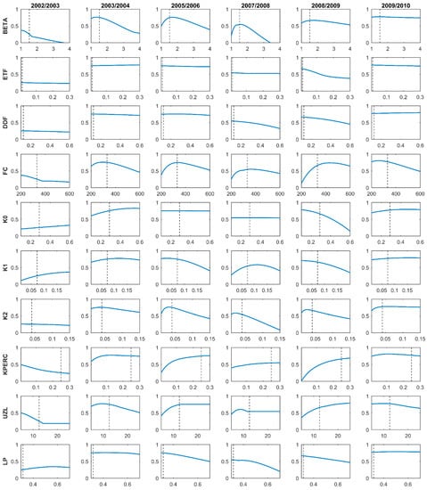
Figure 6.
The sensitivity of the model to the changes in parameter values according to the NSE. The dashed lines represent the optimal parameter values obtained after validation.
3.3. Parameters Interdependency
Generally, model parameters, as physical as they sound, may not reasonably describe the reality of the physical processes [88,90], particularly with conceptual models that are highly subject to parameter interdependency. In the present study, we were able to highlight the potential interdependency of the model parameters through the sensitivity analysis. The findings suggest that the change in one of the model parameters due to hydroclimatic conditions, for instance, would be offset by one or more of the remaining parameters to provide the most fitted model to the observed streamflow. This combining effect is responsible to a large extent for the year-to-year variability of the estimated optimal model parameters [66]. To emphasize the interdependency of the HBV model parameters, a bivariate analysis based on the NSE criterion was carried out. It consisted of varying two parameters at a time over their whole predefined range instead of one parameter, while the rest were set to their optimal values obtained after validation. Figure 7 shows the maximum NSE obtained for each couple of parameters, where the diagonal cells of each subplot represent the maximum NSE from the OAT analysis. Previous studies have demonstrated that the use of fewer parameters than the full version has little impact on the model fit [47,90]. Our results show that combining a minimum of two parameters, while the rest are set to their optimized values, leads to NSEs comparable to those obtained during calibration. Still, the couple that yields to the best fit highly depends on the year during which the model is run. Overall, less influential parameters, such as ETF, LP, and DDF, when they were combined brought no significant change compared to the OAT analysis, as shown in Figure 7. However, the incorporation of other parameters, with more influence on the model response, in the parameter couple resulted in higher NSEs. The most significant increases were obtained when one or more of the response routine parameters were considered. This remark holds true for all the studied years unless the conditions were not met to allow the engagement of some of the parameters, such as UZL in 2005/2006 and K0 in 2007/2008 hydrologic years. Overall, the results from all the years lead us to conclude that the combination of the response routine parameters, particularly K0, KPERC, and UZL, yield superior model simulations. Thus, the overall performance of the model would be more sensitive to the response routine parameters than to those of the soil moisture routine, particularly in years with extremely high peak flows. The impact of the response routine on the model performance was obvious in 2002/2003. As shown in Figure 7, the parameter couples constituted either of UZL or KPERC returning the highest NSEs, especially when combined with K0. Furthermore, in years with frequent snow cover (2005/2006 and 2008/2009, Table 1) the couple FC-DDF seemed to result in NSEs as high as those obtained by the response routine parameters.
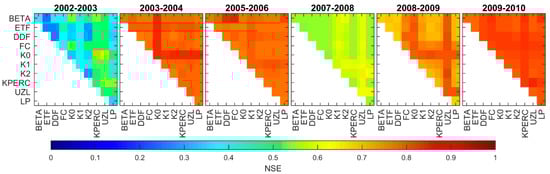
Figure 7.
Heatmaps representing the maximum NSE obtained when varying two model parameters at a time while the rest are set to their optimized values.
The interaction between the values of the five parameter couples (FC-DDF, FC-K0, FC-KPERC, K0-KPERC, and K0-UZL) that caused an overall distinct increase in the NSE values, as shown in Figure 7, was further investigated. Figure 8 illustrates the scatter plots of the five parameter couples classified according to the NSE resulted from the combination of each pair of parameter values. Each row represents the results of one parameter couple in four representative years (2002/2003, 2003/2004, 2005/2006, and 2008/2009). Figure 8 confirms that FC was strongly influenced by the year-to-year changes in water supplies. Remarkably, the parameter positively correlated with the yearly snow cover anomaly. Moreover, it seemed to change according to the changes in DDF. As shown in Figure 8, when FC and DDF were varied together, in years with frequent snow cover (2005/2006 and 2008/2009), we observed that both parameters took higher values to yield the best NSEs. This suggests that important amounts of snowmelt produced under higher DDFs are compensated with higher FCs. In contrast, when varied with other parameters, such as KPERC and K0, the FC significantly decreased, yet the maximal NSE did not change as much. This observation suggests that the higher FC values in both years may be set to counterbalance a potentially overestimated snowmelt. This is in line with the interpretation of Abebe et al. [46] assuming that the parameter takes higher values to reduce the effect of overestimated rainfall. Furthermore, from the scatter plots, we can see that the five considered couples presented contrasting behavior in 2002/2003 and 2008/2009. There was a general tendency where the set of parameter pairs that yield the maximum NSEs, regardless of the actual values, were always on the opposite sides of the parameter ranges. In 2002/2003, the best simulations were the result of the couples that incorporated DDF, FC, KPERC, and UZL parameter values around the lower edge of their predefined range, and larger K0. Conversely, larger values from DDF, FC, KPERC, and UZL, and smaller K0 values provided the best simulations in 2008/2009. The small FC values allowed the small discrete rainfall amounts, in 2002/2003, to fully participate in the upper reservoir recharge. Accordingly, the response subroutine parameters were set in a way to reduce the potential storage of the upper reservoir and percolation rate so that the smaller recharge supplies could significantly contribute to the global outflow. A reverse behavior was observed in 2008/2009. In other words, the combination of the same parameters provoked an enlargement of the upper reservoir storage capacity, which led to a reduction in the excess water from the reservoir. On the one hand, these observations suggest that in addition to FC, all the parameters engaged in the drainage of the upper reservoir compensate for the bias that may take place from an overestimated water supply. On the other hand, under high peak flows, the same parameters are combined to enhance the contribution of small water supplies to the global outflow. In particular, the reduction in the upper reservoir storage capacity may be considered as a mimic of the rapid saturation of the upper soil layer under intense rainfall events, which was the case in 2002/2003 and 2003/2004. Although limited to FC, a similar observation was made by Abebe et al. [46]. They explained the changes in the optimal FC values by the absence of model formulations that account for factors controlling the infiltration-runoff partitioning, such as rainfall intensity and duration.
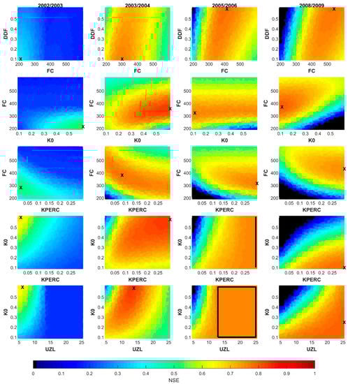
Figure 8.
Scatter plots of the five parameter couples FC-DD, FC-K0, FC-KP, K0-KP, and K0-UZL classified according to the NSE values. The X marker refers to the best-performing pair of parameter values. The continuous black lines enclose the combinations of parameter values that result in the same NSE values.
4. Conclusions
The present study was performed to investigate the potential influence of the HBV model parameters on the streamflow simulation over a semi-arid watershed characterized by heterogenous hydroclimatic conditions. The analysis was conducted using a set of nine years of hydroclimatic measurements and remotely sensed snow cover data, where the first year of the reference period was used for model warm-up. The model performance was firstly tested through a cross-validation exercise. Then, the best performing combination of parameters was chosen to investigate the sensitivity and parameter interdependency using the “ONE-AT-A-TIME” and “TWO-AT-A-TIME” analysis, respectively.
Our results show that the HBV model can fairly reproduce the daily streamflow at the outlet of the studied watershed. The statistical metrics obtained during calibration present a significant variability from one year to another. The worst model performance was obtained in relatively dry years. The performance was relatively higher in the remaining years with good agreements between simulated and observed streamflow. The results of the sensitivity analysis indicated that each of the model parameters influences the simulated streamflow to a certain extent. However, the degree of influence depends on parameters and years. We found that the parameter ETF has no major influence on the model performance in most of the years. The model was found to be more sensitive to FC and BETA parameters. Furthermore, we observed that the optimal parameters present significant annual variability driven by the changes in hydroclimatic conditions. It was found that, during years with extremely high peak flows, the soil routine parameters assume values that lead to the amplification of the amount of water drained towards the upper reservoir. Meanwhile, the upper reservoir related parameters (UZL, K0, and KPERC) combine to reduce its storage capacity to ensure important excess water from smaller amounts of water supplies. The same parameters were found to present a reverse behavior in years with abundant snow cover. Particularly, the FC showed higher sensitivity to the total water supply, mainly to the overestimated snowmelt produced under abundant snow cover.
In summary, the results of our analyses in the present study highlight the main challenges associated with hydrological modeling studies in our context, especially the high interdependency between model parameters and the strong impact of changes in hydroclimatic conditions. However, despite the lack of efficient ground datasets, the relatively good streamflow simulations obtained using the HBV model at daily time steps are very promising. Deeper knowledge about the runoff-infiltration partitioning and the nature of the snowmelt contribution to the streamflow in this region should be characterized to support the findings of this study.
Author Contributions
Study conceptualization, H.O. and A.B. (Abdelghani Boudhar); Data processing and modelling tasks, H.O.; analysis and result interpretation, H.O. and A.B. (Abdelghani Boudhar); writing—original draft preparation, H.O; writing—review and editing, A.B. (Abdelghani Boudhar), A.O., A.B. (Abdelaziz Beljadid), M.L., and A.C. All authors have read and agreed to the published version of the manuscript.
Funding
This research received no external funding.
Acknowledgments
A.B. (Abdelghani Boudhar) and A.C are supported by the research program “MorSnow-1”, International Water Research Institute (IWRI), Mohammed VI Polytechnic University (UM6P), Morocco, (Accord spécifique n° 39 entre OCP S.A et UM6P). We thank the Oum Er-Rbia Hydraulic Basin Agency for providing the observed data used in this study. We thank the anonymous reviewers for their helpful and constructive review.
Conflicts of Interest
The authors declare no conflict of interest.
References
- Bergström, S.; Lindström, G. Interpretation of runoff processes in hydrological modelling-experience from the HBV approach. Hydrol. Process. 2015, 29, 3535–3545. [Google Scholar] [CrossRef]
- Rango, A.; Martinec, J. Application of a Snowmelt-Runoff Model Using Landsat Data. Nord. Hydrol. 1979, 10, 225–238. [Google Scholar] [CrossRef]
- Vandewiele, G.L.; Xu, C.Y. Ni-Lar-Win Methodology and comparative study of monthly water balance models in Belgium, China and Burma. J. Hydrol. 1992, 134, 315–347. [Google Scholar] [CrossRef]
- Zhao, R.J. The Xinanjiang model applied in China. J. Hydrol. 1992, 135, 371–381. [Google Scholar]
- Todini, E. The ARNO rainfall-runoff model. J. Hydrol. 1996, 175, 339–382. [Google Scholar] [CrossRef]
- Arnold, J.G.; Fohrer, N. SWAT2000: Current capabilities and research opportunities in applied watershed modelling. Hydrol. Process. 2005, 19, 563–572. [Google Scholar] [CrossRef]
- Liang, X.; Lettenmaier, D.P.; Wood, E.F.; Burges, S.J. A simple hydrologically based model of land surface water and energy fluxes for general circulation model. J. Geophys. Res. 1994, 99, 14415–14428. [Google Scholar] [CrossRef]
- Bergström, S.; Forsman, A. Development of a Conceptual Deterministic Rainfall-Runoff Model. Nord. Hydrol. 1973, 4, 147–170. [Google Scholar] [CrossRef]
- Orth, R.; Staudinger, M.; Seneviratne, S.I.; Seibert, J.; Zappa, M. Does model performance improve with complexity? A case study with three hydrological models. J. Hydrol. 2015, 523, 147–159. [Google Scholar] [CrossRef]
- Beven, K. Changing ideas in hydrology—The case of physically based models. J. Hydrol. 1989, 105, 157–172. [Google Scholar] [CrossRef]
- Bergström, S. Experience from Applications of the HBV Hydrological Model from the Perspective of Prediction in Ungauged Basins; MOPEX Experiments; IAHS Publ.: Wallingford, UK, 2006; Volume 307. [Google Scholar]
- Abulohom, M.S.; Shah, S.M.S.; Ghumman, A.R. Development of a Rainfall-Runoff Model, its Calibration and Validation. Water Resour. Manag. 2001, 15, 149–163. [Google Scholar] [CrossRef]
- WMO. Intercomparison of Conceptual Models Used in Operational Hydrological Forecasting; WMO: Geneva, Switzerland, 1975. [Google Scholar]
- WMO. Intercomparison of Models of Snowmelt Runoff; WMO: Geneva, Switzerland, 1986. [Google Scholar]
- Abdulla, F.; Al-Badranih, L. Application of a rainfall-runoff model to three catchments in Iraq. Hydrol. Sci. J. 2010, 45, 13–25. [Google Scholar] [CrossRef]
- Beven, K.; Freer, J. Equifinality, data assimilation, and uncertainty estimation in mechanistic modelling of complex environmental systems using the GLUE methodology. J. Hydrol. 2001, 249, 11–29. [Google Scholar] [CrossRef]
- Braun, J.N.; Renner, C.B. Application of a conceptual runoff model in different physiographic regions of Switzerland. Hydrol. Sci. J. 1992, 37, 217–231. [Google Scholar] [CrossRef]
- Seibert, J. HBV Light Version 2 User’s Manual; Stockholm University, Department of Physical Geography and Quaternary Geology: Stockholm, Sweden, 2005. [Google Scholar]
- Stahl, K.; Moore, R.D.; Shea, J.M.; Hutchinson, D.; Cannon, A.J. Coupled modelling of glacier and streamflow response to future climate scenarios. Water Resour. Res. 2008, 44, 1–13. [Google Scholar] [CrossRef]
- Krysanova, V.; Bronstert, A.; Müller-wohlfeil, D.-I. Modelling river discharge for large drainage basins: From lumped to distributed approach. Hydrol. Sci. J. 1999, 44, 313–331. [Google Scholar] [CrossRef]
- Lindström, G.; Johansson, B.; Persson, M.; Gardelin, M.; Bergström, S. Development and test of the distributed HBV-96 hydrological model. J. Hydrol. 1997, 201, 272–288. [Google Scholar] [CrossRef]
- Rientjes, T.H.M.; Muthuwatta, L.P.; Bos, M.G.; Booij, M.J.; Bhatti, H.A. Multi-variable calibration of a semi-distributed hydrological model using streamflow data and satellite-based evapotranspiration. J. Hydrol. 2013, 505, 276–290. [Google Scholar] [CrossRef]
- Thapa, B.R.; Ishidaira, H.; Pandey, V.P.; Shakya, N.M. A multi-model approach for analyzing water balance dynamics in Kathmandu Valley, Nepal. J. Hydrol. Reg. Stud. 2017, 9, 149–162. [Google Scholar] [CrossRef]
- Vehviläinen, B.; Lohvansuu, J. The effects of climate change on discharges and snow cover in Finland. Hydrol. Sci. J. 1991, 36, 109–121. [Google Scholar] [CrossRef]
- Saelthun, N.R.; Aittoniemi, P.; Bergström, S. Climate Change Impacts on Runoff and Hydropower in the Nordic Countries Final Report from the Project “Climate Change and Energy Production”; Nordic Council of Ministers: Kobenhavn, Denmark, 1998. [Google Scholar]
- Bergström, S.; Carlsson, B.; Gardelin, M.; Lindström, G.; Petterson, A.; Rummukainen, M. Climate change impacts on runoff in Sweden—Assessments by global climate models, dynamical downscalling and hydrological modelling. Clim. Res. 2001, 16, 101–112. [Google Scholar] [CrossRef]
- Chen, H.; Xiang, T.; Zhou, X. Impacts of climate change on the Qingjiang Watershed ’ s runoff change trend in China. Stoch. Environ. Res. Risk Assess. 2012, 26, 847–858. [Google Scholar] [CrossRef]
- Brandt, M.; Bergström, S.; Gardelin, M. Modelling the effects of clearcutting on runoff—Examples from central Sweden. Ambio 1988, 17, 307–313. [Google Scholar]
- Teutschbein, C.; Grabs, T.; Laudon, H.; Karlsen, R.H.; Bishop, K. Simulating streamflow in ungauged basins under a changing climate: The importance of landscape characteristics. J. Hydrol. 2018, 561, 160–178. [Google Scholar] [CrossRef]
- Parra, V.; Arumí, J.L.; Muñoz, E. Identifying a Suitable Model for Low-Flow Simulation in Watersheds of South-Central Chile: A Study Based on a Sensitivity Analysis. Water 2019, 11, 1506. [Google Scholar] [CrossRef]
- Johansson, B. Runoff calculations in ungauged catchments—An evaluation of the Pulse model. Vatten 1992, 48, 111–116. [Google Scholar]
- Arheimer, B. Evaluation of water quantity and quality modelling in ungauged European basins. In Predictions in Ungauged Basins: Promise and Progress; IAHS Publ. No. 303: Foz do Iguaçu, Brazil, 2006; pp. 99–107. [Google Scholar]
- Samuel, J.; Coulibaly, P.; Metcalfe, R.A. Identification of rainfall-runoff model for improved baseflow estimation in ungauged basins. Hydrol. Process. 2012, 26, 356–366. [Google Scholar] [CrossRef]
- Seibert, J.; Beven, K.J. Gauging the ungauged basin: How many discharge measurements are needed? Hydrol. Earth Syst. Sci. 2009, 13, 883–892. [Google Scholar] [CrossRef]
- Parra, V.; Fuentes-Aguilera, P.; Muñoz, E. Identifying advantages and drawbacks of two hydrological models based on a sensitivity analysis: A study in two Chilean watersheds. Hydrol. Sci. J. 2018, 63, 1831–1843. [Google Scholar] [CrossRef]
- Dakhlaoui, H.; Ruelland, D.; Tramblay, Y.; Bargaoui, Z. Evaluating the robustness of conceptual rainfall-runoff models under climate variability in northern Tunisia. J. Hydrol. 2017, 550, 201–217. [Google Scholar] [CrossRef]
- Poméon, T.; Jackisch, D.; Diekkrüger, B. Evaluating the performance of remotely sensed and reanalysed precipitation data over West Africa using HBV light. J. Hydrol. 2017, 547, 222–235. [Google Scholar] [CrossRef]
- Bergström, S. The HBV Model—Its Structure and Applications; Swedish Meteorological and Hydrological Institute: Norrköping, Sweden, 1992. [Google Scholar]
- Uhlenbrook, S.; Seibert, J.; Leibundgut, C.; Rodhe, A. Prediction uncertainty of conceptual rainfall- runoff models caused by problems in identifying model parameters and structure. Hydrol. Sci. J. 1999, 44, 779–797. [Google Scholar] [CrossRef]
- Seibert, J. Estimation of parameter uncertainty in the HBV model. Nord. Hydrol. 1997, 28, 247–262. [Google Scholar] [CrossRef]
- Keith, B.; Andrew, B. The future of distributed models: Model calibration and uncertainty prediction. Hydrol. Process. 1992, 6, 279–298. [Google Scholar]
- Sorooshian, S.; Gupta, V.K. Automatic calibration of conceptual rainfall-runoff models: The question of parameter observability and uniqueness. Water Resour. Res. 1983, 19, 260–268. [Google Scholar] [CrossRef]
- Gan, T.Y.; Biftu, G.F. Automatic calibration of conceptual rainfall-runoff models: Optimization algorithms, catchment conditions and model structure. Water Resour. Res. 1996, 32, 3513–3524. [Google Scholar] [CrossRef]
- Hamby, D.M. A review of techniques for parameter sensitivity analysis of environmental models. Environ. Monit. Assess. 1994, 32, 135–154. [Google Scholar] [CrossRef]
- McCuen, R.H. The role of sensitivity analysis in hydrologic modeling. J. Hydrol. 1973, 18, 37–53. [Google Scholar] [CrossRef]
- Abebe, N.A.; Ogden, F.L.; Pradhan, N.R. Sensitivity and uncertainty analysis of the conceptual HBV rainfall-runoff model: Implications for parameter estimation. J. Hydrol. 2010, 389, 301–310. [Google Scholar] [CrossRef]
- Zelelew, M.B.; Alfredsen, K. Sensitivity-guided evaluation of the HBV hydrological model parameterization. J. Hydroinform. 2013, 15, 967–990. [Google Scholar] [CrossRef]
- Herman, J.D.; Reed, P.M.; Wagener, T. Time-varying sensitivity analysis clarifies the effects of watershed model formulation on model behavior. Water Resour. Res. 2013, 49, 1400–1414. [Google Scholar] [CrossRef]
- El Azhari, M.; Loudyi, D. Analysis of the Water-Energy nexus in central Oum Er-Rbia sub-basin—Morocco. Int. J. River Basin Manag. 2019, 17, 13–24. [Google Scholar] [CrossRef]
- Ouatiki, H.; Boudhar, A.; Tramblay, Y.; Jarlan, L.; Benabdelouhab, T.; Hanich, L.; El Meslouhi, M.; Chehbouni, A. Evaluation of TRMM 3B42 V7 Rainfall Product over the Oum Er Rbia Watershed in Morocco. Climate 2017, 5, 1. [Google Scholar] [CrossRef]
- Lebrini, Y.; Boudhar, A.; Hadria, R.; Lionboui, H.; Elmansouri, L.; Arrach, R.; Ceccato, P.; Benabdelouahab, T. Identifying Agricultural Systems Using SVM Classification Approach Based on Phenological Metrics in a Semi-arid Region of Morocco. Earth Syst. Environ. 2019, 3, 277–288. [Google Scholar] [CrossRef]
- Htitiou, A.; Boudhar, A.; Lebrini, Y.; Hadria, R.; Lionboui, H.; Elmansouri, L.; Tychon, B.; Benabdelouahab, T. The Performance of Random Forest Classification Based on Phenological Metrics Derived from Sentinel-2 and Landsat 8 to Map Crop Cover in an Irrigated Semi-arid Region. Remote Sens. Earth Syst. Sci. 2019, 2, 208–224. [Google Scholar] [CrossRef]
- Ouatiki, H.; Boudhar, A.; Ouhinou, A.; Arioua, A.; Hssaisoune, M.; Bouamri, H.; Benabdelouahab, T. Trend analysis of rainfall and drought over the Oum Er-Rbia River Basin in Morocco during 1970–2010. Arab. J. Geosci. 2019, 12, 128. [Google Scholar] [CrossRef]
- Boudhar, A.; Ouatiki, H.; Bouamri, H.; Lebrini, Y.; Karaoui, I.; Hssaisoune, M.; Arioua, A.; Benabdelouahab, T. Hydrological Response to Snow Cover Changes Using Remote Sensing over the Oum Er Rbia Upstream Basin, Morocco. In Mapping and Spatial Analysis of Socio-Economic and Environmental Indicators for Sustainable Development; Rebai, N., Mastere, M., Eds.; Springe Cham: Cham, Switzerland, 2020; pp. 95–102. [Google Scholar]
- Boudhar, A.; Hanich, L.; Boulet, G.; Duchemin, B.; Berjamy, B.; Chehbouni, A. Evaluation of the Snowmelt Runoff model in the Moroccan High Atlas Mountains using two snow-cover estimates. Hydrol. Sci. J. 2009, 54, 1094–1113. [Google Scholar] [CrossRef]
- Thornthwaite, C.W. An Approach toward a Rational. Geogr. Rev. 1948, 38, 55–94. [Google Scholar] [CrossRef]
- Hall, D.K.; Riggs, G.A. MODIS/Terra Snow Cover Daily L3 Global 500m SIN Grid, Version 6. [h17v5]; NASA National Snow and Ice Data Center Distributed Active Archive Center: Boulder, CO, USA, 2016. [Google Scholar]
- Marchane, A.; Jarlan, L.; Hanich, L.; Boudhar, A.; Gascoin, S.; Tavernier, A.; Filali, N.; Page, M.L.; Hagolle, O.; Berjamy, B. Assessment of daily MODIS snow cover products to monitor snow cover dynamics over the Moroccan Atlas mountain range. Remote Sens. Environ. 2015, 160, 72–86. [Google Scholar] [CrossRef]
- Lee, S.; Klein, A.G.; Over, T.M. A comparison of MODIS and NOHRSC snow-cover products for simulating streamflow using the Snowmelt Runoff Model. Hydrol. Process. 2005, 19, 2951–2972. [Google Scholar] [CrossRef]
- Li, X.; Williams, M.W. Snowmelt runoff modelling in an arid mountain watershed, Tarim Basin, China. Hydrol. Process. 2008, 22, 3931–3940. [Google Scholar] [CrossRef]
- Sorman, A.A.; Sensoy, A.; Tekeli, A.E.; Sorman, A.Ü.; Akyurek, Z. Modelling and forecasting snowmelt runoff process using the HBV model in the eastern part of Turkey. Hydrol. Process. 2009, 23, 1031–1040. [Google Scholar] [CrossRef]
- Boudhar, A.; Boulet, G.; Hanich, L.; Sicart, J.E.; Chehbouni, A. Energy fluxes and melt rate of a seasonal snow cover in the Moroccan High Atlas. Hydrol. Sci. J. 2016, 61, 931–943. [Google Scholar] [CrossRef]
- Baba, M.W.; Gascoin, S.; Jarlan, L.; Simonneaux, V.; Hanich, L. Variations of the snow water equivalent in the ourika catchment (Morocco) over 2000–2018 using downscaled MERRA-2 data. Water 2018, 10, 1120. [Google Scholar] [CrossRef]
- Li, C.Z.; Wang, H.; Liu, J.; Yan, D.H.; Yu, F.L.; Zhang, L. Effect of calibration data series length on performance and optimal parameters of hydrological model. Water Sci. Eng. 2010, 3, 378–393. [Google Scholar]
- Xia, Y.; Yang, Z.-L.; Jackson, C.; Stoffa, P.L.; Sen, M.K. Impacts of data length on optimal parameter and uncertainty estimation of a land surface model. J. Geophys. Res. 2004, 109, 1–13. [Google Scholar] [CrossRef]
- Sorooshian, S. Evaluation of Maximum Likelihood Parameter Estimation Techniques for and Length on Model Credibility. Water Resour. Res. 1983, 19, 251–259. [Google Scholar] [CrossRef]
- Anctil, F.; Perrin, C.; Andréassian, V. Impact of the length of observed records on the performance of ANN and of conceptual parsimonious rainfall-runoff forecasting models. Environ. Model. Softw. 2004, 19, 357–368. [Google Scholar] [CrossRef]
- Viviroli, D.; Zappa, M.; Schwanbeck, J.; Gurtz, J.; Weingartner, R. Continuous simulation for flood estimation in ungauged mesoscale catchments of Switzerland—Part I: Modelling framework and calibration results. J. Hydrol. 2009, 377, 191–207. [Google Scholar] [CrossRef]
- Jain, S.K. Calibration of conceptual models for rainfall-runoff simulation. Hydrol. Sci. J. 1993, 38, 431–441. [Google Scholar] [CrossRef]
- Gan, T.Y.; Dlamini, E.M.; Biftu, G.F. Effects of model complexity and structure, data quality, and objective functions on hydrologic modeling. J. Hydrol. 1997, 192, 81–103. [Google Scholar] [CrossRef]
- Tripp, D.R.; Niemann, J.D. Evaluating the parameter identifiability and structural validity of a probability-distributed model for soil moisture. J. Hydrol. 2008, 353, 93–108. [Google Scholar] [CrossRef]
- Osuch, M.; Romanowicz, R.J.; Booij, M.J. The influence of parametric uncertainty on the relationships between HBV model parameters and climatic characteristics. Hydrol. Sci. J. 2015, 60, 1299–1316. [Google Scholar] [CrossRef]
- Legates, D.R.; McCabe, G.J., Jr. Evaluating the use of “Goodness of Fit” measures in hydrologic and hydroclimatic model validation. Water Resour. Res. 1999, 35, 233–241. [Google Scholar] [CrossRef]
- Willmott, C.J. On the validation of models. Phys. Geogr. 2013, 2, 37–41. [Google Scholar] [CrossRef]
- Moriasi, D.N.; Arnold, J.G.; Van Liew, M.W.; Bingner, R.L.; Harmel, R.D.; Veith, T.L. Model evaluation guidelines for systematic quantification of accuracy in watershed simulations. Am. Soc. Agric. Biol. Eng. 2007, 50, 885–900. [Google Scholar]
- Ritter, A.; Muñoz-carpena, R. Performance evaluation of hydrological models: Statistical significance for reducing subjectivity in goodness-of-fit assessments. J. Hydrol. 2013, 480, 33–45. [Google Scholar] [CrossRef]
- Biondi, D.; Freni, G.; Iacobellis, V.; Mascaro, G.; Montanari, A. Validation of hydrological models: Conceptual basis, methodological approaches and a proposal for a code of practice. Phys. Chem. Earth 2012, 42, 70–76. [Google Scholar] [CrossRef]
- Pushpalatha, R.; Perrin, C.; Le, N.; Andréassian, V. A review of efficiency criteria suitable for evaluating low-flow simulations. J. Hydrol. 2012, 420, 171–182. [Google Scholar] [CrossRef]
- Willmott, C.J.; Ackleson, S.G.; Davis, R.E.; Feddema, J.J.; Klink, K.M.; Legates, D.R.; O’Donnell, J.; Rowe, C.M. Statistics for the evaluation and comparison of models. J. Geophys. Res. 1985, 90, 8995–9005. [Google Scholar] [CrossRef]
- Garrick, M.; Cunnane, C.; Nash, J.E. A criterion of efficiency for rainfall-runoff models. J. Hydrol. 1978, 36, 375–381. [Google Scholar] [CrossRef]
- Singh, J.; Knapp, H.V.; Demissie, M. Hydrologic Modeling of the Iroquois River Watershed Using HSPF and SWAT. J. Am. Water Resour. Assoc. 2005, 41, 343–360. [Google Scholar] [CrossRef]
- Beven, K. A manifesto for the equifinality thesis. J. Hydrol. 2006, 320, 18–36. [Google Scholar] [CrossRef]
- Klemeš, V. Operational testing of hydrological simulation models. Hydrol. Sci. J. 1986, 31, 13–24. [Google Scholar] [CrossRef]
- Xu, H.; Xu, C.; Chen, H.; Zhang, Z.; Li, L. Assessing the influence of rain gauge density and distribution on hydrological model performance in a humid region of China Hongliang. J. Hydrol. 2013, 505, 1–12. [Google Scholar] [CrossRef]
- Dong, X.; Dohmen-Janssen, C.M.; Booij, M.J. Appropriate spatial sampling of rainfall for flow simulation. Hydrol. Sci. J. 2005, 50, 279–297. [Google Scholar] [CrossRef]
- Merz, R.; Parajka, J.; Blöschl, G. Time stability of catchment model parameters: Implications for climate impact analyses. Water Resour. Res. 2011, 47, 1–17. [Google Scholar] [CrossRef]
- Coron, L.; Andréassian, V.; Perrin, C.; Lerat, J.; Vaze, J.; Bourqui, M.; Hendrickx, F. Crash testing hydrological models in contrasted climate conditions: An experiment on 216 Australian catchments. Water Resour. Res. 2012, 48, 1–17. [Google Scholar] [CrossRef]
- Uhlenbrook, S.; Holocher, J.; Leibundgut, C.; Seibert, J. Using a conceptual rainfall-runoff model on different scales by comparing a headwater with larger basins. In Hydrology, Water Resources and Ecology in Headwaters; IAHS Publ. No. 248: Meran, Italy, 1998; pp. 297–305. [Google Scholar]
- Ouyang, S.; Puhlmann, H.; Wang, S.; von Wilpert, K.; Sun, O.J. Parameter uncertainty and identifiability of a conceptual semi-distributed model to simulate hydrological processes in a small headwater catchment in Northwest China. Ecol. Process. 2014, 3, 1–14. [Google Scholar] [CrossRef]
- Seibert, J. Regionalisation of parameters for a conceptual rainfall-runoff model. Agric. For. Meteorol. 1999, 98, 279–293. [Google Scholar] [CrossRef]


© 2020 by the authors. Licensee MDPI, Basel, Switzerland. This article is an open access article distributed under the terms and conditions of the Creative Commons Attribution (CC BY) license (http://creativecommons.org/licenses/by/4.0/).