Abstract
Water scarcity is a key challenge to global development. In Brazil, the Sao Francisco River Basin (SFB) has experienced water scarcity problems because of decreasing streamflow and increasing demands from multiple sectors. However, the drivers of decreased streamflow, particularly the potential role of the surface-groundwater interaction, have not yet been investigated. Here, we assess long-term trends in the streamflow and baseflow of the SFB during 1980–2015 and constrain the most likely drivers of observed decreases through a trend analysis of precipitation (P), evapotranspiration (ET), and terrestrial water storage change (TWS). We found that, on average, over 86% of the observed decrease in streamflow can be attributed to a significant decreasing baseflow trend along the SFR, with a spatial agreement between the decreased baseflow, increased ET, and irrigated agricultural land in the Middle SFB. We also noted a decreasing trend in TWS across the SFB exceeding –20 mm year−1. Overall, our findings indicate that decreasing groundwater contributions (i.e., baseflow) are providing the observed reduction in the total SFR flow. A lack of significant P trends and the strong TWS depletion indicate that a P variability only has likely not caused the observed baseflow reduction, in mainly the Middle and Sub-middle SFB. Therefore, groundwater and surface withdrawals may likely be a driver of baseflow reduction in some regions of the SFB.
1. Introduction
The World Economic Forum has categorized water crises as one of the top-ranked global (severe) risks since 2012 [1], and water is increasingly becoming a priority policy issue at global scales [2]. Ensuring global access to freshwater is one of the United Nations Sustainable Development Goals (SDGs) addressed in the 2030 Agenda [3]. To fulfill the 2030 Agenda, decision makers face the complex challenge of balancing water resource availability and water demands [2,4]. Unfortunately, the imbalance between water supply and demand has led to water scarcity [5]. In fact, there is an increasing trend in water scarcity worldwide [6], triggered in many locations by the increase of anthropogenic water use [7].
Streamflow reduction is one manifestation of water scarcity [8]. Hence, understanding how human activities alter streamflow is vital to understanding and managing future water scarcity [9,10]. Globally, the long-term annual average streamflow has decreased by 2.7%, and monthly low flows have decreased, on average, by 57% on 26% of the global land area because of increasing water abstractions and human water use [11]. Exacerbating these challenges, climate change (i.e., changes in precipitation and temperature) also has the potential to alter river flows across the world [12,13,14,15].
Water scarcity can also manifest itself in the form of persistent groundwater depletion (or overexploitation) [16]. Persistent groundwater depletion has widely been reported both regionally and worldwide [17,18,19,20,21,22,23,24], and quantifying groundwater depletion has been facilitated by the advent of the Terrestrial Water Storage (TWS) product measured by the Gravity Recovery and Climate Experiment (GRACE) satellite [25]. Additionally, groundwater withdrawals can decrease river flow where the stream and aquifer are hydraulically connected [26], a phenomenon known as streamflow depletion [27,28,29]. For example, in India, Ganges River depletion has been related to groundwater baseflow reduction, which is equivalent to a decrease in 2.39 ± 0.56 km3/year in the aquifer storage [30]. Also, in the Central Valley and High Plains of the United States, groundwater-fed irrigation has lowered water tables, ultimately reducing streamflow [31]. Globally, groundwater withdrawals are high, and environmental streamflow limits are known to be severely exceeded in many locations [32], showing that groundwater use has increased water scarcity.
In Brazil, the Sao Francisco River Basin (SFB) has a national strategic importance due to its potential for agriculture, hydropower electricity, urban and industrial water supply, and tourism [33]. The Sao Francisco River (SFR) is popularly called “the river of national integration” because it crosses a variety of biomes, climates (including the semiarid region), landscapes and socioeconomic statuses throughout its extension, linking the southeast and northeast Brazil. The SFR is the fourth longest river in Latin America. The SFB has faced serious water-related problems because of water conflicts for multiple uses and particularly its importance for food production by irrigation. As the interaction between surface water and groundwater has often been neglected, the Brazilian government and press have solely attributed the decrease in streamflow to natural dry weather and/or droughts over the SFB. The premise behind this argument is that low precipitation conditions are the sole driver of decreasing flow in the SFR. However, the potential impact of groundwater withdrawals within the SFB on the SFR has not been discussed.
This paper addresses for the first time some important issues pertaining to the SFR: we start by assessing whether there are significant decreases in streamflow in the SFR. After that, we investigate how the baseflow is related to the observed SFR trends. Finally, we analyze the spatial and temporal patterns of climatic drivers and terrestrial water storage over the SFB in order to understand the role of climate and groundwater withdrawals (demand-driven) in explaining the observed trends in baseflow. Our findings represent a starting point for understanding the impact of groundwater withdrawals on the SFR.
2. Materials and Methods
2.1. Study Area Description
Our study area, the SFB, is challenged by water conflicts for multiple uses, with irrigation for food production representing the largest. The SFB is located in northeast Brazil and covers 639,000 km2 over seven Brazilian States: Bahia (contains 48.2% of the SFB), Minas Gerais (36.8%), Pernambuco (10.9%), Alagoas (2.2%), Sergipe (1.2%), Goias (0.5%) and the Federal District (0.2%) (Figure 1). The SFR has a length of 2600 km from its headwaters (northern Minas Gerais State) to estuary (between Alagoas and Sergipe States) in the Atlantic Ocean. The annual average flow and the 95th percentile flow (i.e., Q95—a metric of low flows) of SFR is 2914 m3 s−1 and 875 m3 s−1, respectively [34].
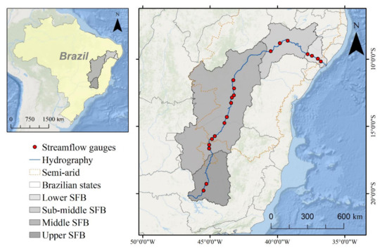
Figure 1.
The Sao Francisco River Basin (SFB) location and river gauges along the Sao Francisco River (SFR).
Irrigated agriculture is the most important economic activity in the SFB and is responsible for 86% of permitted surface water withdrawals [35]. However, the SFR also supplies water for ~16 million people in 521 municipalities [36] and has hydroelectric power plants that supply ~12% (10,708 Megawatt) of the installed generation capacity in Brazil [37]. The SFB accounts for 23% (~750 m3 s−1) of all the surface water abstraction permits in Brazil [35].
Although the average precipitation is 938 mm year−1 over the entire SFB [34], there is a large variation in precipitation within the SFB (Table 1). Due to its variability in precipitation regimes and biomes, the SFB is divided into four hydrographical regions: Upper, Middle, Sub-middle and Lower (Figure 1). The main characteristics (e.g., precipitation, climate classification and biome) of each hydrographical region are summarized in Table 1. The entire Sub-middle SFB, and most of the Lower and Middle SFB, are in the Brazilian Semiarid climate zone (Figure 1), which is considered the driest region in the country due to prolonged droughts. The spatial distribution of the precipitation, evapotranspiration and climate type are shown in Figure 2.

Table 1.
The main features of the hydrographical regions of the Sao Francisco River Basin (SFB).
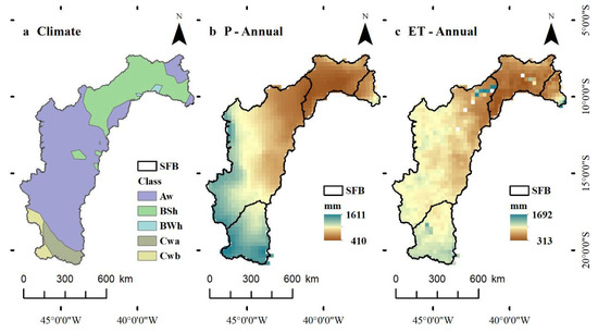
Figure 2.
The spatial distribution of: (a) the climate type according to Köppen’s classification; (b) annual mean precipitation (P); and (c) annual mean evapotranspiration (ET) over the Sao Francisco Basin (SFB).
2.2. Data Sources
2.2.1. Streamflow Data
We obtained daily streamflow records from 20 river gauges located in the SFR over the 1980–2015 period, which we averaged to the annual mean flow. The streamflow data were downloaded from the Brazilian Water Agency (ANA, Agencia Nacional de Aguas) website (http://www.snirh.gov.br/hidroweb/). The river gauges span the four hydrological regions, as follows: two gauges in the Upper SFB (40070000 and 40100000), 11 gauges in the Middle SFB (42210000, 43200000, 44200000, 44290000, 44500000, 45298000, 45480000, 46035000, 46105000, 46150000 and 46360000), three gauges in the Sub-middle SFB (48020000, 48290000 and 48590000) and four gauges in the Lower SFB (49330000, 49370000, 49660000 and 49705000).
2.2.2. Precipitation, Evapotranspiration and Water Storage Change Data
To evaluate potential drivers of streamflow changes in the SFB, we computed spatiotemporal trends in water fluxes (precipitation, P, evapotranspiration, ET, and total water storage, TWS). We used ground-based gridded rainfall to retrieve daily P data (from 1980 to 2015) with a 0.25° × 0.25° spatial resolution [42]. The gridded P data were obtained by interpolation technique using data from ~4000 rain gauges over Brazil i.e., [40] and have been widely used in regional studies [43,44,45,46].
Daily ET and potential ET (PET) was acquired from the Global Land Evaporation Amsterdam Model (GLEAM) dataset [47], with a 0.25° × 0.25° spatial resolution during the 1980–2015 period, which is available at https://www.gleam.eu/. GLEAM is dedicated to the estimation of terrestrial evaporation and root-zone soil moisture from satellite data [48]. Basically, GLEAM separately derives the different components of terrestrial evaporation, i.e., transpiration (from short and tall vegetation), bare soil evaporation, open-water evaporation, interception loss and sublimation on a daily basis [47]. GLEAM has been used to evaluate trends in ET at a global scale [49].
Additionally, we analyzed the monthly TWS anomaly with a 0.5° × 0.5° spatial resolution (from mid-2002 to 2015), measured by the Gravity Recovery and Climate Experiment (GRACE) satellite mission. GRACE measures temporal variations in the Earth’s gravity field, which can be used to estimate changes in TWS (i.e., surface water, snow, groundwater and soil moisture storage) [50]. GRACE-based monthly gravity products are officially processed and distributed by three processing centers: GeoforschungsZentrum Potsdam (GFZ), Jet Propulsion Laboratory (JPL) and Center for Space Research of the University of Texas at Austin (CSR). Traditionally, two approaches have been used to generate GRACE-based TWS solutions: spherical harmonics and mass concentration blocks (mascons) [51]. Here, we used the JPL Release 06 (RL06) mascons solution, which is available at https://grace.jpl.nasa.gov/data/get-data/jpl_global_mascons/.
Trends in the P, ET and TWS dataset were analyzed on an annual and seasonal basis. Seasons were defined as: DJF (December, January and February), MAM (March, April and May), JJA (June, July and August) and SON (September, October and November). We used the location of groundwater wells and information about irrigation withdrawals from the Brazilian Geological Survey (CPRM). Furthermore, we acquired land use and land cover information over the SFB from the MapBiomas Brazil Project. MapBiomas is a collaborative multi-institutional initiative to generate annual land cover and use maps at a 30-m resolution using automatic classification processes applied to satellite images [52]. The complete description of the MapBiomas Brazil Project and dataset can be accessed at http://mapbiomas.org.
2.3. Partitioning of Streamflow into Baseflow and Quickflow
We quantified trends in total streamflow (Qt), baseflow (Qb), representing slowly varying inputs to streamflow such as groundwater, and quickflow (Qq), representing quickly varying inputs to streamflow such as surface runoff. The baseflow regime was taken as being representative of the overall behavior of the groundwater contribution over the SFB. Digital filters have been widely used to estimate the contribution of groundwater to streamflow [44,53] and have been shown to be suitable in comparison to other approaches over large spatial scales [54,55,56]. We applied two digital filters to decompose Qt into Qb and Qq components at a daily resolution, and used the average value of Qb of the two filters. The Qt, Qb and Qq at a daily resolution were then aggregated at the annual timescale.
First, the one-parameter recursive digital filter [57] was applied to estimate Qb at a daily time step (i) as follows:
where is a single parameter of the filter. We assumed values of equal to 0.90, 0.925 and 0.95 to generate a realistic comparison to manual decomposition techniques [53,58].
We also applied a second, two-parameter digital filter by Eckhardt [59] at a daily time step, given by:
where is the maximum value of the baseflow index, and is the recession parameter [60]. Ref. [59] suggested predefined values for the parameter based on the hydrogeology of the watershed: = 0.80 for perennial streams with porous aquifers, = 0.50 for streams with porous aquifers, and = 0.25 for perennial streams with hard rock aquifers.
However, it is important to mention that these values may not be suitable for some other watersheds. Hence, we estimated both the and the parameter of the Eckhardt’s filter for each river gauge. First, the parameter was estimated using the matching strip method because it is a well-established and widely accepted method in hydrological science [61,62]. The overlapped streamflow recession segments were fitted against the time by means of the Maillet linear model [61,63] in order to obtain the recession constant, :
where is the streamflow on the first day of the recession,, and is the time on a daily scale.
The Maillet model reflects the linear relationship between the discharge and storage of groundwater, which is an assumption of the Eckhardt’s filter. The filter parameter a (Equation (3)) and the recession constant k (Equation (4)) are related by . We performed this procedure using the Master Recession Curve Parameterization tool (MRCPtool) in Matlab software [64]. Second, given the value of the a parameter, the was estimated following [65]. Although the estimation is challenging, we chose this approach in order to obtain a more realistic baseflow separation in the study area. The results of the a, k and parameters are shown in the Supplementary File.
To evaluate the role of the groundwater contribution to SFR, we chose the baseflow index () as the hydrological signature. The represents how extensive the groundwater contribution is to the streamflow [66]. It was calculated as a long-term ratio between and (Equation (5)) at a daily time step:
The was calculated for each gauge. High values (> 0.70) indicate that groundwater is the major contributor to streamflow [67]. Conversely, low values ( < 0.40) indicate that quickflow is predominant in terms of streamflow, attesting to a greater surface runoff [67].
2.4. Trend Analysis
Several studies have used a trend analysis to evaluate significant changes in streamflow [68], baseflow [30,69,70], and precipitation and/or evapotranspiration [71,72,73]. We applied the Mann–Kendall (MK) trend test (using a significance level, , of 0.05) to , and on an annual basis during 1980–2015. We also used the MK test to assess how the water fluxes were related to the trends in the total streamflow and its components. Moreover, we also used the MK test to assess the water fluxes (P, ET and TWS). A trend analysis of water fluxes was performed to evaluate their potential influence on trends.
The nonparametric MK test is widely used to describe increasing or decreasing trends in hydrological time series [74]. The MK test is advantageous because it does not require any assumptions regarding the distribution of the data and is not very sensitive to outliers [75]. Nonparametric trend tests usually require time series without autocorrelation [76]; that is, streamflow values must be independent of each other. With regard to river flow, serial correlation is usually present, especially on a daily and monthly basis [77]. Here, we assumed that temporal dependencies were only significant on a subannual scale [78].
The MK test indicates whether changes through time are significant or not. To estimate the trend magnitude, i.e., how much the variable changes by unit of time [79], we used the nonparametric Theil–Sen’s slope estimator [80,81].
3. Results
3.1. Streamflow and Baseflow Spatial Variation
Figure 3 shows the distribution of annual streamflow and baseflow for river gauges over the SFB. The median () and the upper and lower bounds of the interquartile range () of (25th 75th percentile) increased moving downstream from the Upper SFB (= 195 m3 s−1; 154 241 m3 s−1), to the Middle SFB (= 1907 m3 s−1; 1505 2378 m3 s−1), to the Sub-middle SFB ( = 1997 m3 s−1; 1745 2485 m3 s−1) (Figure 3). On the other hand, we observed a slight decrease in both the 25th percentile of and from the Sub-middle to the Lower SFB ( = 1920 m3 s−1; 1677 2535 m3 s−1).
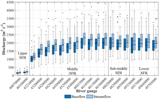
Figure 3.
Boxplot of the baseflow and streamflow of Sao Francisco River in the hydrographical regions (Upper, Middle, Sub-middle and Lower SFB) over the 1980–2015 period.
Similarly, the median within each hydrographical region () followed the behavior of . That is, increased from the Upper SFB ( = 173 m3 s−1; 129 203 m3 s−1), to the Middle SFB ( = 1732 m3 s−1; 1284 2092 m3 s−1), to the Sub-middle SFB ( = 1957 m3 s−1; 1565 2241 m3 s−1) (Figure 3). However, it is interesting that the increased from the Middle to the Sub-middle SFB was quite small. Furthermore, we found a slight decreased regime in both and the 25th percentile of from the Sub-middle to the Lower SFB ( = 1917 m3 s−1; 1493 2283 m3 s−1).
Baseflow, representing slowly varying water sources such as groundwater contributions, accounts for the large majority of in all hydrographical regions of the SFB. The BFI for all gauges exceeded 0.80, with relatively little difference in the BFI among gauges (Table 2). In general, the tended to increase from the Upper to Sub-middle SFB.
Table 2.
The annual trend magnitude for the streamflow (), baseflow () and quickflow () in the Sao Francisco Basin (SFB) according to the river gauge. Trends were assessed using the Mann–Kendall and Theil–Sen’s slope estimator at 0.05 of the significance level.
3.2. Trends in Streamflow, Baseflow and Quickflow
In general, we found a significant decreasing trend in , and (at = 0.05) over the SFB during 1980–2015 (Table 2). Trends in the two gauges located in the Upper SFB were not significant, while all other gauges had significant decreasing trends for all components of flow. Averaged over all gauges, in the SFB decreased at a rate of −24.15 m3 s−1 year−1 (1980–2015). The trend magnitude in varied from −12.87 to −32.52 m3 s−1 year−1 over the Middle SFB, from −25.35 to −29.74 m3 s−1 year−1 over the Sub−middle SFB, and from −24.71 to −29.79 m3 s−1 year−1 over the Lower SFB (Table 2). Overall, the trends observed in explain the large majority (86%) of the observed trends in , indicating that observed decreases in streamflow can be primarily attributed to changing baseflow conditions.
Similar to the trends in and , significant decreases in were found throughout the SFB (Table 2). The trend magnitude in ranged from −2.31 to −5.80 m3 s−1 year−1 in the Middle, from −4.37 to −5.32 m3 s−1 year−1 in the Sub−middle, and between −4.00 and −6.72 m3 s−1 year−1 in the Lower SFB. Overall, the trend magnitude in became more negative from the Middle to Sub−middle and Lower SFB. As a limitation, our spatial analysis approach did not explain the significant decreases in .
3.3. Trends in Precipitation, Evapotranspiration and Water Storage Changes
The annual and were not significant (at = 0.05) over most of the SFB during 1980–2015 (Figure 4c,d). Nevertheless, a significant decreasing trend in annual was observed in a few regions specifically over the western and northeastern part of the Middle SFB (Figure 4c), which is a region with widespread irrigation (Figure 4b). In addition, annual tended to decrease in a few regions over the central and western part of the Middle SFB, and in the Upper SFB (Figure 4d).
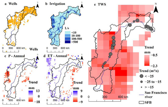
Figure 4.
(a) Location of the wells. (b) Irrigation demand over the Sao Francisco River. Annual trend magnitude: (c) precipitation (), (d) evapotranspiration (), and (e) terrestrial water storage change () and baseflow. Trends in baseflow along the Sao Francisco River are indicated by the grey circles. Trends were assessed using the Mann−Kendall and Theil–Sen’s slope estimator at 0.05 of the significance level. White color means a nonsignificant trend.
We also noted a significant negative trend in over almost all of the SFB, mainly over Middle SFB (Figure 4e) and the Sub−middle SFB (−1.4 ≤ ≤ −0.5 mm year−1; Figure 4e). On the other hand, a nonsignificant trend in was noted in the Lower SFB (Figure 4e). Particularly, one should note the spatial agreement between regions with decreasing and , decreasing , and increasing in the Middle SFB, which has the most irrigated agriculture in the region (Figure 4b–e). A strong trend magnitude in of −2.3 mm year−1 occurred in the Middle SFB around the SFR channel path near regions with large irrigation withdrawals over the west (Figure 4b,e).
The seasonal analysis revealed an overall nonsignificant trend in over the SFB (Figure 5a–d). The exception was a decrease in (−12 ≤ ≤ −1.0 mm year−1) over the western Middle SFB during the DJF season (Figure 5a). In addition, the also tended to increase ( = 9 mm year−1) strongly in a few regions over (and adjacent) to the Lower SFB during the JJA season (Figure 5c). Thus, in general, the seasonal results indicated that the decreases in annual P were primarily driven by reductions in the summer (DJF) precipitation.
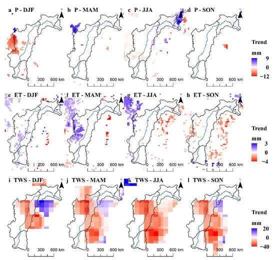
Figure 5.
Seasonal trend magnitude: (a–d) precipitation (), (e–h) evapotranspiration (), and (i–l) terrestrial water storage change (), and their magnitudes over the Sao Francisco Basin. DJF = December, January and February; MAM = March, April and May; JJA = June, July and August; and SON = September, October and November. Trends were assessed using the Mann−Kendall and Theil–Sen’s slope estimator at 0.05 of the significance level. White color means a nonsignificant trend.
We found a remarkable increasing trend in seasonal (3.0 ≤ ≤ 0.5 mm year−1) specifically in the heavily irrigated western and central parts of the Middle SFB during the MAM season (Figure 5f). The seasonal tended to increase by up to 1.0 mm year−1 during DJF (Figure 5e). Conversely, the results showed a slight decreasing trend in (−1.0 ≤ ≤ −3.0 mm year−1) during the SON season over the western Middle SFB. Additionally, in general, a nonsignificant trend in seasonal was observed in the Upper, Sub−middle and Lower SFB.
With regard to , we noted a negative trend in the western and eastern Middle SFB during all seasons (Figure 5i–l) where there were large irrigation demand and wells (Figure 4a,b). For instance, the strongest seasonal decreasing trend (−40 ≤ ≤ −20 mm year−1) showed a correspondence with the agricultural irrigation land over the western and central Middle SFB during MAM and JJA (Figure 5j,k). Furthermore, significantly increased from the JJA to SON and DJF seasons in the central-western and central-eastern parts of the Middle SFB. Conversely, there was a nonsignificant seasonal trend in the Upper, Sub−middle and Lower SFB.
4. Discussion
The partitioning of the total streamflow into a baseflow component reveals the major role of groundwater in sustaining the Sao Francisco River discharge. As a consequence, baseflow reductions are the primary driver of observed changes in the total streamflow. Our results show a strong decreasing trend in the annual baseflow and TWS over almost the entire SFB (Table 2 and Figure 4e), most prominently in the heavily irrigated Middle SFB (western and northeastern part). These results suggest that groundwater withdrawals for irrigation may be a driver that is likely responsible for decreased baseflow in the Middle SFB. This is supported by the spatial correspondence between irrigated agricultural land (Figure 4b), a decreasing annual (and seasonal) trend in (Figure 4e and Figure 5i–l), and a strong increasing trend in (Figure 5f,g). Unfortunately, data on direct surface water withdrawals from the SFR, which may also contribute to a decreasing trend in , are not available.
The close relation between increased and decreased over the irrigated area (i.e., the central-western part of the Middle SFB, which comprises the MATOPIBA region) can be related to deforestation for agricultural cropping. MATOPIBA is located mainly in the Bahia and Tocantins States, with irrigated holdings larger than 5000 ha and a water demand greater than 100 L s−1 [82]. Although this area also comprises rain-fed agriculture, irrigation is often required during dry periods. MATOPIBA experienced a significant expansion of the irrigated agriculture by center pivots from 13 to 1548 pivots during 1980–2015 [83]. Hence, given the expansion of agricultural land over the Middle SFB from 1985 to 2015 (Figure 6b), these lines of evidence combine to suggest that irrigated agricultural expansion induced an increase in groundwater withdrawals and, consequently, the increasing trend in during DJF and MAM. These withdrawals lead to a net increase in water export to the atmosphere (increased ), a decreasing , and ultimately a decrease in baseflow over the Middle SFB. This problem mirrors the challenges of diverse settings such as the United States, India and China, where marked increases in groundwater-fed irrigation in the last few decades have lowered groundwater levels and reduced streamflow [31,84].
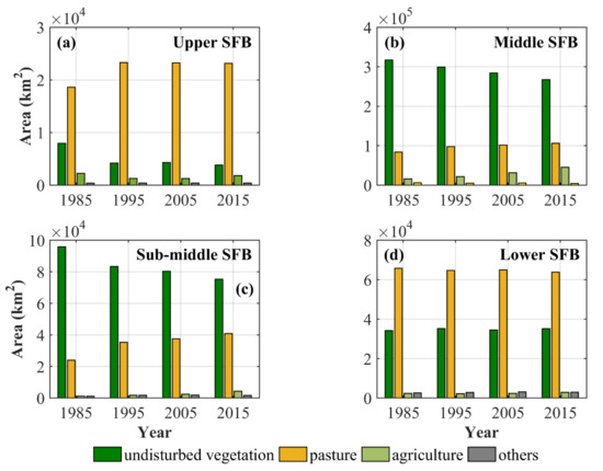
Figure 6.
Land use and cover area according to the hydrographical regions of the Sao Francisco River Basin (SFB) during 1985–2015: (a) Upper SFB, (b) Middle SFB, (c) Sub−middle SFB and (d) Lower SFB. Land use classes were acquired from MapBiomas 3.0 (http://mapbiomas.org/).
The decreased baseflow in the Middle SFB can be partly related to groundwater irrigation from the Urucuia Aquifer System (UAS). The UAS is a sedimentary aquifer that covers an area of 125,000 km2 and is an important source of water to the SFR, especially during dry seasons [72]. The UAS is located for the most part over the western Bahia State by the left bank of SFR and covers the MATOPIBA region. On average, the UAS discharged 792 m3 s−1 to the SFR in 1980; however, this contribution has decreased continuously to 390 m3 s−1 in 2015 [85]. In addition, a recent study showed that groundwater storage tended to decrease by 6.5 ± 2.6 mm year−1 (9.75 km3) in the UAS over the 2003–2014 period [72]. Therefore, given the importance of the UAS to SFR, it is reasonable to infer that groundwater decline in the UAS may have affected the SFR flow, particularly in the Middle SFB.
The Sub−middle SFB has been subjected to the expansion of irrigated agriculture (Figure 6), for example vineyards and mango orchards in the Juazeiro (Bahia State) and Petrolina municipalities (Pernambuco State) [86,87]. However, although a declined annual baseflow and TWS were found over the Sub-middle SFB (Figure 5e), significant trends in both annual and seasonal ET were not detected using GLEAM data. On the other hand, the declined annual TWS and nonsignificant trends in P may indicate that baseflow is affected by groundwater use. Moreover, the annual decreasing trend in occurred in the central-northern part of the Sub-middle SFB (Figure 5e) and near the SFB channel where irrigation from the SFR channel was present (Figure 4b). This indicates that in the Sub-middle SFB, it is likely that baseflow reduction is driven by combined surface and groundwater withdrawals. Furthermore, in future studies, trends in ET should be evaluated using different data sources.
5. Conclusions
Depletion streamflow has brought a major worldwide concern about water security, especially in (semi)arid regions. In Brazil, the Sao Francisco Basin (SFB) has experienced water-related problems because of decreased flow in the Sao Francisco River (SFR). The SFB is strategically important for the national food and energy production, with a huge irrigated area and a population of ~16 million. These multiple water demands make the SFR a socioeconomically important region, and balancing their needs poses a difficult task for decision makers.
Although previous studies have focused on the impacts of climate variability on decreasing SFR flow, none have addressed the possible influence of groundwater withdrawals. Here, we provide the first overview of long-term changes in relevant hydrological fluxes (i.e., precipitation, evapotranspiration, baseflow and water storage) in order to constrain potential drivers of the observed decrease in SFR flow over the SFB. We conducted a careful analysis by using different sources of data (satellite and ground-based) using a spatiotemporal approach that included 20 river gauges that measured data over the 1980−2015 period.
Our findings suggest that significant decreases in SFR flow are primarily due to reduced groundwater contributions to streamflow (i.e., baseflow) during the 1980–2015 period. The main results of TWS depletion and baseflow reduction indicate that groundwater pumping can decrease flow in the SFR. Therefore, groundwater withdrawals may be a likely driver of the observed negative trend in the SFR baseflow, especially in the most heavily irrigated Middle SFB region.
Because the Brazilian government has encouraged the expansion of irrigated agriculture to increase food production, in the future we expect further increased water demands from the SFB. Thus, we call for increased attention of groundwater use in the SFB in order to mitigate (or avoid) water-related problems such as those that have occurred in hotspots: the High Plains Aquifer (United States), part of the Central Valley Aquifer (United States), parts of Mexico (e.g., [32]), and the Ganges River Basins (India) (e.g., [30,32]). In this sense, surface−subsurface interactions should not be neglected in order to mitigate the impacts of groundwater overexploitation on river flow. This can be done, for instance, by adopting dynamical water use rights, e.g., [88].
As a limitation, groundwater storage changes were not isolated from the TWS signal. Moreover, future investigations are necessary to deeply identify the causes of decreased baseflow over the entire SFB, and the relative importance of climate and anthropic drivers in TWS changes. Furthermore, other studies should be done to predict possible future scenarios of streamflow depletion resulting from the expansion of irrigated agriculture.
Supplementary Materials
The following are available online at https://www.mdpi.com/2073-4441/13/1/2/s1, Figure S1: Master Recession Curve (MCR) using the matching strip method for each river gauge in the SFB. The cyan line indicates linear fit through Maillet model. The recession parameter, a, of Eckhardt’s filter is also presented. Figure S2: Maximum Baseflow Index (BFImax) parameter running the backwards moving filter for each river gauge in the SFB. Figure S3: Baseflow separation and Baseflow Index (BFI) values using Eckhardt’s digital filter for each river gauge in the SFB over the 1980–2015 period. Table S1: Summary of the results of baseflow separation.
Author Contributions
Conceptualization, N.K., D.B.B.R. and P.T.S.O.; Formal analysis, N.K., D.B.B.R., A.A.M.N., A.A., D.d.C.D.M., S.C.Z. and P.T.S.O.; Funding acquisition, P.T.S.O.; Investigation, M.C.L.; Methodology, M.C.L., N.K., D.B.B.R., A.A.M.N., A.A., D.d.C.D.M. and P.T.S.O.; Project administration, D.B.B.R. and P.T.S.O.; Supervision, P.T.S.O.; Writing—original draft, M.C.L.; Writing—review & editing, D.B.B.R., A.A.M.N., A.A., D.d.C.D.M., S.C.Z. and P.T.S.O. All authors have read and agreed to the published version of the manuscript.
Funding
This research was funded by the Ministry of Science, Technology, Innovation and Communication—MCTIC and National Council for Scientific and Technological Development—CNPq (grants 441289/2017−7, 306830/2017−5, and 409093/2018−1) and Coordenação de Aperfeiçoamento de Pessoal de Nível Superior–Brasil–CAPES (Finance Code 001 and Capes PrInt).
Conflicts of Interest
The authors declare no conflict of interest.
References
- WEF—World Economic Forum. The Global Risks Report 2019, 14th ed.; World Economic Forum: Cologny/Geneva, Switzerland, 2019; ISBN 978-1-944835-15-6. [Google Scholar]
- Cosgrove, W.J.; Loucks, D.P. Water management: Current and future challenges and research directions. Water Resour. Res. 2015, 51, 4823–4839. [Google Scholar] [CrossRef]
- UN—United Nations. The Millennium Development Goals Report; Way, C., Ed.; United Nations: New York, NY, USA, 2015; ISBN 978-92-1-101320-7. [Google Scholar]
- Liu, J.; Yang, H.; Gosling, S.N.; Kummu, M.; Flörke, M.; Pfister, S.; Hanasaki, N.; Wada, Y.; Zhang, X.; Zheng, C.; et al. Water scarcity assessments in the past, present, and future. Earth Futur. 2017, 5, 545–559. [Google Scholar]
- Van Loon, A.F.; Van Lanen, H.A.J. Making the distinction between water scarcity and drought using an observation-modeling framework. Water Resour. Res. 2013, 49, 1483–1502. [Google Scholar] [CrossRef]
- Kummu, M.; Guillaume, J.H.A.; De Moel, H.; Eisner, S.; Flörke, M.; Porkka, M.; Siebert, S.; Veldkamp, T.I.E.; Ward, P.J. The world’s road to water scarcity: Shortage and stress in the 20th century and pathways towards sustainability. Sci. Rep. 2016, 6, 1–16. [Google Scholar] [CrossRef]
- Wada, Y.; Van Beek, L.P.; Wanders, N.; Bierkens, M.F. Human water consumption intensifies hydrological drought worldwide. Environ. Res. Lett. 2013, 8, 34036. [Google Scholar] [CrossRef]
- Hoekstra, A.Y. Water scarcity challenges to business. Nat. Clim. Chang. 2014, 4, 318–320. [Google Scholar]
- Vörösmarty, C.J.; McIntyre, P.B.; Gessner, M.O.; Dudgeon, D.; Prusevich, A.; Green, P.; Glidden, S.; Bunn, S.E.; Sullivan, C.A.; Liermann, C.R.; et al. Global threats to human water security and river biodiversity. Nature 2010, 467, 555–561. [Google Scholar] [CrossRef]
- Veldkamp, T.I.E.; Wada, Y.; Aerts, J.C.J.H.; Döll, P.; Gosling, S.N.; Liu, J.; Masaki, Y.; Oki, T.; Ostberg, S.; Pokhrel, Y.; et al. Water scarcity hotspots travel downstream due to human interventions in the 20th and 21st century. Nat. Commun. 2017, 8, 1–12. [Google Scholar] [CrossRef]
- Döll, P.; Fiedler, K.; Zhang, J. Global-scale analysis of river flow alterations due to water withdrawals and reservoirs. Hydrol. Earth Syst. Sci. 2009, 13, 2413–2432. [Google Scholar] [CrossRef]
- Arnell, N.W.; Gosling, S.N. The impacts of climate change on river flow regimes at the global scale. J. Hydrol. 2013, 486, 351–364. [Google Scholar] [CrossRef]
- Döll, P.; Zhang, J. Impact of climate change on freshwater ecosystems: A global-scale analysis of ecologically relevant river flow alterations. Hydrol. Earth Syst. Sci. 2010, 14, 783–799. [Google Scholar] [CrossRef]
- Flörke, M.; Schneider, C.; McDonald, R.I. Water competition between cities and agriculture driven by climate change and urban growth. Nat. Sustain. 2018, 1, 51–58. [Google Scholar] [CrossRef]
- Gesualdo, G.C.; Oliveira, P.T.; Rodrigues, D.B.B.; Gupta, H.V. Assessing water security in the São Paulo metropolitan region under projected climate change. Hydrol. Earth Syst. Sci. 2019, 23, 4955–4968. [Google Scholar] [CrossRef]
- Gleeson, T.; VanderSteen, J.; Sophocleous, M.A.; Taniguchi, M.; Alley, W.M.; Allen, D.M.; Zhou, Y. Groundwater sustainability strategies. Nat. Geosci. 2010, 3, 378–379. [Google Scholar] [CrossRef]
- Castle, S.L.; Thomas, B.F.; Reager, J.T.; Rodell, M.; Swenson, S.C.; Famiglietti, J.S. Groundwater depletion during drought threatens future water security of the Colorado River Basin. Geophys. Res. Lett. 2014, 41, 5904–5911. [Google Scholar] [CrossRef]
- Döll, P.; Müller Schmied, H.; Schuh, C.; Portmann, F.T.; Eicker, A. Global-scale assessment of groundwater depletion and related groundwater abstractions: Combining hydrological modeling with information from well observations and GRACE satellites. Water Resour. Res. 2014, 50, 5698–5720. [Google Scholar] [CrossRef]
- Famiglietti, J.S. The global groundwater crisis. Nat. Clim. Chang. 2014, 4, 945–948. [Google Scholar] [CrossRef]
- Gleeson, T.; Wada, Y.; Bierkens, M.F.P.; Van Beek, L.P.H. Water balance of global aquifers revealed by groundwater footprint. Nature 2012, 488, 197–200. [Google Scholar] [CrossRef]
- Rodell, M.; Famiglietti, J.S.; Wiese, D.N.; Reager, J.T.; Beaudoing, H.K.; Landerer, F.W.; Lo, M.H. Emerging trends in global freshwater availability. Nature 2018, 557, 651–659. [Google Scholar] [CrossRef]
- Scanlon, B.R.; Faunt, C.C.; Longuevergne, L.; Reedy, R.C.; Alley, W.M.; McGuire, V.L.; McMahon, P.B. Groundwater depletion and sustainability of irrigation in the US High Plains and Central Valley. Proc. Natl. Acad. Sci. USA 2012, 109, 9320–9325. [Google Scholar] [CrossRef]
- Voss, K.A.; Famiglietti, J.S.; Lo, M.; de Linage, C.; Rodell, M.; Swenson, S.C. Groundwater depletion in the Middle East from GRACE with implications for transboundary water management in the Tigris-Euphrates-Western Iran region. Water Resour. Res. 2013, 49, 904–914. [Google Scholar] [CrossRef] [PubMed]
- Richey, A.S.; Thomas, B.F.; Lo, M.; Reager, J.T.; Famiglietti, J.S.; Voss, K.; Swenson, S.; Rodell, M. Quantifying renewable groundwater stress with GRACE. Water Resour. Res. 2015, 51, 5217–5238. [Google Scholar] [CrossRef] [PubMed]
- Lettenmaier, D.P.; Alsdorf, D.; Dozier, J.; Huffman, G.J.; Pan, M.; Wood, E.F. Inroads of remote sensing into hydrologic science during the WRR era. Water Resour. Res. 2015, 51, 7309–7342. [Google Scholar] [CrossRef]
- Gleeson, T.; Richter, B. How much groundwater can we pump and protect environmental flows through time? Presumptive standards for conjunctive management of aquifers and rivers. River Res. Appl. 2018, 34, 83–92. [Google Scholar] [CrossRef]
- Barlow, P.M.; Leake, S.A. Streamflow Depletion by Wells—Understanding and Managing the Effects of Groundwater Pumping on Streamflow; Geological Survey: Reston, VA, USA, 2012. [Google Scholar]
- Zipper, S.C.; Dallemagne, T.; Gleeson, T.; Boerman, T.C.; Hartmann, A. Groundwater Pumping Impacts on Real Stream Networks: Testing the Performance of Simple Management Tools. Water Resour. Res. 2018, 54, 5471–5486. [Google Scholar] [CrossRef]
- Zipper, S.C.; Gleeson, T.; Kerr, B.; Howard, J.K.; Rohde, M.M.; Carah, J.; Zimmerman, J. Rapid and Accurate Estimates of Streamflow Depletion Caused by Groundwater Pumping Using Analytical Depletion Functions. Water Resour. Res. 2019, 55, 5807–5829. [Google Scholar] [CrossRef]
- Mukherjee, A.; Bhanja, S.N.; Wada, Y. Groundwater depletion causing reduction of baseflow triggering Ganges river summer drying. Sci. Rep. 2018, 8, 1–9. [Google Scholar] [CrossRef]
- Scanlon, B.R.; Jolly, I.; Sophocleous, M.; Zhang, L. Global impacts of conversions from natural to agricultural ecosystems on water resources: Quantity versus quality. Water Resour. Res. 2007, 43. [Google Scholar] [CrossRef]
- De Graaf, I.E.M.; Gleeson, T.; van Beek, L.P.H.; Sutanudjaja, E.H.; Bierkens, M.F.P. Environmental flow limits to global groundwater pumping. Nature 2019, 574, 90–94. [Google Scholar] [CrossRef]
- OAS/GEF/ANA. São Francisco River Basin—Integrated Management of Land Based Activities in the São Francisco River Basin; Washington, DC, USA. 2005. Available online: https://www.oas.org/dsd/SAFUP/sf.HTM (accessed on 21 December 2020).
- ANA—Agência Nacional de Águas. Brazilian Water Resources Report—2017; Full Report; Agência Nacional de Águas: Brasília, Brazil, 2018. [Google Scholar]
- ANA—Agência Nacional de Águas. Conjuntura dos Recursos Hídricos no Brasil 2019: Informe Anual; Agência Nacional de Águas: Brasília, Brazil, 2019. [Google Scholar]
- CODEVASF—Companhia de Desenvolvimento dos Vales dSão Francisco e do Parnaíba. Plano Nascente São Francisco: Plano de Preservação e Recuperação de Nascentes da Bacia do rio São Francisco; de Oliveira Motta, E.J., Gonçalves, N.E.W., Eds.; Editora iABS: Brasília, Brazil, 2016; ISBN 978-85-64478-39-8. [Google Scholar]
- ANA—Agência Nacional de Águas Sala de Situação da Agência Nacional de Águas. Available online: https://www.ana.gov.br/sala-de-situacao/sao-francisco/sao-francisco-saiba-mais (accessed on 13 April 2020).
- ANA—Agência Nacional de Águas. Conjuntura dos Recursos Hídricos: Informe 2015; Agência Nacional de Águas: Brasília, Brazil, 2015. [Google Scholar]
- IBGE—Instituto Brasileiro de Geografia e Estatística Censo Demográfico. Available online: https://censo2010.ibge.gov.br/ (accessed on 9 June 2020).
- MMA—Ministério do Meio Ambiente. Caderno da Região Hidrográfica do São Francisco; Ministério do Meio Ambiente: Brasília, Brazil, 2006. [Google Scholar]
- CBHSF—Comitê da Bacia Hidrográfica do Rio São Francisco. Plano de Recursos Hídricos da Bacia Hidrográfica do Rio São Francisco 2016-2025; Comitê da Bacia Hidrográfica do Rio São Francisco: Alagoas, Brazil, 2020. [Google Scholar]
- Xavier, A.C.; King, C.W.; Scanlon, B.R. Daily gridded meteorological variables in Brazil (1980–2013). Int. J. Climatol. 2016, 36, 2644–2659. [Google Scholar] [CrossRef]
- Gadelha, A.N.; Coelho, V.H.R.; Xavier, A.C.; Barbosa, L.R.; Melo, D.C.D.; Xuan, Y.; Huffman, G.J.; Petersen, W.A.; das Almeida, C.N. Grid box-level evaluation of IMERG over Brazil at various space and time scales. Atmos. Res. 2019, 218, 231–244. [Google Scholar] [CrossRef]
- Gómez, D.; Melo, D.C.D.; Rodrigues, D.B.B.; Xavier, A.C.; Guido, R.C.; Wendland, E. Aquifer Responses to Rainfall through Spectral and Correlation Analysis. JAWRA J. Am. Water Resour. Assoc. 2018, 54, 1341–1354. [Google Scholar] [CrossRef]
- De Melo, D.C.D.; Scanlon, B.R.; Zhang, Z.; Wendland, E.; Yin, L. Reservoir storage and hydrologic responses to droughts in the Paraná River basin, south-eastern Brazil. Hydrol. Earth Syst. Sci. 2016, 20, 4673–4688. [Google Scholar] [CrossRef]
- De Melo, D.C.D.; Xavier, A.C.; Bianchi, T.; Oliveira, P.T.S.; Scanlon, B.R.; Lucas, M.C.; Wendland, E. Performance evaluation of rainfall estimates by TRMM Multi-satellite Precipitation Analysis 3B42V6 and V7 over Brazil. J. Geophys. Res. Atmos. 2015, 120, 9426–9436. [Google Scholar] [CrossRef]
- Miralles, D.G.; Holmes, T.R.H.; De Jeu, R.A.M.; Gash, J.H.; Meesters, A.G.C.A.; Dolman, A.J. Global land-surface evaporation estimated from satellite-based observations. Hydrol. Earth Syst. Sci. 2011, 15, 453–469. [Google Scholar] [CrossRef]
- Martens, B.; Miralles, D.G.; Lievens, H.; van der Schalie, R.; de Jeu, R.A.M.; Fernández-Prieto, D.; Beck, H.E.; Dorigo, W.A.; Verhoest, N.E.C. GLEAM v3: Satellite-based land evaporation and root-zone soil moisture. Geosci. Model Dev. 2017, 10, 1903–1925. [Google Scholar] [CrossRef]
- Miralles, D.G.; Van Den Berg, M.J.; Gash, J.H.; Parinussa, R.M.; De Jeu, R.A.M.; Beck, H.E.; Holmes, T.R.H.; Jiménez, C.; Verhoest, N.E.C.; Dorigo, W.A.; et al. El Niño-La Niña cycle and recent trends in continental evaporation. Nat. Clim. Chang. 2014, 4, 122–126. [Google Scholar] [CrossRef]
- Rodell, M.; Velicogna, I.; Famiglietti, J.S. Satellite-based estimates of groundwater depletion in India. Nature 2009, 460, 999–1002. [Google Scholar] [CrossRef]
- Watkins, M.M.; Wiese, D.N.; Yuan, D.-N.; Boening, C.; Landerer, F.W. Improved methods for observing Earth’s time variable mass distribution with GRACE using spherical cap mascons. J. Geophys. Res. Solid Earth 2015, 120, 2648–2671. [Google Scholar] [CrossRef]
- MAPBIOMAS Project MapBiomas—Collection 3.0 of Brazilian Land Cover & Use Map Series. Available online: https://mapbiomas.org/ (accessed on 9 June 2020).
- Nathan, R.J.; McMahon, T.A. Evaluation of automated techniques for base flow and recession analyses. Water Resour. Res. 1990, 26, 1465–1473. [Google Scholar] [CrossRef]
- Lott, D.A.; Stewart, M.T. Base flow separation: A comparison of analytical and mass balance methods. J. Hydrol. 2016, 535, 525–533. [Google Scholar] [CrossRef]
- Xie, J.; Liu, X.; Wang, K.; Yang, T.; Liang, K.; Liu, C. Evaluation of typical methods for baseflow separation in the contiguous United States. J. Hydrol. 2020, 583, 124628. [Google Scholar] [CrossRef]
- Zhang, J.; Zhang, Y.; Song, J.; Cheng, L. Evaluating relative merits of four baseflow separation methods in Eastern Australia. J. Hydrol. 2017, 549. [Google Scholar] [CrossRef]
- Lyne, L.D.; Hollick, M. Stochastic time-variable rainfall runoff modelling. In Proceedings of the Hydrology and Water Resources Symposium; Institution of Engineers Australia: Perth, Australia, 1979; pp. 89–92. [Google Scholar]
- Arnold, J.G.; Allen, P.M.; Muttiah, R.; Bernhardt, G. Automated Base Flow Separation and Recession Analysis Techniques. Ground Water 1995, 33, 1010–1018. [Google Scholar] [CrossRef]
- Eckhardt, K. How to construct recursive digital filters for baseflow separation. Hydrol. Process. 2005, 19, 507–515. [Google Scholar] [CrossRef]
- Eckhardt, K. A comparison of baseflow indices, which were calculated with seven different baseflow separation methods. J. Hydrol. 2008, 352, 168–173. [Google Scholar] [CrossRef]
- Tallaksen, L.M. A review of baseflow recession analysis. J. Hydrol. 1995, 165, 349–370. [Google Scholar] [CrossRef]
- Posavec, K.; Parlov, J.; Nakić, Z. Fully Automated Objective-Based Method for Master Recession Curve Separation. Groundwater 2010, 48, 598–603. [Google Scholar] [CrossRef]
- Maillet, E. Essai d’Hydraulique Souterraine et Fluviale: Librairie Scientifique; Hermann: Paris, France, 1905. [Google Scholar]
- Carlotto, T.; Chaffe, P.L.B. Master Recession Curve Parameterization Tool (MRCPtool): Different approaches to recession curve analysis. Comput. Geosci. 2019, 132, 1–8. [Google Scholar] [CrossRef]
- Collischonn, W.; Fan, F.M. Defining parameters for Eckhardt’s digital baseflow filter. Hydrol. Process. 2013, 27, 2614–2622. [Google Scholar] [CrossRef]
- Yoshida, T.; Troch, P.A. Coevolution of volcanic catchments in Japan. Hydrol. Earth Syst. Sci. 2016, 20, 1133–1150. [Google Scholar] [CrossRef]
- Sawicz, K.; Wagener, T.; Sivapalan, M.; Troch, P.A.; Carrillo, G. Catchment classification: Empirical analysis of hydrologic similarity based on catchment function in the eastern USA. Hydrol. Earth Syst. Sci. 2011, 15, 2895–2911. [Google Scholar] [CrossRef]
- Rice, J.S.; Emanuel, R.E.; Vose, J.M.; Nelson, S.A.C. Continental U.S. streamflow trends from 1940 to 2009 and their relationships with watershed spatial characteristics. Water Resour. Res. 2015, 51, 6262–6275. [Google Scholar] [CrossRef]
- Ficklin, D.L.; Robeson, S.M.; Knouft, J.H. Impacts of recent climate change on trends in baseflow and stormflow in United States watersheds. Geophys. Res. Lett. 2016, 43, 5079–5088. [Google Scholar] [CrossRef]
- Hellwig, J.; Stahl, K. An assessment of trends and potential future changes in groundwater-baseflow drought based on catchment response times. Hydrol. Earth Syst. Sci. 2018, 22, 6209–6224. [Google Scholar] [CrossRef]
- Young, D.; Zégre, N.; Edwards, P.; Fernandez, R. Assessing streamflow sensitivity of forested headwater catchments to disturbance and climate change in the central Appalachian Mountains region, USA. Sci. Total Environ. 2019, 694, 133382. [Google Scholar] [CrossRef]
- Gonçalves, R.D.; Stollberg, R.; Weiss, H.; Chang, H.K. Using GRACE to quantify the depletion of terrestrial water storage in Northeastern Brazil: The Urucuia Aquifer System. Sci. Total Environ. 2019, 135845. [Google Scholar] [CrossRef]
- Valipour, M.; Bateni, S.M.; Gholami Sefidkouhi, M.A.; Raeini-Sarjaz, M.; Singh, V.P. Complexity of Forces Driving Trend of Reference Evapotranspiration and Signals of Climate Change. Atmosphere 2020, 11, 1081. [Google Scholar] [CrossRef]
- Gao, T.; Wang, H. Trends in precipitation extremes over the Yellow River basin in North China: Changing properties and causes. Hydrol. Process. 2017, 31, 2412–2428. [Google Scholar] [CrossRef]
- Hamed, K.H. Trend detection in hydrologic data: The Mann-Kendall trend test under the scaling hypothesis. J. Hydrol. 2008, 349, 350–363. [Google Scholar] [CrossRef]
- Bürger, G. On trend detection. Hydrol. Process. 2017, 31, 4039–4042. [Google Scholar] [CrossRef]
- Dibike, Y.B.; Solomatine, D.P. River flow forecasting using artificial neural networks. Phys. Chem. Earth Part B Hydrol. Ocean. Atmos. 2001, 26, 1–7. [Google Scholar] [CrossRef]
- Sabzevari, A.A.; Zarenistanak, M.; Tabari, H.; Moghimi, S. Evaluation of precipitation and river discharge variations over southwestern Iran during recent decades. J. Earth Syst. Sci. 2015, 124, 335–352. [Google Scholar] [CrossRef]
- Drápela, K.; Drápelová, I. Application of Mann-Kendall Test and the Sen’s Slope Estimates for Trend Detection in Deposition data From Bílý Kříž (Beskydy Mts., the Czech Republic 1997–2010); Beskydy: Brno, Czech Republic, 2011. [Google Scholar]
- Sen, P.K. Estimates of the Regression Coefficient Based on Kendall’s Tau. J. Am. Stat. Assoc. 1968, 63, 1379–1389. [Google Scholar] [CrossRef]
- Theil, H. Rank-invariant Method of Linear and Polynomial Regression Analysis, 1-2; Confidence Regions for the Parameters of Linear Regression Equations in Two, Three and More Variables: (proceedings Knaw, _5_3(1950), Nr 3/4, Indagationes Mathematicae, _1_2(1950); Stichting Mathematisch Centrum, Statistische Afdeling: Amsterdam, The Netherlands, 1949. [Google Scholar]
- Oliveira PT, S.; Almagro, A.; Colman, C.B.; Kobayashi AN, A.; Rodrigues DB, B.; Neto, A.M. Nexus of water-food-energy-ecosystem services in the Brazilian Cerrado. In Water and Climate Modeling in Large Basins 5; Silva, R.C.V., Tucci, C.E.M., Scott, C.A., Eds.; ABRHidro: Porto Alegre, Brazil, 2019; pp. 7–30. [Google Scholar]
- Landau, E.C.; Guimarães, D.P.; de Sousa, D.L. Expansão Geográfica da Agricultura Irrigada por Pivôs Centrais na Região do Matopiba Entre 1985 e 2015, 1st ed.; Landau, E.C., Ed.; Embrapa Milho e Sorgo: Sete Lagoas, Brazil, 2016; ISBN 1679-0154. [Google Scholar]
- Kustu, M.D.; Fan, Y.; Robock, A. Large-scale water cycle perturbation due to irrigation pumping in the US High Plains: A synthesis of observed streamflow changes. J. Hydrol. 2010, 390, 222–244. [Google Scholar] [CrossRef]
- Gonçalves, R.D.; Engelbrecht, B.Z.; Chang, H.K. Evolução da contribuição do Sistema Aquífero Urucuia para o Rio São Francisco, Brasil. Águas Subterrâneas 2018, 32, 1–10. [Google Scholar] [CrossRef]
- Andrade, V.P.M.; da Silva, J.A.B.; de Sousa, J.S.C.; Oliveira, F.F.; Simões, W.L. Aspectos fisiológicos de videira submetida a manejos de irrigação e fertilização. Pesqui. Agropecu. Trop. 2017, 47, 390–398. [Google Scholar] [CrossRef][Green Version]
- Teixeira, A.H.d.C. Determining Regional Actual Evapotranspiration of Irrigated Crops and Natural Vegetation in the São Francisco River Basin (Brazil) Using Remote Sensing and Penman-Monteith Equation. Remote Sens. 2010, 2, 1287–1319. [Google Scholar] [CrossRef]
- Gómez, D.; Wendland, E.; Carvalho Diniz Melo, D. Empirical rainfall-based model for defining baseflow and dynamical water use rights. River Res. Appl. 2020, 36, 189–198. [Google Scholar] [CrossRef]


Publisher’s Note: MDPI stays neutral with regard to jurisdictional claims in published maps and institutional affiliations. |
© 2020 by the authors. Licensee MDPI, Basel, Switzerland. This article is an open access article distributed under the terms and conditions of the Creative Commons Attribution (CC BY) license (http://creativecommons.org/licenses/by/4.0/).